arXiv:1709.00298v1 [astro-ph.SR] 1 Sep 2017
Determining the metallicity of the solar envelope using
seismic inversion techniques
Ga¨el Buldgen
1
⋆
, S. J. A. J. Salmon
1
, A. Noels
1
, R. Scuflaire
1
, M. A. Dupret
1
,
and D. R. Reese
2
1STAR Institute, Universit´e de Li`ege, All´ee du Six Aoˆut 19C, B-4000 Li`ege, Belgium
2LESIA, Observatoire de Paris, PSL Research University, CNRS, Sorbonne Universit´e, UPMC Univ. Paris 06, Univ. Paris Diderot, Sorbonne Paris Cit´e, 5 place Jules Janssen, 92195 Meudon Cedex, France
Accepted XXX. Received YYY; in original form ZZZ
ABSTRACT
The solar metallicity issue is a long-lasting problem of astrophysics, impacting multi-ple fields and still subject to debate and uncertainties. While spectroscopy has mostly been used to determine the solar heavy elements abundance, helioseismologists at-tempted providing a seismic determination of the metallicity in the solar convective enveloppe. However, the puzzle remains since two independent groups prodived two radically different values for this crucial astrophysical parameter. We aim at provid-ing an independent seismic measurement of the solar metallicity in the convective enveloppe. Our main goal is to help provide new information to break the current stalemate amongst seismic determinations of the solar heavy element abundance. We start by presenting the kernels, the inversion technique and the target function of the inversion we have developed. We then test our approach in multiple hare-and-hounds exercises to assess its reliability and accuracy. We then apply our technique to solar data using calibrated solar models and determine an interval of seismic measurements for the solar metallicity. We show that our inversion can indeed be used to estimate the solar metallicity thanks to our hare-and-hounds exercises. However, we also show that further dependencies in the physical ingredients of solar models lead to a low accuracy. Nevertheless, using various physical ingredients for our solar models, we determine metallicity values between 0.008 and 0.014.
Key words: Sun: abundances – Sun: fundamental parameters – Sun: helioseismology – Sun: interior – Sun: oscillations
1 INTRODUCTION
Helioseismology, the study of solar pulsations, has led to a number of successes. Amongst these achievements, one finds the determination of the position of the base of the solar convective envelope (see Basu & Antia 1997, , and refer-ences therein.), the determination of the helium abundance in this region (Basu & Antia 1995) as well as the demonstra-tion of the necessity of microscopic diffusion to accurately reproduce the acoustic structure of the Sun (Antia & Basu 1994). Another important result of helioseismology was the determination of the solar rotation profile (Brown et al. 1989; Kosovichev et al. 1997; Schou et al. 1998). However, the agreement that existed between solar models and struc-tural inversions has been reduced since the publication of updated abundance tables by Asplund et al. (2005) which
⋆
E-mail: [email protected]
showed a significant decrease of the metallicity with respect to the value commonly used in the standard solar models in the 90s (Grevesse & Noels 1993;Grevesse & Sauval 1998, hereafter GN93 and GS98, respectively). These tables were further improved in Asplund et al. (2009) and have been at the center of what is now called the “solar metallicity problem”. In 2011,Caffau et al.(2011) published new abun-dance tables for which the metallicity was again re-increased. Attempts were also made to carry out seismic determina-tions of the solar metallicity, the first of which being that of Takata & Shibahashi(2001) that hinted at a possible metal-licity decrease 3 years before the release of the new spectro-scopic abundances, but could not conclude to the uncertain-ties in their inversion results. Antia & Basu (2006) deter-mined its value as 0.0172± 0.002 using an analysis of the dimensionless sound-speed gradient, denoted W(r). In con-trast,Vorontsov et al. (2014) determined that it should lie within 0.008 and 0.013 using a detailed analysis of the
adia-batic exponent of solar envelope models for various equations of state.
In this study, we present a new method to derive an estimate of the metallicity in the solar envelope using the SOLA inversion technique (Pijpers & Thompson 1994) and the classical linear integral relations between frequency dif-ferences and structural corrections developped for metallic-ity kernels. In Sect.2, we present the structural kernels used and the target function of our metallicity estimate. We also present the possible causes of uncertainties in this method. In Sect.3, we test our methodology in hare-and-hounds exer-cises and quantify the various contributions to the inversion errors. In Sect.4, we compute inversions of the solar metal-licity for various trade-off parameters and reference models using different equations of state, we then discuss the relia-bility of our results and how further tests could complement and improve our study.
2 METHODOLOGY
To carry out our structural inversions, we use the linear in-tegral relations obtained from the variational developments of the pulsation equations. The classical formulation of these relations is δνn,ℓ νn,ℓ = ∫ 1 0 Kn,ℓ ρ,c2 δ ρ ρ dx+ ∫ 1 0 Kn,ℓ c2,ρ δc2 c2 dx, (1)
which is used to carry out inversions of the solar sound speed profile. In this expression the notation δ denotes difference according to the following convention
δx x = x obs− xr e f x r e f , (2)
where x can be an individual frequency of harmonic degree ℓand radial order n or a structural variable such as the den-sity, ρ, or the squared adiabatic sound speed, c2=ΓP
1ρ, with
P the pressure and Γ1 = (dln P
dln ρ)S, the adiabatic exponent,
where S is the entropy. The differences between structural variables are taken at fixed fractional radius r/R with R the total radius and r the radial position. The Kn,l functions are the structural kernels associated with the thermodynamical variables found in the variational expression. These func-tions only depend on equilibrium quantities and the eigen-functions of the so-called reference model of the inversion.
Using appropriate techniques (seeBuldgen et al. 2017), one can derive structural kernels for a large number of vari-ables. Amongst them, one finds the kernels related to the convective parameter, A, defined as
A=dln ρ dln r − 1 Γ1 dln P dln r, (3)
presented inElliott (1996) as part of the(A, Γ1) structural
pair. It was initially used to test the equation of state. In this paper, we use the kernels of the(A,Y, Z) triplet presented in Buldgen et al. (2017), where Y is the helium mass fraction and Z the metallicity. We illustrate these kernels in figure 1. The first interesting point to notice is that the kernels associated with A have a very small amplitude compared to those of Y and Z. In addition, A has the convenient property of being 0 in the adiabatic region of the convective envelope. Similarly toElliott(1996) who considered the(A, Γ1) kernels
for carrying inversions of the Γ1profile in the Sun, the kernels
we suggest in the present study can be used to efficiently carry out seismic inversions of both Y and Z in convective regions. The variational relation we use to carry out our inversion hence reads as
δνn,ℓ νn,ℓ = ∫ 1 0 Kn,ℓ A,Y, Zδ Adx+ ∫ 1 0 Kn,ℓ Y, A, ZδY dx+ ∫ 1 0 Kn,ℓ Z,Y, AδZ dx, (4) with x the fractional radius.
Although this study focusses on determinations of Z, we also carried out inversions of the helium abundance and found them to be in agreement with the classical helioseismic result of 0.2485± 0.0035, yet, less precise. As a comparison, Vorontsov et al.(2014) found that the helium mass fraction in the solar envelope was betweeen 0.24 and 0.255, which is also in agreement with the interval of[0.242 0.255] we find. The main uncertainty in our determination is related to the physical ingredients in the models, leading to differences in Γ1. Indeed, one uses the relation
δΓ1 Γ1 = ( ∂ ln Γ1 ∂ ln P)ρ,Y, Z δP P + ( ∂ ln Γ1 ∂ ln ρ)P,Y, Z δ ρ ρ + ( ∂ ln Γ1 ∂Y )P,ρ, Z δY + (∂ ln Γ1 ∂ Z )P,ρ,Y δZ (5)
to obtain perturbations of Y and Z in the variational ex-pression. The main weakness in this approach is that the state derivatives of Γ1 can vary not only with the equation
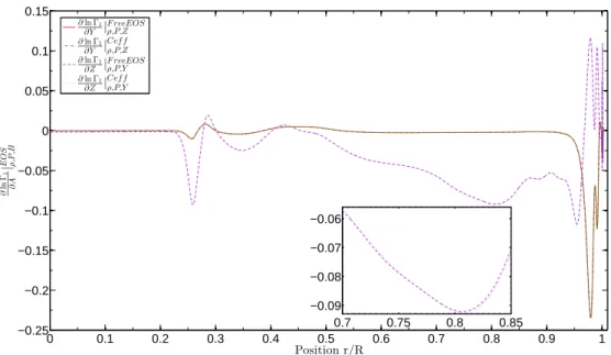
of state but also with the calibration. Indeed, the calibration process will lead to slight differences in the acoustic struc-ture when various physical ingredients (such as the opacity tables or the heavy elements abundance) are used. To as-sess this dependency, we use various physical ingredients in our hare-and-hounds exercises and our solar reference models used to determine the solar metallicity. A first il-lustration can be made, by comparing these derivatives for both the CEFF (Christensen-Dalsgaard & Daeppen 1992) and FreeEOS1(Irwin 2012) equations of state in a standard solar model. Both derivatives with respect to Y and Z are plotted in figure2and illustrate that the general behaviour of both curves is extremely similar. However, differences of nearly 0.001 can be seen in some regions and this of course means that, at the level of precision demanded, the choice of the equation of state will have an impact on the result. This is illustrated by the subplot of figure2, where we take a closer look at the differences between the state derivatives with respect to Z.
We define the target function of our indicator as follows, δZ = ∫ 1 0(1 − x)2exp−800(x−0.79) 2 δZ dx ∫01(1 − x)2exp−800(x−0.79) 2 dx = ∫ 1 0 TZδZ dx, (6)
which of course implies δZ = δZ in the envelope up to an excellent accuracy, firstly because the chemical abundances are constant in the fully mixed convective zone of the Sun and secondly, the weight function of the indicator is virtually 0outside of a small interval (in normalised radius) within the envelope. The location of the Gaussian has been chosen such that it is not close to the helium ionization zone, which
0 0.2 0.4 0.6 0.8 1 −0.2 −0.15 −0.1 −0.05 0 0.05 0.1 0.15 Position r/R K n ,l A ,Y K20,1 A,Y KA,Y30,0 KA,Y20,0 KA,Y25,2 0 0.2 0.4 0.6 0.8 1 −3 −2 −1 0 1 Position r/R K n ,l Y ,A KY,A20,1 KY,A30,0 KY,A20,0 KY,A25,2 0 0.1 0.2 0.3 0.4 0.5 0.6 0.7 0.8 0.9 1 −2 −1 0 1 2 3 Position r/R K n ,l Z ,A ,Y KZ,A,Y20,0 KZ,A,Y30,0 KZ,A,Y20,1 KZ,A,Y25,2
Figure 1.Kernels of the (A, Y, Z) triplet for various oscillation modes (Upper left panel, A Kernels) (Upper right panel, Y kernels) (Lower panel, Z kernels)
0 0.1 0.2 0.3 0.4 0.5 0.6 0.7 0.8 0.9 1 −0.25 −0.2 −0.15 −0.1 −0.05 0 0.05 0.1 0.15 Position r/R ∂ ln Γ1 ∂ A | E O S ρ ,P ,B ∂ln Γ1 ∂Y | F reeEOS ρ,P,Z ∂ln Γ1 ∂Y | Cef f ρ,P,Z ∂ln Γ1 ∂Z | F reeEOS ρ,P,Y ∂ln Γ1 ∂Z | Cef f ρ,P,Y 0.7 0.75 0.8 0.85 −0.09 −0.08 −0.07 −0.06
Figure 2.(Green and red curves) State derivatives of the natural logarithm of Γ1with respect to Y for the FreeEOS and CEFF equations of state. (Magenta and blue curves) State derivatives of the natural logarithm of Γ1with respect to Z for the FreeEOS and CEFF equations of state.
would imply a very strong correlation with the helium cross-term. The Gaussian width is also small enough so that there is no intensity in the radiative zone, which is not fully mixed. Looking at Figs. 1 and 2, one can also see that this region is characterised by a rather large intensity in the Γ1
derivatives with respect to Z, hence its associated kernels still having a non-negligible intensity around 0.8 while the helium kernels are nearly 0 at those depths.
For this indicator, the cost function of the SOLA inver-sion is written as,
JZ= ∫ 1 0 [KAvg− TZ] 2dx + β ∫01K2 Cross,Ydx+ β2∫ 1 0 K2 Cross, Adx + tan(θ)∑N i (c iσi)2+ λ [1 − ∫ 1 0 KAvgdx], (7)
where KAvg, KCross, Aand KCross,Y are the so-called averaging
and cross-term kernels (Pijpers & Thompson 1994). The av-eraging kernel is responsible for the matching of the target function of the inversion (thus the accuracy of the method). Meanwhile, the cross-term kernels are contributions for the additional variables found in Eq.4and which cannot be com-pletely annihilated. For this particular inversion, two cross-terms have to be taken into account since we work with a triplet of variables instead of a pair. This means that the trade-off problem (Backus & Gilbert 1967) has to be anal-ysed in depth and particular care has to be taken to check for possible compensation of the various error contributions in certain regions of the parameter space. The trade-off prob-lem is assessed in the classical way, using the parameter θ to avoid a large contribution from the observational errors and the parameters β and β2 to reduce each cross-term
contri-bution. The variable λ is no free parameter, but a Lagrange multiplier associated with the unimodularity constraint.
The trade-off problem, and thus the quality of the in-version, is analysed by looking separately at the amplitudes of the terms associated with the averaging and cross-term kernels in Eq.7. These terms are denoted
∣∣Kavg∣∣2= ∫ 1 0 [KAvg− TZ] 2 dx, (8) ∣∣KCr oss,Y∣∣2= ∫ 1 0 K2 Cross,Ydx, (9) ∣∣KCr oss, A∣∣2= ∫ 1 0 K2 Cross, Adx. (10)
However, these contributions do not contain all the infor-mation about the inversion technique. It is also useful to analyse separately each term of the inverted correction in hare-and-hounds exercises, to detect potential compensation effects. Therefore, we also analyse each error source of the inversion separately, using the definitions of Buldgen et al. (2015), which for this specific case are
ǫAVG= ∫ 1 0 [KAvg− TZ] δZdx, (11) ǫCross,Y= ∫ 1 0 KCross,YδY dx, (12) ǫCross, A= ∫ 1 0 K Cross,Aδ Adx, (13)
ǫRes= ZT ar− ZRe f − δZI nv− ǫAVG− ǫCross,Y− ǫCross, A,
(14) with ZT ar the metallicity of the target, which is known
in a hare-and-hounds exercises, ZRe f the metallicity of the
hound, δZI nv the inverted correction found using the
inver-sion. The residual error, ǫRes, which is obtained once all the
other errors have been subtracted from the inversion results, encompasses all aspects that are not properly treated by the inversion. These include, in the hare-and-hounds exercises, the potential inadequacy of the surface effect corrections or the non-linear aspects stemming from the non-verification of the linear equations4or the assumptions on the equation of state made through Eq.5.
3 HARE-AND-HOUNDS EXERCISES
Before carrying out the inversion on the actual solar seismic data, we carried out haand-hounds exercises to test the re-liability of the metallicity determination. The stellar models used in the exercises were computed using the Li`ege stellar evolution code (CLES,Scuflaire et al. (2008a)). Their fre-quencies and eigenfunctions were computed using the Li`ege adiabatic oscillation code (LOSC,Scuflaire et al.(2008b)). The inversions were computed using a customised version of the InversionKit software (Reese et al. 2012).
3.1 Methodology and results
We used a calibrated standard solar model built with the past solar GN93 (Grevesse & Noels 1993) abundances (high metallicity, Z) and the latest version of the Opal equation of state (Rogers & Nayfonov 2002) as our hare. Further-more, we used the latest OPLIB opacities (Colgan et al. 2016) supplemented at low temperature by the opacities of Ferguson et al.(2005) and the effects of conductivity from Potekhin et al.(1999) andCassisi et al.(2007). The nuclear reaction rates implemented were those from the NACRE project (Angulo et al. 1999), supplemented by the updated reaction rate fromFormicola et al. (2004) and we used the classical, local mixing-length theory (B¨ohm-Vitense 1958) to describe convective motions. The hounds were fitted to the hare to ensure that they had exactly the same radii and similar luminosities. They were computed with the AGSS09 abundances and either the CEFF or the FreeEOS equation of state. There are two reasons justifying the fact that we did not use the Opal equation of state in our reference mod-els. Firstly, this allows us to test for the biases stemming from the equation of state in our inversions. Secondly, the Opal equation of state, being defined on a grid with finite resolution, is not well suited to compute the Γ1 derivatives
numerically with high accuracy. The CEFF and FreeEOS equations of state, being defined with analytical relations, do not suffer from this problem and were thus favoured.
We summarise the properties of the hare and the hounds in table1. As can be seen, some of these reference models differ significantly from the target. These differences result from the way the hounds were generated, which was not a classical solar calibration as is usually done for the Sun. All hounds reproduce accurately the radius of target 1, a given value of helium abundance in the convective envelope and the position of its base within a less constraining ac-curacy. We did not limit the values of helium abundance and position of the base of the convective envelope to those of target 1 to assess the effects of those constraints on the
cross-term contributions. To further assess the uncertain-ties, additional changes were induced in Ref 1, 2 and 3 by not including microscopic diffusion of the heavy elements. The changes in the position of the base of the convective envelope for the various hounds were induced by changing the value of an undershoot parameter within values up to 0.2of the local pressure scale height before recalibrating the hounds. As can be seen from the luminosity and age values in table 1, this calibration method can lead to quite large differences between the models, hence sometimes implying larger differences in acoustic structure between the hare and the hounds than in a classical solar calibration approach.
We used the radius, the helium abundance in the con-vective envelope and the position of its base as constraints for the fit of the hounds to the hare. Once a satisfying fit was obtained, we changed an undershoot parameter and the diffusion velocities, while still fitting the radius, to be able to analyze the behaviour of the inversion when facing changes in A and Y . Consequently, some non-linearities could be ob-served for a few of these perturbed models and could help us understand the cases were the inversion was not so stable. To be as close to reality as possible, we used the exact same set of low ℓ oscillation modes observed for the Sun as pre-sented inBasu et al.(2009), namely 2189 oscillation modes with ℓ from 0 up to 250, and used the same uncertainties on the frequencies as those of the actual solar modes. We tested a total of 17 hounds and analysed whether the inversion was efficient in determining the metallicity of the hare. Due to the large differences between the hitherto seismically deter-mined values of the solar metallicity, we wanted to assess whether our method would be able to distinguish between several solutions.
The results of these inversions are given in table2and illustrated in figure3. For all the cases illustrated here, the inversion could determine an estimate of the metallicity in the convective envelope. However, one can see that for ref-erence models (hounds) 2, 10, 11 and 13, these estimates are not so accurate. Globally, a spread of around 4× 10⁻³is found for the inversion results. This spread is due to multi-ple sources: e.g., for models 10, 11 and 13, the equation of state was the CEFF equation of state, which leads to much larger differences in Γ1 with the Opal05 equation of state
than does the FreeEOS equation of state. Besides the differ-ences from the equation of state, intrinsic differdiffer-ences in Γ1
due to differences in stratification of the model, can have a strong impact on the accuracy of the method. It is important to bear in mind that the variables Y and Z are not directly seismically constrained but are obtained via an equation of state which is furthermore linearised using to Eq.5. Conse-quently, errors in the derivatives of Γ1can quickly arise and
reduce the accuracy of the results. Moreover, hounds having a poor representation of the stratification of the hare model will also have rather large A differences and thus intrinsically larger cross-term contributions. In Sect.3.2, we further in-vestigates this point and discuss the determination of the trade-off parameters and what they can teach us about the characteristics of our approach.
3.2 Analysis of the stability of the inversion technique
3.2.1 Quality of the kernel fits
We have seen in Sect.3.1that an indication of the metallicity of the Sun can be provided by seismology. However, inversion techniques can sometimes provide accurate results because of compensation of their errors. Therefore, their reliability and stability should be properly assessed.
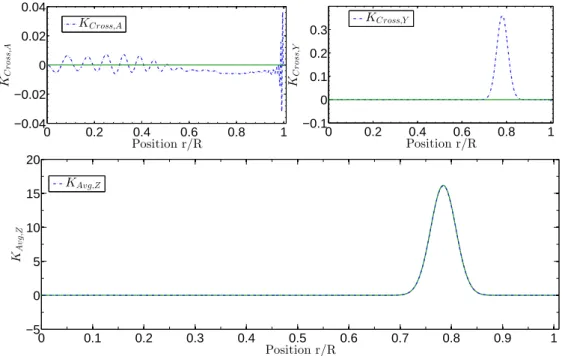
We propose to first assess the quality of the kernel fits by looking at the amplitude of the first three terms of Eq. 7, in the last columns of table 2. To give a better idea of what these represent, we illustrate in figure4the fit of the averaging kernel and the cross-term kernels for the inver-sion of Ref 3. From a first visual inspection, the fit of the averaging kernel seems good and the contribution from the cross-term associated with A seems close to 0. By inspecting the helium cross-term kernel, we can see a strong correlation with the averaging kernel. However, the height of this peak is around 45 times smaller than the height of the averag-ing kernel. This means that the helium contribution should be kept small, as can be seen in figure 5. This difference in amplitude is a consequence of the choice of the position for the peak in the target function. Had we chosen a target much closer to the helium ionization zones, then the corre-lation with the helium kernels would have been much more problematic.
To analyse whether compensation is present in the in-version, we plot in figure5the real error contributions for all hounds. The kernel fits are informative of the quality of the inversion. However plotting the real error contributions can indicate whether what appears visually as a satisfactory fit is actually the reason for the accuracy of the result.
3.2.2 Analysis of the parameter space
The main difficulty of carrying out the inversion is to find a given set of parameters for which the real errors of the in-version, here defined as the ǫiin Eqs.11to14, are small and
do not present compensation effects, and where the squared norm of the differences between the averaging and cross-term kernels, defined in Eqs. 8 to 9, and their respective targets have reduced amplitudes. Depending on the quality of the reference model or the dataset, the trade-off prob-lem will be different and multiple sets of parameters can be found. Therefore, to further understand the reliability of the inversion and its parameter dependency, we did for Ref 3 a brief scan of the parameter space, which is illustrated in fig-ure 6. Firstly, we note from the lowest left panel in figure 6, illustrating the differences between the inverted Z value and the target value of Z, that the changes in the parame-ter do not induce a large deviation of the inversion results from the value found with the optimal set of parameters. However, other inversions in our hare-and-hounds exercises were not as stable, mainly due to an increase of the residual error or to the cross-term contribution associated with the convective parameter. For this scan, we fixed a value of β2to
1.0and varied θ from 10−4to 10−9and β from 10−2to 101.5 (see eq.7). A first observation that can be made is that the variations of all quantities are regular with the parameters. Sudden and steep variations in the accuracy of the solution
Table 1.Characteristics of the models used in the hare-and-hounds exercises
Mass(M⊙) Age(Gy) Radius(R⊙) L (L⊙) YC Z ZC Z (Rr)C Z EOS
Target 1 1.0 4.5794 1.0 0.9997 0.2397 0.01818 0.07087 Opal05 Ref 1 1.0 4.8073 1.0 0.9564 0.2307 0.01513 0.07087 FreeEOS Ref 2 1.0 4.8038 1.0 0.9558 0.2294 0.01513 0.7125 FreeEOS Ref 3 1.0 4.5097 1.0 0.9740 0.2342 0.01513 0.716 FreeEOS Ref 4 1.0 4.2502 1.0 0.9933 0.2421 0.01513 0.7068 FreeEOS Ref 5 1.0 4.4130 1.0 1.0107 0.2455 0.01373 0.7161 FreeEOS Ref 6 1.0 5.0004 1.0 0.9749 0.2301 0.01375 0.7087 FreeEOS Ref 7 1.0 4.8743 1.0 0.9817 0.2300 0.01373 0.7171 FreeEOS Ref 8 1.0 4.4081 1.0 1.0100 0.2419 0.01381 0.7066 FreeEOS Ref 9 1.0 4.5285 1.0 1.0035 0.2381 0.01369 0.7160 FreeEOS Ref 10 1.0 5.3522 1.0 0.9695 0.2285 0.01358 0.7090 CEFF Ref 11 1.0 5.2909 1.0 0.9731 0.2282 0.01349 0.7150 CEFF Ref 12 1.0 5.2253 1.0 0.9761 0.2283 0.01345 0.7170 CEFF Ref 13 1.0 4.7455 1.0 1.0046 0.2402 0.01373 0.7055 CEFF Ref 14 1.0 4.8635 1.0 0.9982 0.2364 0.01361 0.7160 FreeEOS Ref 15 1.0 4.7433 1.0 1.0054 0.2283 0.01355 0.7236 FreeEOS Ref 16 1.0 4.5651 1.0 1.0155 0.2435 0.01376 0.7075 FreeEOS Ref 17 1.0 4.5790 1.0 0.9993 0.2435 0.01344 0.7120 FreeEOS Target 2 1.0 4.5787 1.0 1.0002 0.2386 0.01820 0.7080 FreeEOS
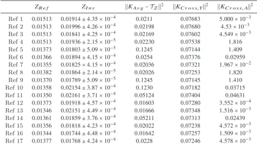
Table 2.Inversion results for the hare-and-hounds exercises.
ZR e f ZI n v ∣∣KAv g− TZ∣∣2 ∣∣KC r o s s,Y∣∣2 ∣∣KC r o s s,A∣∣2 Ref 1 0.01513 0.01914± 4.35 × 10⁻⁴ 0.0211 0.07683 5.000× 10⁻³ Ref 2 0.01513 0.01996± 4.26 × 10⁻⁴ 0.02198 0.07680 4.53× 10⁻³ Ref 3 0.01513 0.01841± 4.25 × 10⁻⁴ 0.02169 0.07602 4.549× 10⁻³ Ref 4 0.01513 0.01936± 2.15 × 10⁻⁵ 0.02230 0.07538 1.816 Ref 5 0.01373 0.01803± 5.09 × 10⁻⁵ 0.1245 0.07144 1.409 Ref 6 0.01366 0.01894± 4.15 × 10⁻⁴ 0.0254 0.07376 0.02959 Ref 7 0.01355 0.01825× 4.15 × 10−4 0.02036 0.07321 1.967× 10⁻² Ref 8 0.01382 0.01864± 2.14 × 10⁻⁵ 0.02026 0.07253 1.820 Ref 9 0.01370 0.01789± 5.09 × 10⁻⁵ 0.1245 0.07145 1.410 Ref 10 0.01358 0.02154± 3.87 × 10⁻⁴ 0.1230 0.07182 0.03715 Ref 11 0.01350 0.02161± 3.71 × 10⁻⁴ 0.05124 0.07404 0.04631 Ref 12 0.01373 0.01918± 4.57 × 10⁻⁴ 0.01603 0.07280 3.552× 10⁻⁴ Ref 13 0.01346 0.02151± 4.49 × 10⁻⁴ 0.01666 0.07348 1.516× 10⁻³ Ref 14 0.01361 0.01859± 3.76 × 10⁻⁴ 0.05211 0.07313 0.02439 Ref 15 0.01356 0.01818± 4.23 × 10⁻⁴ 0.02022 0.07238 4.572× 10⁻³ Ref 16 0.01344 0.01744± 4.48 × 10⁻⁴ 0.01642 0.07257 1.509× 10⁻³ Ref 17 0.01377 0.01768± 4.24 × 10⁻⁴ 0.0228 0.07246 4.578× 10⁻³
and the real error contributions would indicate that the in-version is not sufficiently regularised. In such cases, one has no real control on the trade-off problem and thus no means of ensuring a correct result.
In figure6, we can see that for a fixed value of β2 the
optimum is found for a low θ and a low β. However, the low β value has to be considered carefully when the helium abun-dance differences are larger. For this particular test between Ref 3 and Target 1, the differences is of the order of 0.005, thus intrinsically quite small, which naturally reduces the value of ǫCr oss,Y. In addition to the helium cross-term
con-tribution, the amplitude of the error bars could be strongly increased by the reduction of the θ parameter. In this par-ticular case, the lower plot of figure6shows that the error bars remained quite small for the whole scan but this will not necessarily be the case for other inversions.
Overall, we can see from the lower plot of figure6that
the inversion is very stable, since the errors remain of the order of 10−4, with the exception of the residual error that can reach is this case the order of 10−3for a particular region of the parameter set. This region is related to high values of β and β2 (which is fixed) and a range of low θ values of
around 10−8 and 10−9. This is a consequence of the regu-larising nature of the θ parameter, which is used to adjust the trade-off between precision and accuracy of the method. In this particular case, the instability of the inversion is a consequence of the very low weight given to the damping of the error bars, and thus the precision of the method. A similar behaviour can also be observed in solar inversions of full structural profiles, were the observational error bars remain small, but the profile already shows an unphysical oscillatory behaviour.
0
1
2
3
4
5
6
7
8
9 10 11 12 13 14 15 16 17 18
0.013
0.014
0.015
0.016
0.017
0.018
0.019
0.02
0.021
0.022
Model Number
Z
Reference models
Inverted results
Target value
Figure 3.Inversion results for the hare-and-hounds exercises between the 17 reference models and the target model of table1.
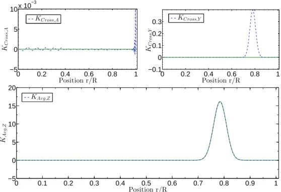
0 0.2 0.4 0.6 0.8 1 −0.04 −0.02 0 0.02 0.04 Position r/R KC r o ss ,A KCross,A 0 0.2 0.4 0.6 0.8 1 −0.1 0 0.1 0.2 0.3 Position r/R KC r o ss ,Y KCross,Y 0 0.1 0.2 0.3 0.4 0.5 0.6 0.7 0.8 0.9 1 −5 0 5 10 15 20 Position r/R KA v g ,Z KAvg,Z
Figure 4.(Upper-left panel) Cross-term associated with A in blue and the target function (being 0 here) in green. (Upper-right panel) Cross-term associated with Y in blue and the target function (being 0) in green. (Lower panel) Averaging kernel of the inversion in blue and the respective target function in green.
Our hare-and-hound exercises allowed us to define various parameter values for which the inversion was stable, depend-ing on the reference model quality. In most cases, the value of β, the free parameter associated with the helium contri-bution, was set between approximately 0.1 and 10, as can be seen in table 3, depending on the intrinsic difference in helium content between the target and the reference model. Indeed, if the helium abundance value is naturally close to
that of the target, it is unnecessary to strongly damp the he-lium cross-term and penalise the elimination of the convec-tive parameter cross-term. Actually, it should be noted that βand β2are correlated. As damping the helium cross-term is
done by reducing the amplitude of the inversion coefficients, it can sometimes have a similar effect on the convective pa-rameter cross-term.
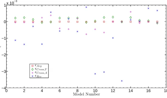
contri-0 2 4 6 8 10 12 14 16 18 −4 −3 −2 −1 0 1x 10 −3 Model Number ǫ ǫAvg ǫCross,Y ǫCross,A ǫRes
Figure 5.Error contributions, denoted ǫAv g,ǫC r o s sY,ǫC r o s s,A,ǫR e s for the hare-and-hounds exercises.
bution of A, was set to 0.1 most of the time, although some inversions required a value as high as 1 to efficiently damp the cross term contributions and others only required a value as low as 0.01. The values of β2 for each individual inver-sion illustrated in figure3are also illustrated in table3. An important remark has to be made about the cross-term as-sociated with A. Due to the fact that A is exactly 0 in the convective envelope, damping the cross-term in A using β2
can have unwanted consequences, as damping the total inte-gral does not necessarily mean that the real contribution to the error, stemming from the radiative zone, will be always damped. For example, the inversions associated with a low β2 parameter show a high peak in the convective envelope that contributes to the norm∣∣KCr oss, A∣∣2, but does not
con-tribute to the real error, ǫCr oss, A. Increasing β2 reduces the
peak in the convective zones but increases the amplitude of the cross-term kernel in the radiative zone which leads to an increase of the total error This effect is illustrated in fig-ure 7. However, systematically keeping very low values of β2 can also imply large contributions from the cross-term associated with A, and thus an inaccurate inversion. It is clear that some compensation in the integral definition of ǫCr oss, A is responsible for the very low error contribution for the models having larger∣∣KCr oss, A∣∣2, namely Refs 4, 5,
8and 9. θ Parameter
From table 3, we can see that optimal value of the θ parameter was found to vary around 10−6 for most inver-sions. Four cases showed higher optimal values of θ, go-ing up to 10−3, marking a clear separation with most of the parameter sets which are very similar. All these mod-els showed slightly unstable behaviours and a higher θ value seems logical since it is a regularization parameter. One can also point out that Refs 4 and 8 had much larger
individ-ual frequency differences2 with the hare. This implies that the differences in acoustic structure between these models and the hare are larger than between other references mod-els and the hare. This is confirmed by the observation that these models showed larger discrepancies in(∂ ln Γ1
∂Z )P,ρ,Y at
the point where the target function is located. These dis-crepancies are the main reason for the inaccuracies of the method, since this factor directly multiplies the estimated metallicity. They can arise from differences in Γ1 present
ei-ther in the equation of state or stemming from the calibra-tion. These differences can also be seen in sound speed and density profile comparisons. Physically, the reason why Ref 4or Ref 8 shows larger discrepancies than Ref 1 or Ref 6 is linked to the temperature gradient in the radiative region of the models. Indeed, Ref 1 (respectively Ref 6) has the same metallicity than Ref 4 (respectively Ref 8) but has a lower helium abundance, and thus a higher hydrogen abundance meaning that overall, the opacity in the radiative region will be increased and thus lead to an acoustic structure in better agreement with that of Target 1 which has a high metallicity.
3.2.3 Using the same equation of state in the hare and the hounds
To quantify more reliably the effects of the equation of state, we compare metallicity inversions obtained from Ref 1, 2 and 3 for a calibrated standard solar model, denoted target 2, built using the same physical ingredients as the target 1 of table1, with the exception of the equation of state which is the FreeEOS equation of state used in the hounds. The chemical composition of this new target is only very slightly different than the one given in table 1, since the changes
2 Ranging from a factor 2 up to a factor 10 when compared to individual differences of models such as model 1 or 7.
log(β) lo g( θ) 1 σ Error bars −2 −1.5 −1 −0.5 0 0.5 1 1.5 −9 −8 −7 −6 −5 3.4 3.6 3.8 4 4.2 4.4 4.6 x 10⁻⁴
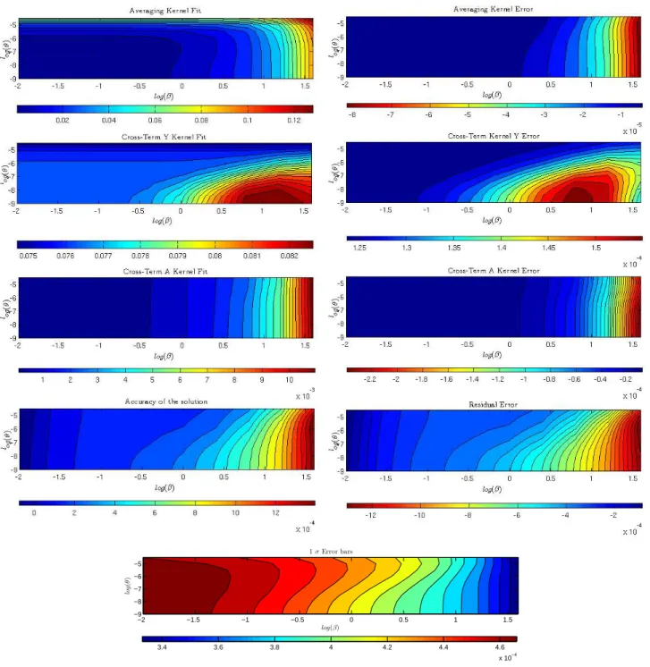
Figure 6.Variations of various quality checks during scan of the β− θ plane for a fixed β2value of 1. (Upper line left)∣∣KAv g− TZ∣∣2, defined in Eq.8, (Upper line right) ǫAv g, defined in Eq.11, (Second line left)∣∣KC r o s s,Y∣∣2, defined in Eq.9, (Second line right) ǫY, defined in Eq.12, (Third line left)∣∣KC r o s s,A∣∣2, defined in Eq.10, (Third line right) ǫA, defined in Eq.13, (Fourth line left) Accuracy of the result, defined as ZT ar− ZI n v, (Fourth line right) ǫR e s, defined in Eq.14, (Lower plot) 1 σ error bars of the inversion results, illustrated here for Ref 3 (The blue regions are associated with smaller errors.).
induced by using the FreeEOS equation of state instead of the Opal equation of state are very small. Indeed, the metal-licity in the enveloppe of this new target is ZC Z = 0.01820 and its helium abundance is YC Z = 0.2386. The inversions
are carried out using the optimal set of trade-off parame-ters given in table3. The inversion results are illustrated in figure 8, where we used circles as the notation for the in-versions on the target using the Opal equation of state and squares for the inversions on the target using the FreeEOS
equation of state. Due to the closeness of the value ZC Z, for both targets, we plotted only one metallicity value to ease the readibility of figure8. Similarly, the error contributions are illustrated in figure9, where we again differentiated the two targets by using different symbols. The kernels fits are also given in table4.
From figure8, we can see that using the same equation of state improves the inversion results for 2 of the 3 models. Analysing the results of table4, we can see that the kernel
0 0.1 0.2 0.3 0.4 0.5 0.6 0.7 0.8 0.9 1 −7 −6 −5 −4 −3 −2 −1 0 1 Position r/R KC r o ss ,A KCross,A(β2= 10−1) KCross,A(β2= 10−2)
Figure 7.Cross-terms from inversions with a differente β2parameter. The red curve, associated with a high β2shows a lower amplitude than the green curve in the convective zone, but a higher amplitude in the radiative zone, where A is non zero.
Table 3.Trade-off parameters values for the hare-and-hounds exercises.
θ β β2 Ref 1,2,3,6,7,12,15,17 10−6 10 1.0 Ref 4,8 10−3 10 10−3 Ref 5 10−3 10−1 10−1 Ref 9 10−3 1 0.1 Ref 10 10−5 10 0.1 Ref 11 10−5 70 0.1 Ref 13 10−8 10 1.0 Ref 14,16 10−6 1.0 0.1 1 2 3 0.014 0.016 0.018 0.02 0.022 Model Number Z Reference models Inverted results Target value
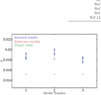
Figure 8. Inversion results for Ref 1, 2 and 3 of the hare and hounds exercises. The blue squares depict inversion results for the target using the FreeEOS equation of state and the blue circles depict the results for the target using the Opal equation of state.
fits have not changed when compared to the values found for the same models in table 2. However, from figure9, it
0 1 2 3 4 −10 −8 −6 −4 −2 0 2 4 6 x 10⁻⁴ Model Number ǫ ǫAvgOpal ǫAvgF reeEOS ǫCross,Y Opal ǫCross,Y F reeEOS ǫCross,AOpal ǫCross,AF reeEOS ǫResOpal ǫResF reeEOS
Figure 9. Error contributions, denoted
ǫAv g,ǫC r o s sY,ǫC r o s s,A,ǫR e s for the hare-and-hounds exer-cises for both targets using Opal and FreeEOS equations of state.
clearly appears that the variation of the results is due to a variation of the residual error for all models. This is expected since it is this error contribution that should be affected by the change in the equation of state. For Refs 1 and 2, ǫRes
is clearly reduced by using the same equation of state in the target and reference model. Yet, the degradation of the results for Ref 3 illustrate that the good quality of the results obtained for the target built with the Opal equation of state might sometimes be fortuitous.
3.2.4 Changing the difference in Z between the hares and the hound
The next step in analysing the behaviour of the inversion is to see how it would behave if smaller metallicity differ-ences were present. Indeed, in the previous test cases, we specifically built our target and reference models such that they showed clear differences in metallicity. Assessing the be-haviour of the inversion if the metallicity is already close is crucial since the real solar case is slightly more complicated. Indeed, metallicity determinations have ranged from 0.0201 in Anders & Grevesse (1989) to 0.0122 in Asplund et al. (2005), with intermediate values found inGrevesse & Noels (1993), Grevesse & Sauval (1998) or Caffau et al. (2011), and one has to be able to assess the stability of the inversion for various differences in metallicity between reference and target. This has already been done to some extent with the four first reference models, which had a higher metallicity of 0.01513in the convective zone.
We now supplement these test cases by carrying out metallicity inversions using Ref 8 and 13 as our new targets. We chose Ref 1 and Ref 4 for respective hounds of Ref 8 and Ref 13. The results are given in table5. They show that smaller changes in metallicity can be seen but the inversion starts to be less reliable. This is expected since the value of the residual error, illustrated in table6, which can go as high as 3×10⁻³. Moreover, as δZ decreases, the importance of the contributions of the other integrals, associated with δY and δ A is increased, and the information on the metallicity is consequently more difficult to extract. However, these exer-cises also show that in such cases, the parameters leading to an accurate inversion result are slightly different than what is found before. Indeed, the parameters were then β = 10, β2= 10−2and θ= 10−3, with the inversion being rather sta-ble around those values, but sometimes showing erratic be-haviour since the contribution from helium or the convective parameter are much higher compared to the contribution of the metallicity in the frequency differences. Thanks to these results, we are now able to assess the quality of the inversion of the real solar metallicity.
4 SOLAR INVERSIONS
4.1 Inverted results and trade-off analysis
Using the parameter sets of table 3 and the analysis per-formed in our hare-and-hounds exercises, we can now carry out inversions on the actual solar data. We used various models calibrated on the Sun as references for the inver-sion. We used the solar radius, luminosity and current value of (ZX)⊙ according to the abundance tables used for the
model as constraints for the solar calibration. We started with models built using the GN93 and AGSS09 abundance tables with multiple combinations of physical ingredients, such as the CEFF or FreeEOS equations of state and the Opal Iglesias & Rogers(1996) or OPLIBColgan et al. (2016) opacity tables, summarised in table7. It should also be noted that Model 5 was built using a uniform reduction of 25% of the efficiency of diffusion, resulting in a higher he-lium abundance and shallower base of the convective zone than Model 1. Similarly, Model 7 was built with an ad-hoc temperature-dependent modification of the diffusion coeffi-cients of the heavy elements that led to significant changes in helium abundance in the convection zone. In addition to this modification, an undershoot of 0.15 of the local pres-sure scale height was added to improve the agreement with the helioseismic determination of the base of the convection zone.
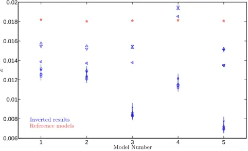
The inversions were carried out for the various combi-nations of parameters found in the hare-and-hounds exer-cises and illustrated in table3. We illustrate in Fig 10the fits of the averaging and cross-term kernels of the inversion, showing that the quality of the inversion in the solar case is comparable to that of the hare-and-hounds exercises. The in-version results are illustrated in Fig11for various reference models identified by their number in abscissa, and where each symbol corresponds to one set of trade-off parameters. Namely, the triangles correspond to the sets associated with higher values of θ and lower values of β2, whereas the other
symbols are associated with values of θ between 10−5 and 10−8.
The first result is that a very large majority of inversions favour a low metallicity, as presented in Vorontsov et al. (2014). Only one small region of the parameter space, for the inversion of Model 4, built with the CEFF equation of state, gives a high metallicity as a solution. However, this solution is not very trustworthy since it is associated with a high cross-term kernel of A. This high cross-term value is a consequence of the parameter set used, which is that of the less stable inversions presented in Sect.3. Inversions of the convective parameter have shown that Model 4 pre-sented large discrepancies with the Sun in its A profile, thus showing the need to damp the the cross-term contribution for this model. When such a damping is realised, the so-lution directly changes to a low-metallicity one. This leads us to consider that these particular results, obtained with a particular parameter set are not to be trusted. Moreover, even for the other models, this set gave higher metallicities, indicating that a systematic error, stemming from the A dif-ferences with the Sun, was potentially re-introduced. Based on these considerations, we consider that the inverted re-sults obtained with this parameter set are not to be trusted. Ultimately, one finds out that the given interval is between [0.008, 0.0014]. While the lowest values of this inversion seem unrealistically low, one should keep in mind that errors of the order of 3.0× 10⁻³ have been observed in the hare-and-hounds exercises, explaining the interval obtained here. This spread is a consequence of the variations in the ingredients of the microphysics in the models, which lead to better or worse agreement with the acoustic structure of the Sun.
Similar tests have been performed with low metallicity AGSS09 models, to assess whether they would favour a high metallicity solar envelope, as in our hare-and-hounds
exer-Table 4.Inversion results for the hare-and-hounds exercises for the target built with the FreeEOS equation of state.
ZR e f ZI n v ∣∣KAv g− TZ∣∣2 ∣∣KC r o s s,Y∣∣2 ∣∣KC r o s s,A∣∣2 Ref 1 0.01513 0.01846± 4.35 × 10⁻⁴ 0.02109 0.07683 5.000× 10⁻³ Ref 2 0.01513 0.01916± 4.26 × 10⁻⁴ 0.02198 0.07680 4.543× 10⁻³ Ref 3 0.01513 0.01757± 4.25 × 10⁻⁴ 0.02169 0.07602 4.549× 10⁻³
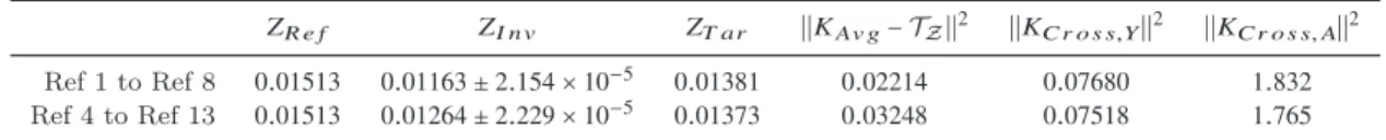
Table 5.Inversion results for the supplementary hare-and-hounds exercises between reference models.
ZR e f ZI n v ZT ar ∣∣KAv g− TZ∣∣2 ∣∣KC r o s s,Y∣∣2 ∣∣KC r o s s,A∣∣2 Ref 1 to Ref 8 0.01513 0.01163± 2.154 × 10⁻⁵ 0.01381 0.02214 0.07680 1.832 Ref 4 to Ref 13 0.01513 0.01264± 2.229 × 10⁻⁵ 0.01373 0.03248 0.07518 1.765
Table 6.Error contributions for the supplementary hare-and-hounds exercises between reference models.
ǫAv g ǫC r o s s,Y ǫC r o s s,A ǫR e s Ref 1 to Ref 8 −3.785 × 10⁻⁷ 2.594× 10⁻⁴ −6.667 × 10⁻⁴ 2.598× 10⁻³ Ref 4 to Ref 13 −4.4674 × 10⁻⁶ −4.301 × 10⁻⁵ −5.289 × 10⁻⁵ 1.197× 10⁻³
cises. The results are quite different. For all parameters sets used in the first sets of hare-and-hounds exercises, the inver-sion gives unrealistic results, ranging from negative metal-licities to values of the order of 0.1 or more, depending on the models and parameter sets. This is not surprising since one infers directly the metallicity difference, δZ, from Eq. 4. This means that if this contribution is very small, it will be dominated by the other differences, δ A and δY. However, in Sect.3, we attempted a few inversions for smaller metal-licity differences between targets and reference models. We showed that in some cases, it was possible to infer the re-sult but that the accuracy was reduced and the cross-term could dominate the results. Using the same parameters as in our supplementary hare-and-hounds exercises, we find that the AGSS09 models place the solar metallicity value around 1.1× 10⁻², which is in agreement with the previous results.
The differences in acoustic structure are expected to be larger between the Sun and the low metallicity stan-dard models than between two numerical models of various metallicities considered in our H&H exercises. Hence, it is not surprising that the inversions performed in our H&H exercises are more successful than real solar inversions of low metallicity standard models. The large differences im-ply larger cross-term contributions, which stem mainly from two regions. The first contribution comes from the radia-tive zone, especially the region just below the convecradia-tive envelope, where the differences in A can be quite large. The second contribution is due to the thin region of the convec-tive envelope where the non-adiabaticity of the convecconvec-tive transport increases and thus A has values strongly differ-ent than 0. Another weakness of low metallicity standard solar models is that they do not reproduce the helium abun-dance in the convective zone. For example, the value found in Model 6 could be different from the solar value by up to 0.025, implying that even if the helium cross-term kernel is strongly damped, it could still strongly pollute the results of the solar inversion. In contrast, the models used in the hare-and-hounds exercises were calibrated to fit the helium value
within an accuracy of 0.01. This problem was less present for Model 7, for which the ad-hoc changes in the ingredients lead to a better agreement with helioseismic constraints and con-sequently, the inversion was slightly more stable. However, the sound speed, density and convective parameter profile inversions still showed larger differences than for GN93 mod-els despite the changes. Therefore, we deem the reliability of the solar inversions from the AGSS09 models, especially that of Model 6, which is particularly unstable, to be less robust and constraining as the inversions from the GN93 models. Therefore we excluded these models from Fig11.
Despite these uncertainties, the indications obtained from these models for a restricted region of the parameter space, combined with the fact that the inversions from GN93 solar models favour a low solar metallicity, still lead us to advocate for a low value of the solar metallicity. However, the precision of this value is quite poor and limited by the intrinsic errors in Γ1 and the uncertainties on the equation
of state. Still, we can conclude that our results do not favour the GN93 abundance tables and any other table leading to similar solar metallicities, like the GS98 or AG89 tables. Had the solar metallicity been that of these abundance tables, a clear trend should have been seen when carrying out solar inversions from low-metallicity AGSS09 models.
4.2 Consequences for solar models
The results presented in section 4.1have significant conse-quences for solar modelling since they confirm the low metal-licity values found byVorontsov et al.(2014). This result im-plies that the observed discrepancies found in sound speed inversions (e.g.Serenelli et al. 2009) are not to be corrected by increasing the metallicity back to former values, but could rather originate from inaccuracies in the physical ingredients of the models. Amongst other, the opacities constitute the physical input of standard solar models that is currently the most uncertain. Recently, experimental determinations of the iron opacity in physical conditions close to those of
Table 7.Properties of the solar models used for the inversion.
Model 1 Model 2 Model 3 Model 4 Model 5 Model 6 Model 7
Mass(M⊙) 1.0 1.0 1.0 1.0 1.0 1.0 1.0 Age(Gy) 4.58 4.58 4.58 4.58 4.58 4.58 4.58 Radius(R⊙) 1.0 1.0 1.0 1.0 1.0 1.0 1.0 L(L⊙) 1.0 1.0 1.0 1.0 1.0 1.0 1.0 YC Z 0.2385 0.2475 0.2445 0.2416 0.2432 0.2292 0.2435 ZC Z 0.01820 0.01803 0.01809 0.01813 0.01805 0.01370 0.01344 (r R)C Z 0.708 0.708 0.711 0.712 0.711 0.718 0.712
Opacity OPLIB OPLIB×1.05 OPLIB OPAL OPLIB OPLIB OPLIB
EOS FreeEOS FreeEOS FreeEOS CEFF FreeEOS FreeEOS FreeEOS
Abundances GN93 GN93 GN93 GN93 GN93 AGSS09 AGSS09
0 0.2 0.4 0.6 0.8 1 −5 0 5 10x 10 −3 Position r/R KC r o ss ,A KCross,A 0 0.2 0.4 0.6 0.8 1 −0.1 0 0.1 0.2 0.3 Position r/R KC r o ss ,Y KCross,Y 0 0.1 0.2 0.3 0.4 0.5 0.6 0.7 0.8 0.9 1 −5 0 5 10 15 20 Position r/R KA v g ,Z KAvg,Z
Figure 10.Same as figure4for a solar inversion.
the base of the solar convective zone have shown discrepan-cies with theoretical calculations of between 30% and 400% (Bailey et al. 2015). The outcome of the current debate (see for example Nahar & Pradhan 2016; Blancard et al. 2016; Iglesias & Hansen 2017, amongst others) in the opacity com-munity that these measurements have caused will certainly influence standard solar models and the so-called “solar mod-elling problem”.
Besides the uncertainties in the opacities, the inade-quacy of the low-metallicity solar models could also result from an inaccurate reproduction of the sharp transition re-gion below the convection zone. In current standard models, this region is not at all modelled, although it is supposed to be the seat of multiple physical processes (seeHughes et al. 2007, for a thorough review) that would affect the tempera-ture and chemical composition gradients, and thus the sound speed profile of solar models.
In addition to these main contributors, further refine-ments of physical ingredients such as the equation of state
(see for exampleBaturin et al. 2013;Vorontsov et al. 2013, for recent studies) or the diffusion velocities could also slightly alter the agreement of low-metallicity solar mod-els and the Sun (see for exampleTurcotte et al. 1998, for a study of the effects of diffusion).
5 CONCLUSION
In this paper, we presented a new approach to determine the solar metallicity value, using direct linear kernel-based inver-sions. We developed in Sect.2an indicator that could allow us to restimate the value of the solar metallicity, provided that the seismic information was sufficient. We showed that the accuracy of the method was limited by intrinsic errors in Γ1 and differences in the equation of state.
In Sect.3, we carried out extensive tests of the inversion technique, using various physical ingredients and reference models. These tests showed that while the inversion could distinguish between various abundance tables such as those
1 2 3 4 5 0.006 0.008 0.01 0.012 0.014 0.016 0.018 0.02 Model Number Z Reference models Inverted results
Figure 11.Inversion results for various solar models. The reference metallicity values are ploted as red☆, while the inverted values are given in blue with each symbol corresponding to a trade-off parameters set. Model 6 and 7 are excluded from the plot (see manuscript for further comment).
of AGSS09 and higher metallicity abundances, like those of GN93 or GS98, it could not be used to determine very ac-curately the value of the solar metallicity, due to intrinsic uncertainties of the method and models.
In Sect. 4, we applied our method on solar data, us-ing the inversion parameters calibrated in the hare-and-hounds exercises carried out previously. We concluded that our method favours a low metallicity value, as shown in Vorontsov et al.(2014). However, further refinements to the technique are necessary to improve the precision beyond that achieved in this study.
Firstly, developing a better treatment of the cross-term contribution from the convective parameter, A, taking into account its 0 value in the convective zone, could help with the analysis of the trade-off problem. Secondly, using other equations of state could help with understanding the un-certainties this ingredient induces on the inversion results. Thirdly, the use of a seismic solar model based on inversions of the A and Γ1profiles as a reference, rather than calibrated
solar models, could reduce the impact of the intrinsic Γ1
er-rors, thus reducing the main contributor to the uncertainties of the inversion and provide more accurate and precise re-sults for this inversion.
ACKNOWLEDGEMENTS
G.B. is supported by the FNRS (“Fonds National de la Recherche Scientifique”) through a FRIA (“Fonds pour la Formation `a la Recherche dans l’Industrie et l’Agriculture”) doctoral fellowship. This article made use of an adapted ver-sion of Inverver-sionKit, a software developed in the context of the HELAS and SPACEINN networks, funded by the Eu-ropean Commissions’s Sixth and Seventh Framework Pro-grammes.
REFERENCES
Anders E., Grevesse N., 1989, Geochimica Cosmochimica Acta,
53, 197
Angulo C., et al., 1999,Nuclear Physics A,656, 3
Antia H. M., Basu S., 1994, A&AS,107
Antia H. M., Basu S., 2006,ApJ,644, 1292
Asplund M., Grevesse N., Sauval A. J., 2005, in Barnes III T. G., Bash F. N., eds, Astronomical Society of the Pacific Confer-ence Series Vol. 336, Cosmic Abundances as Records of Stellar Evolution and Nucleosynthesis. p. 25
Asplund M., Grevesse N., Sauval A. J., Scott P., 2009,ARA&A,
47, 481
Backus G. E., Gilbert J. F., 1967,Geophysical Journal,13, 247
Bailey J. E., et al., 2015, Nature, 517, 3 Basu S., Antia H. M., 1995,MNRAS,276, 1402
Basu S., Antia H. M., 1997,MNRAS,287, 189
Basu S., Chaplin W. J., Elsworth Y., New R., Serenelli A. M., 2009,ApJ,699, 1403
Baturin V. A., Ayukov S. V., Gryaznov V. K., Iosilevskiy I. L., Fortov V. E., Starostin A. N., 2013, in Shibahashi H., Lynas-Gray A. E., eds, Astronomical Society of the Pacific Confer-ence Series Vol. 479, Progress in Physics of the Sun and Stars: A New Era in Helio- and Asteroseismology. p. 11
Blancard C., et al., 2016,Physical Review Letters,117, 249501
B¨ohm-Vitense E., 1958, Z. Astrophys.,46, 108
Brown T. M., Christensen-Dalsgaard J., Dziembowski W. A., Goode P., Gough D. O., Morrow C. A., 1989,ApJ,343, 526
Buldgen G., Reese D. R., Dupret M. A., 2015,A&A,583, A62
Buldgen G., Reese D. R., Dupret M. A., 2017,A&A,598, A21
Caffau E., Ludwig H.-G., Steffen M., Freytag B., Bonifacio P., 2011,Sol. Phys.,268, 255
Cassisi S., Potekhin A. Y., Pietrinferni A., Catelan M., Salaris M., 2007,ApJ,661, 1094
Christensen-Dalsgaard J., Daeppen W., 1992,A&ARv,4, 267
Colgan J., et al., 2016,ApJ,817, 116
Elliott J. R., 1996,MNRAS,280, 1244
Ferguson J. W., Alexander D. R., Allard F., Barman T., Bodnarik J. G., Hauschildt P. H., Heffner-Wong A., Tamanai A., 2005,
ApJ,623, 585
Grevesse N., Noels A., 1993, in Prantzos N., Vangioni-Flam E., Casse M., eds, Origin and Evolution of the Elements. pp 15–25 Grevesse N., Sauval A. J., 1998,Space Sci. Rev.,85, 161
Hughes D. W., Rosner R., Weiss N. O., 2007, The Solar Tachocline
Iglesias C. A., Hansen S. B., 2017,ApJ,835, 284
Iglesias C. A., Rogers F. J., 1996,ApJ,464, 943
Irwin A. W., 2012, FreeEOS: Equation of State for stellar interiors calculations, Astrophysics Source Code Library (ascl:1211.002)
Kosovichev A. G., et al., 1997,Sol. Phys.,170, 43
Nahar S. N., Pradhan A. K., 2016, Physical Review Letters,
116, 235003
Pijpers F. P., Thompson M. J., 1994, A&A,281, 231
Potekhin A. Y., Baiko D. A., Haensel P., Yakovlev D. G., 1999, A&A,346, 345
Reese D. R., Marques J. P., Goupil M. J., Thompson M. J., De-heuvels S., 2012,A&A,539, A63
Rogers F. J., Nayfonov A., 2002,ApJ,576, 1064
Schou J., et al., 1998,ApJ,505, 390
Scuflaire R., Th´eado S., Montalb´an J., Miglio A., Bourge P.-O., Godart M., Thoul A., Noels A., 2008a,Ap&SS,316, 83
Scuflaire R., Montalb´an J., Th´eado S., Bourge P.-O., Miglio A., Godart M., Thoul A., Noels A., 2008b,Ap&SS,316, 149
Serenelli A. M., Basu S., Ferguson J. W., Asplund M., 2009,ApJ,
705, L123
Takata M., Shibahashi H., 2001, in Brekke P., Fleck B., Gurman J. B., eds, IAU Symposium Vol. 203, Recent Insights into the Physics of the Sun and Heliosphere: Highlights from SOHO and Other Space Missions. p. 43
Turcotte S., Richer J., Michaud G., Iglesias C. A., Rogers F. J., 1998,ApJ,504, 539
Vorontsov S. V., Baturin V. A., Ayukov S. V., Gryaznov V. K., 2013,MNRAS,430, 1636
Vorontsov S. V., Baturin V. A., Ayukov S. V., Gryaznov V. K., 2014,MNRAS,441, 3296
This paper has been typeset from a TEX/LATEX file prepared by the author.