TRAVEL TIME EXPENDITURE IN FLANDERS:
TOWARDS A BETTER UNDERSTANDING OF TRAVEL BEHAVIOR
Mario COOLS PhD Candidate
Transportation Research Institute Hasselt University Campus Diepenbeek Wetenschapspark 5 bus 6 3590 Diepenbeek Belgium Tel.: +32(0)11 26 91 31 Fax: +32(0)11 26 91 99 E-mail: mario.cools@uhasselt.be Elke MOONS Post-doctoral Reseacher
Transportation Research Institute Hasselt University Campus Diepenbeek Wetenschapspark 5 bus 6 3590 Diepenbeek Belgium Tel.: +32(0)11 26 91 26 Fax: +32(0)11 26 91 99 E-mail: elke.moons@uhasselt.be Geert WETS Director
Transportation Research Institute Hasselt University Campus Diepenbeek Wetenschapspark 5 bus 6 3590 Diepenbeek Belgium Tel.: +32(0)11 26 91 58 Fax: +32(0)11 26 91 99 E-mail: geert.wets@uhasselt.be
Abstract: In modern societies, mobility is considered to be vital for human
development. In order to lead an efficient policy and achieve environmental goals, governments require reliable predictions of travel behavior. In this paper, the travel time expenditure in Flanders is investigated. The focus is put on the time spent on commuting. Two modeling approaches are used for the analysis of daily travel time expenditure, namely the Poisson regression approach and the classical linear regression approach. In this paper it is shown that socio-demographics, day-effects and transportation preferences are contributing significantly in the explanation of variability in daily commuting time and that multiplicative effects of the transportation preferences form good approximations of the travel time ratios.
Keywords: travel time expenditure, daily commuting time, holiday effects, (Poisson)
TRAVEL TIME EXPENDITURE IN FLANDERS:
TOWARDS A BETTER UNDERSTANDING OF TRAVEL BEHAVIOR
1. INTRODUCTION
In modern societies, mobility is considered to be vital for human development: mobility is not only regarded as one of the driving forces behind economic growth, but also seen as a social need that offers people the opportunity for self-fulfillment and relaxation (Ministerie van Verkeer en Waterstaat, 2004). Reports from various international organizations, like for instance the European Commission’s White paper “European transport policy for 2010: time to decide” (European Commission, 2004) indicate that governments acknowledge the essential role that mobility plays.
In order to lead an efficient policy and achieve environmental goals, such as the Kyoto norms, governments require reliable predictions of travel behavior. A better understanding of travel behavior will lead to better forecast and thus policy measures can be fine-tuned based on more accurate data.
In this paper, the travel time expenditure in Flanders (the Dutch speaking part of Belgium) is investigated. The focus is put on the time spent on commuting, where commuting trips are defined as school- and work-related trips. Travel behavior researchers have regained interest in the travel time budget (the daily travel time expenditure) in the context of activity-based and time use research in travel behavior modeling (Banerjee et al., 2007). The notion of a constant travel time budget is thoroughly discussed in the literature (van Wee et al., 2006).
2. OVERVIEW OF THE DATA
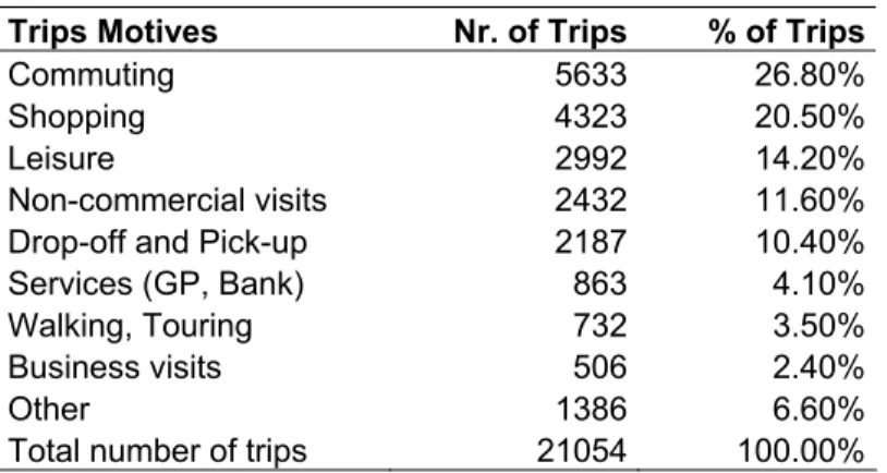
The data that will be used for the analysis stem from a household travel survey in Flanders that was carried out in 2000 (Zwerts and Nuyts, 2002). The focus of this survey was to investigate the travel behavior of the people living in the Flanders area. Since commuting was the primary motive for travel, as can be seen from Table 1, this paper focuses on investigating the daily time expenditure on commuting.
Table 1: Categorization of trips according to trip motive
Trips Motives Nr. of Trips % of Trips
Commuting 5633 26.80%
Shopping 4323 20.50%
Leisure 2992 14.20%
Non-commercial visits 2432 11.60% Drop-off and Pick-up 2187 10.40%
Services (GP, Bank) 863 4.10%
Walking, Touring 732 3.50%
Business visits 506 2.40%
Other 1386 6.60%
2.1 Daily commuting time
The daily commuting time is calculated by adding up the time spent on school- or work-related travel. Both the trips to the work/school locations and the trips back home were considered to be commuting trips. For this calculation all the respondents, that made at least one trip during the survey period (not necessarily a commuting trip), were considered. Figure 1 displays the distribution of the daily commuting times. Note that more than half of the respondents did not commute at all. The average time that the respondents spent on commuting was about 21 minutes.
Figure 1: Distribution of Daily Commuting Time
2.2 Socio-demographics
Socio-demographic variables are commonly used in models that predict travel time (Frusti et al., 2002, Sall, et al., 2007). The following variables are used for the analysis presented in this paper: age, sex, and employment status. When Tables 2(a) and 2(b) are explored it can be seen that the daily commuting first increases with age, reaches his maximum at age category 35-44 and declines after people reach their retirement age. The daily commuting team seems to be a lot higher for males than for females and obviously the professionally active population spends more time on commuting compared to the inactive population.
Table 2(a): Descriptive statistics of age
Daily Commuting Time (in minutes) Variable Mean St. Deviation Nr of obs.
Age 6-12 12.38 22.27 550 13-15 23.10 29.19 242 16-24 28.26 40.73 788 25-34 28.76 46.40 844 35-44 29.07 50.38 1169 45-54 25.43 52.39 1074 55-64 11.44 35.43 786 65+ 1.41 12.59 608
Table 2(b): Descriptive statistics of sex and employment status
Daily Commuting Time (in minutes) Variable Mean St. Deviation Nr of obs.
Sex Male 26.05 50.58 3134 Female 16.53 31.90 2919 Employment status Housekeeping 0.68 5.89 401 Unemployed 2.57 10.57 179 Retired 1.33 15.16 881 Disabled 1.47 6.53 97 Pupil, Student 20.16 32.96 1348 Worker 31.04 48.93 912 Employee 33.29 53.71 1335 Executive 42.14 58.73 448 Liberal Profession 14.00 23.77 67 Self-Employed 24.43 46.13 261 Other, Non-Occupational 4.52 14.08 25 Other, Occupational 19.64 28.22 28 2.3 Day-effects
Next to the demographic variables, also some day-effects are used for the analysis. Day-of-week effect
Agarwal (2004) showed that there exists a significant difference between travel behavior on a weekday and travel behavior on a weekend day. This difference is even further unraveled by Sall and Bhat (2007) demonstrating a significant day-of-week effect. For the analysis the day-of-week effect is represented in a categorical variable with seven categories; the first category corresponding to a Monday, the last to a Sunday.
Holiday effect
Liu and Sharma (2006) and Cools et al. (2007) indicated the importance of incorporating holiday effects into travel behavior models. To evaluate the significance of holidays on daily commuting time a special holiday variable is created, consisting of three categories: “normal days”, “holidays” and “summer holidays”. The following holidays are taken into account: Christmas vacation, spring half-term, Easter vacation, Labor Day, Ascension Day, Whit Sunday, Whit Monday, vacation of the construction industry (three weeks, starting the second Monday of July), Our Blessed Lady Ascension, fall break (including All Saints’ Day and All Souls’ Day), and finally Remembrance Day. Note that for all these holidays, the adjacent weekends, were considered to be a holiday too. For holidays occurring on a Tuesday or on a Thursday, respectively the Monday and weekend before, and the Friday and weekend after, were also defined as a holiday, because often people have a day-off at those days, and thus have a leave of several days, which might be used to go on a long weekend or on a short holiday (Cools et al., 2007) The days in July and August that were not in the above holiday list were labeled as “summer holidays”.
2.4 Transportation preferences
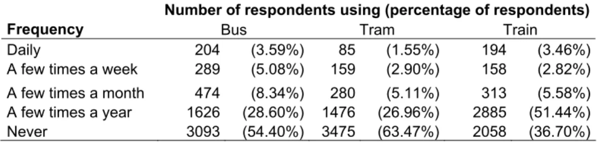
A final group of variables that is used for the analysis is the use of public transport services. The following transport services were considered: the use of the scheduled service bus, the use of the tramway service and use of the railroad system. As can be noted from Table 3, more than half of the respondents never use busses or trams. The use of trains is slightly more popular.
Table 3: Descriptive statistics for the use of public transport services
Number of respondents using (percentage of respondents)
Frequency Bus Tram Train
Daily 204 (3.59%) 85 (1.55%) 194 (3.46%)
A few times a week 289 (5.08%) 159 (2.90%) 158 (2.82%) A few times a month 474 (8.34%) 280 (5.11%) 313 (5.58%) A few times a year 1626 (28.60%) 1476 (26.96%) 2885 (51.44%)
Never 3093 (54.40%) 3475 (63.47%) 2058 (36.70%)
3. METHODOLOGY
Two modeling approaches are used for the analysis of daily travel time expenditure, namely the Poisson regression approach and the classical linear regression approach. The Poisson regression approach is defended by arguing that time expenditure can never take negative values. The classical linear regression approach can be justified by claiming that there is a widespread and continuous range of values that the travel time expenditure can adopt. This wide range is also witnessed from Figure 1. Comparing linear regression models with Poisson regression models is not a straightforward task. Therefore an objective criterion is constructed to compare the two types of models.
3.1 Exploratory data analysis: Regression tree
To get prior insight into the data, a regression tree is built through a process known as binary recursive partitioning. This is an iterative process of splitting the data into two partitions, and then splitting it up further on each of the branches. The algorithm chooses the split that partitions the data into two parts such that it minimizes the sum of the squared deviations from the mean in the separate parts. This splitting (or partitioning) is then applied to each of the new branches. The process continues until a saturated tree is grown. A tree is saturated in the sense that the nodes subject to further division cannot be split (Therneau and Atkinson, 1997). The terminal nodes are then recombined or “pruned” upwards to an optimal size tree. The degree of pruning is determined by cross-validation using a cost-complexity function that balances the apparent error rate with the tree-size. The optimal tree is the tree that corresponds to the complexity parameter that gives a minimum cost for the new data (Breiman et al., 1984). Since no separate test sample was available, V-fold cross-validation was used as an alternative. A specified V value determines the number of random sub samples, as equal in size as possible, that is formed from the learning sample. The binary tree is then computed V times, each time leaving out one of the sub samples from the calculations. The sub sample that was not used in the calculations serves then as a test sample for cross-validation (CV). The CV costs computed for each of the V test samples are then averaged to give the V-fold estimate of the CV cost.
3.2 ‘Classical’ linear regression
The classical linear regression approach is a modeling philosophy that tries to explain the dependent variable with the help of other covariates. Formally, the multiple linear regression model can be represented by the following equation:
Yi = β0 + β1Xi,1 + β2Xi,2 + … + βp-1Xi,p-1 + εi (1)
where Yi is the i-th observation of the dependent variable, Xi,1, Xi,2, …, Xi,p-1 the
corresponding observations of the explanatory variables, β0, β1, β2,…, βp-1 the
parameters, which are fixed, but unknown, and where εi is the unknown random error.
Estimates for the unknown parameters can be obtained by classical estimation techniques. If b0, b1, b2, …, bp-1 are the estimates for the parameters, then the
estimated value for the dependent variable Yi is given by:
Ŷi = bo + b1Xi,1 + b2Xi,2 + … + bp-1Xi,p-1 (2)
The following assumptions are made about the explanatory variables and the error terms.
• The error terms must be uncorrelated with the explanatory variables. If one of the explanatory variables is correlated with the error terms, it means that that covariate is correlated with unmeasured variables that are influencing the dependent variable.
• The assumption of homoskedasticity: the error terms must have the same variance for all values of the explanatory variables. Thus the predicted values of the independent variable must be equally good for all values of the explanatory variables.
• The values of the error terms have to be independent of one another. Non-independence leads to autocorrelation. This occurs when unmeasured variables are systematically similar between some pairs of observations.
• The error terms must be normal distributed. If the error terms are not normally distributed, the parameter estimate is usually also not normally distributed and thus the desirable characteristics of a normally distributed estimate would no longer be true.
• Absence of multicollinearity. The estimated parameter coefficients will be unstable and unreliable if explanatory variables are highly correlated. In the presence of multicollinearity, the effect of a single explanatory variable cannot be isolated, as the regression coefficients are quite uninformative and their confidence intervals very wide.
When these assumptions are satisfied, then the estimators for the parameters are BLUE (Best Linear Unbiased Estimators). Otherwise some remedial measures, like transformations, are required (Neter et al., 1996).
3.3 Poisson regression
Explaining a dependent variable by means of other covariates is also the hands-on approach in Poisson regression. Instead of assuming independent normal distributed error terms like the classical linear regression approach, the Poisson regression technique is based on the assumption that the dependent variable is Poisson distributed. Formally, the model can be represented in the following way:
(
)
2 2 2 2 6 1 1 i i d n n ⎛ ⎞ ⎜ ⎟ Ψ = −⎜ ⎟ − ⎜ ⎟ ⎝ ⎠∑
or equivalently:E[Yi]) = exp(β0 + β1Xi,1 + β2Xi,2 + … + βp-1Xi,p-1) (4)
where E[Yi] is the expected value of the i-th observation of the dependent variable,
Xi,1, Xi,2, …, Xi,p-1 the corresponding observations of the explanatory variables, and β0,
β1, β2,…, βp-1 the parameters (Agresti, 2002). Estimates for the unknown parameters
are obtained by maximizing the log likelihood using a ridge-stabilized Newton-Raphson algorithm (SAS Institute Inc., 2004).
The assumption of a Poisson distribution entails that the mean and variance of the presumed Poisson distributed variable must be (quasi-)equal. When the variance is significantly higher there is a problem of overdispersion. Potential overdispersion is taken into account by using the deviance as a dispersion parameter. Note that function obtained by dividing the log-likelihood function by the dispersion parameter is not a legitimate log-likelihood function, but a quasi-likelihood function. Nevertheless, most of the asymptotic theory for log-likelihoods also applies to quasi-likelihoods (McCullagh and Nelder, 1989).
3.4 Model comparison criterion
Comparing linear regression models with Poisson models is not a straightforward task. An objective criterion is needed to assess the performance of the two model approaches. Starting point is the determination coefficient (R²) that is used in linear regression. This R² can be defined as the squared value of the Pearson correlation between the predicted values and the dependent variable. However, the Pearson correlation requires that the predicted values and the dependent variable are bivariate normally distributed. In classical linear regression this assumption is fulfilled when the residuals are normally distributed. However for Poisson models this assumption seems inappropriate. Therefore the Spearman correlations, which are non-parametric correlation estimates, form a more defendable basis for a comparison criterion. The new criterion, the Spearman Determination coefficient (Ψ²), is defined as the square of the Spearman Correlation coefficient between the predicted and real values of the dependent variable. Formally the Spearman Determination coefficient can be represented in the following way:
(5)
where di is the difference between each rank of corresponding predicted and real
values, and where n equals the number of observations (Cohen and Cohen, 1983).
4. RESULTS
4.1 Exploratory data analysis
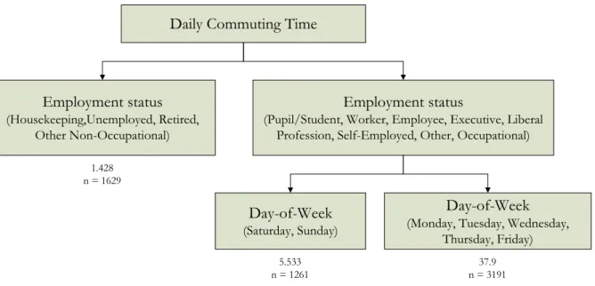
The regression tree that is built through binary recursive partitioning is given in Figure 2. This tree is the pruned tree that takes into account a complexity parameter (cp) of 0.02548, minimizing the cost for new data. This cost was calculated by cross validation using 10 subsamples. Note that if fewer than 10 cross validations would have been used, the error rate of the tree could have been seriously overestimated (Breiman et al, 1984).
Figure 2: Binary regression tree for the daily commuting time
Figure 2 reveals that the employment status is the most important discriminator in explaining daily commuting time. As expected, the active population spends more time on commuting than their inactive counterpart. Next to the employment status, also day-of-week effects seem to be determining the daily communing time: during weekends people spent less time on going to work/school than during weekdays. Quite obviously this can be explained by the fact that most people only work during weekdays.
4.2 Linear regression
The variables that were used in the final linear regression model, together with their likelihood ratio (LR) statistics are displayed in Table 4. From this Table, it can be seen that all three categories of variables (socio-demographic variables, day effects and transportation preferences) are contributing significantly in the unraveling of daily travel time. The age effect, although insignificant, was kept in the model, because of the significant interaction effect between gender and age. Remind that p-values of interaction effects only have a valid interpretation when also the main effects are included in the model (Neter et al, 1996).
Table 4: LR Statistics (Type 3) For Linear Regression
Variable DF Chi-Square P-value
Holiday 2 57.51 < 0.0001 Day-of-week 6 138.12 < 0.0001 Interaction Holiday/Day-of-week 12 32.19 0.0013 Age 7 5.45 0.6051 Sex 1 21.57 < 0.0001 Interaction Age/Sex 7 52.28 < 0.0001 Employment Status 11 239.50 < 0.0001 Scheduled service bus 4 53.12 < 0.0001
Tramway service 4 18.54 0.0010
Railroad system 4 118.79 < 0.0001
Daily Commuting Time
Employment status (Housekeeping,Unemployed, Retired,
Other Non-Occupational)
Employment status
(Pupil/Student, Worker, Employee, Executive, Liberal Profession, Self-Employed, Other, Occupational)
Day-of-Week (Saturday, Sunday)
Day-of-Week (Monday, Tuesday, Wednesday,
Thursday, Friday) 1.428 n = 1629 5.533 n = 1261 37.9 n = 3191
Table 5(a) shows the parameter estimates for the Linear Regression model. These Linear Regression parameter estimates can be interpreted as additive effects. If for instance the parameter estimates for Workers and Employees are compared, then the additive effect of being and employee instead of a worker can be calculated by a simple subtraction: 29.3025 – 25.9094 = 3.3931. This means that employees spent on average 3.3931 minutes more on daily commuting time than workers do, given that they share the same characteristics for the other variables.
By examining part a of the table, it can be seen that the active population obviously spends more time on commuting than the inactive population. The higher the position within a company, the more daily time is spent on commuting. Correspondingly, executives spend the most time on commuting. Also important to notice, is that people who use public transport (bus, train, tram) commute longer than the ones who seldom or never use public transport (20 up to 33 minutes longer).
Table 5(a): Parameter estimates for linear regression model
Parameter Estimate Parameter Estimate
Intercept -20.2705 Use of scheduled service bus Employment status Daily 23.5018
Housekeeping 5.9466 A few times a week 3.3912
Unemployed 0 A few times a month 2.2725
Retired 0.5872 A few times a year 0.8242
Disabled -0.9767 Never 0
Pupil, student 14.1228 Use of tramway service
Worker 25.9094 Daily 19.5191
Employee 29.3025 A few times a week -0.7410 Executive 34.3036 A few times a month 1.9913 Liberal Profession 11.3672 A few times a year 0.7206
Self-employed 18.5779 Never 0
Other, Non-Occupational 7.2682 Use of train
Other, Occupational 18.3512 Daily 30.9260 A few times a week 14.9523 A few times a month -3.3527 A few times a year -1.1999
Never 0
Table 5(b): Total Effects for Day-of-week x Holiday Status
Holiday Status
Day-of-week Normal day Holiday Summer Holiday
Monday 29.9273 19.2130 13.4156 Tuesday 32.1461 23.9021 13.6732 Wednesday 26.8283 19.6896 12.2422 Thursday 30.9206 9.4924 18.4244 Friday 25.0761 14.9622 16.4569 Saturday 1.7512 1.0133 -1.5522 Sunday 0 -2.5585 3.6116
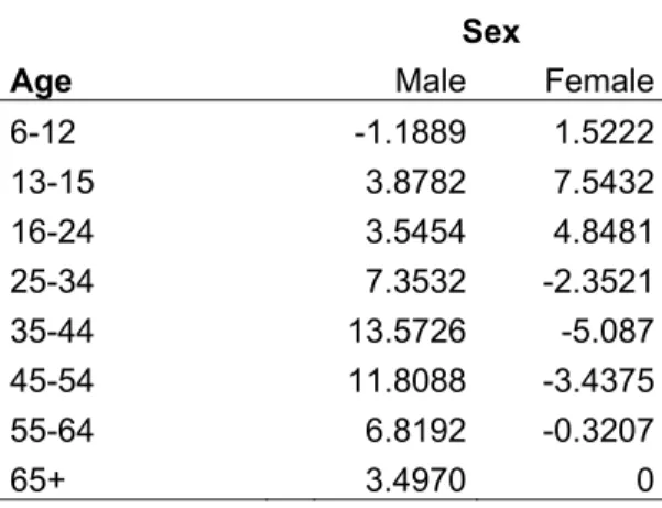
Part b and c of the table give the parameter estimates of the total effects for respectively day-of-week and holiday status, and age and sex. Note that these total effects are calculated by adding up the parameter estimates for both main effects and the interaction effect. From Part b of the table it can be seen that during holidays, summer holidays and weekends people spent much less time on commuting than during normal weekdays. Part c of the table indicates that young females (06-24) commute longer than there peer males, while elder males (25+) commute longer than there females counterparts.
Table 5(c): Total Effects for Age x Sex
Sex
Age Male Female
6-12 -1.1889 1.5222 13-15 3.8782 7.5432 16-24 3.5454 4.8481 25-34 7.3532 -2.3521 35-44 13.5726 -5.087 45-54 11.8088 -3.4375 55-64 6.8192 -0.3207 65+ 3.4970 0 4.3 Poisson regression
Table 6 displays the variables that were used in the Poisson regression model. To ease comparison between the two types of models, the same variables were taken into account as the linear regression model. From Table 6, one could observe that all three categories of variables (socio-demographic variables, day effects and transportation preferences) are playing a significantly role in the interpretation of daily travel time. Contrary to the linear regression model, the main age effect has a significant meaning in the Poisson regression model.
Table 6: LR Statistics (Type 3) For Poisson Regression
Variable DF Chi-Square P-value
Holiday 2 54.85 < 0.0001 Day-of-week 6 492.48 < 0.0001 Interaction Holiday/Day-of-week 12 31.33 0.0018 Age 7 43.87 < 0.0001 Sex 1 34.17 < 0.0001 Interaction Age/Sex 7 90.00 < 0.0001 Employment Status 11 836.44 < 0.0001 Scheduled service bus 4 65.62 < 0.0001
Tramway service 4 20.20 0.0005
Railroad system 4 124.08 < 0.0001
The parameter estimates for the Poisson Regression model are shown in Table 7(a). These parameter estimates should be interpreted as multiplicative effects. Take as an example the parameter estimates for Workers and Employees. The multiplicative effect of being and employee instead of a worker can then be calculated in the
following way: exp(2.3989 – 2.2852) = exp(0.1137) = 1.1204. This means that employees are commuting on average 1.1204 times longer (in terms of duration) than workers.
Table 7(a): Parameter Estimates For Poisson Regression Model
Parameter Estimate Parameter Estimate Intercept -3.6835 Use of scheduled service bus
Employment status Daily 0.6008
Housekeeping -1.1669 A few times a week 0.1356
Unemployed 0 A few times a month 0.0811
Retired -0.2939 A few times a year 0.0346
Disabled -0.5122 Never 0
Pupil, student 1.8745 Use of tramway service
Worker 2.2852 Daily 0.4205
Employee 2.3989 A few times a week 0.0531 Executive 2.4739 A few times a month 0.0657 Liberal Profession 1.5340 A few times a year 0.0694
Self-employed 2.0230 Never 0
Other,
Non-Occupational 0.7433 Use of train
Other, Occupational 1.9887 Daily 0.5533
A few times a week 0.4600 A few times a month -0.1808 A few times a year -0.0789
Never 0
From part a of the table, it can be seen that the occupationally active people quite logically spend more time on commuting than occupationally inactive people. The higher the position people hold within a company, the more daily time they spend on commuting. Hence, similar results are obtained when compared to the classical regression model.
Another point that requests attention is the fact that people who use public transport (bus, train, tram) commute 1.52 (=exp(0.4205-0)) up to 1.88 (=exp(0.5533+0.0789)) times longer than the ones who seldom or never use public transport. Interesting is that these parameter estimates could be seen as approximations of the travel time factors, which are defined as ratios of the time spent for a certain trajectory using public transport to the time spent using a car. When these approximations are compared to the total travel time factor of 1.7 reported in the Flemish Mobility Plan (Ministerie van de Vlaamse Gemeenschap, 2001), one can conclude that the approximations work reasonable well and provide a more thorough look at the subject of travel time factor.
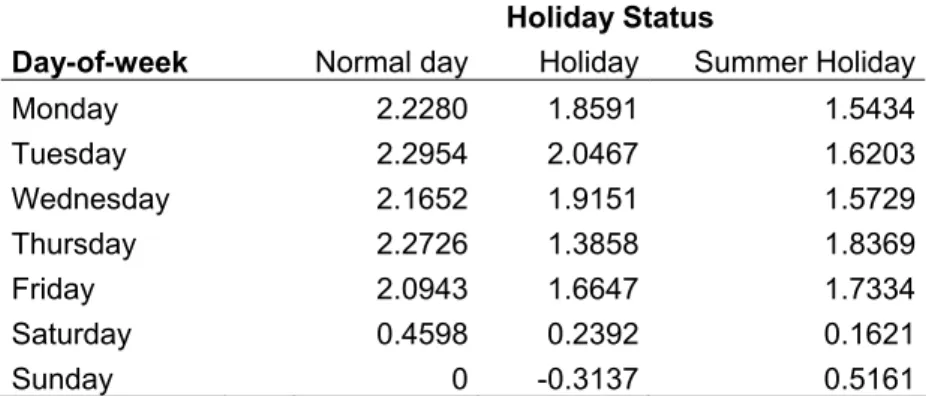
The parameter estimates of the total effects for respectively day-of-week and holiday status, and age and sex are given in Part b and c of the table. Remind that these total effects are calculated by adding up the parameter estimates for both main effects and the interaction effect. Part b of the table illustrates that during holidays, summer holidays and weekends people spent much less time on commuting than
during normal weekdays. From Part c of the table on can notice that young females (06-24) commute longer than there peer males, while elder males (25+) commute longer than there females counterparts.
Table 7(b): Total Effects for Day-of-week x Holiday Status
Holiday Status
Day-of-week Normal day Holiday Summer Holiday
Monday 2.2280 1.8591 1.5434 Tuesday 2.2954 2.0467 1.6203 Wednesday 2.1652 1.9151 1.5729 Thursday 2.2726 1.3858 1.8369 Friday 2.0943 1.6647 1.7334 Saturday 0.4598 0.2392 0.1621 Sunday 0 -0.3137 0.5161
Table 7(c): Total Effects for Age x Sex
Sex
Age Male Female
6-12 2.4047 2.5902 13-15 2.8718 3.0582 16-24 2.9321 2.9675 25-34 2.9882 2.6980 35-44 3.1630 2.4991 45-54 3.1886 2.5815 55-64 3.1480 2.6078 65+ 2.7993 0 4.4 Model comparison
When the linear regression model is compared with the logistic regression model it is important to acknowledge that both model approaches yield consistent findings. One of the most important variables in explaining differences in daily commuting time is the employment status. Also Craviolini (2006) stressed the importance of this social status. Next to the employment status, the other socio-demographic variables that were taken into account, namely Age and Sex, were contributing significantly in explaining variability in daily commuting time. These findings are coherent with international literature on this subject (Bhat and Misra, 1999, Kapur and Bhat, 2007). Findings concerning the significant day-of-week effects and holiday effects were harmonious with the results reported in Lockwood et al. (2005) and Cools et al. (2007).
Table 8: Spearman Determination coefficient (Ψ²)
Model Type CorrelationSpearman Ψ² (Psi-square)
Poisson regression 0.66395 0.441 Linear regression 0.62344 0.389
Table 8 shows the Spearman Determination coefficient (Ψ²) that can be used to assess the performance of the two model approaches. From this table one can see that this coefficient is higher for the Poisson regression and consequentially one can conclude that Poisson regression modeling is the approach to be preferred when trying to explain daily commuting time. The fact that the Linear regression model yielded both negative and positive values for the daily commuting time predictions, while the Poisson regression model only yielded positive values, favors the Poisson regression even more.
5. CONCLUSIONS AND FURTHER RESEARCH
In this paper it is shown that socio-demographics, day-effects and transportation preferences are contributing significantly in the explanation of variability in daily commuting time. Both the linear regression approach and the Poisson regression approach yielded findings that were consistent with international literature. When the performance of the two model approaches is evaluated, the Spearman Determination Coefficient favored the Poisson regression approach.
On of the most appealing results of this study is the fact that people who often use public transport (buses, trams or trains) spend more time on commuting than there counterparts who avoid using public transport services. An important question that could be raised is why these people still choose in favor of public transport: because of ease, comfort, safety? A stated-preference research might give an answer to this. Since commuting trips consume the largest part of the travel time expenditure, it is essential that policy makers acknowledge these findings. An essential step for stimulating the modal split, and thereby trying to achieve reliable travel times and environmental goals, such as the Kyoto norms, is the continuation of investments in public transport. Only when “acceptable” travel times are achieved by the public transport services, the general public will consider switching their transport mode. Choosing for those investments that reduce public transport travel times thus is a key challenge for policy makers.
In this paper it was evidenced that the multiplicative effects of the transportation preferences form good approximations of the travel time ratios. Thus, the reported Poisson methodology offers a framework that can be used to fine-tune policy measures.
Further investigation on other types of travel time expenditure (e.g. daily travel time expenditure on shopping or leisure) is necessary to realize a deeper understanding of Flemish travel behavior. Incorporation of other covariates, such as degree of urbanization, might even further illuminate the insights in travel behavior.
REFERENCES
a) Books and Books chapters
Agresti, A. (2002) Categorical Data Analysis, Second Edition, Wiley, Hoboken, NJ. Breiman, L., Friedman, J.H., Olsen, R.A. and Stone, C.J. (1984) Classification and
regression trees, Wadsworth, Belmont.
Cohen, J. and Cohen, P. (1983) Applied multiple regression/correlation analysis
for the behavioral sciences, Second Edition, Erlbaum, Hillsdale, NJ.
McCullagh, P. and Nelder, J.A. (1989) Generalized Linear Models, Second Edition, Chapman and Hall, London.
Neter, J., Kutner, M.H., Nachtsheim, C.J. and Wasserman, W. (1996) Applied
Linear Statistical Models, Fourth Edition, WCB/McGraw-Hill, Burr Ridge, Illinois.
SAS Institute Inc. (2004) SAS/STAT 9.1 User’s Guide, SAS Institute Inc., Cary, NC. b) Journal papers
Banerjee, A., Ye, X. and Pendyala, M. (2007) Understanding travel time expenditures around the world: exploring the notion of a travel time frontier, Transportation, Vol.
34, No. 1, 51-65.
Bhat, C.R. and Misra, R. (1999) Discretionary activity time allocation of individuals between in-home and out-of-home and between weekdays and weekends,
Transportation, Vol. 26, No. 2, 193-209.
Cools, M., Moons, E. and Wets, G. (2007) Investigating the Effect of Holidays on Daily Traffic Counts: A Time Series Approach, Transportation Research Record:
Journal of the Transportation Research Board, Forthcoming.
Frusti, T., Bhat, C.R. and Axhausen, K.W. (2002) Exploratory Analysis of Fixed Commitments in Individual Activity-Travel Patterns, Transportation Research
Record: Journal of the Transportation Research Board, No. 1807, 101-108.
Liu, Z. and Sharma, S. (2006) Predicting Directional Design Hourly Volume from Statutory Holiday Traffic, Transportation Research Record: Journal of the
Transportation Research Board, No. 1968, 30-39.
Lockwood, A.M., Srinivasan, S. and Bhat, C.R. (2005) Exploratory Analysis of Weekend Activity Patterns in the San Francisco Bay Area, California, Transportation Research Record: Journal of the Transportation Research
Board, No. 1926, 70-78.
Sall, E.A. and Bhat, C.R. (2007) An analysis of weekend work activity patterns in the San Francisco Bay Area, Transportation, Vol. 34, No. 2, 161-175.
Wee, B.v., Rietveld, P. and Meurs H. (2006) Is average daily travel time expenditure constant? In search of explanations for an increase in average travel time, Journal
c) Papers presented at conferences
Craviolini, C. (2006) Commuting Behaviour as Part of Lifestyle, 6th Swiss Transport
Research Conference, Monte Verità / Ascona, Switzerland, March 15-17, 2006.
Kapur, A. and Bhat, C.R. (2007) On Modeling Adults’ Weekend Day Time Use by Activity Purpose and Accompaniment Arrangement, Proceedings of the 86th
Annual Meeting of the Transportation Research Board, Washington, DC, USA,
January 21-25, 2007. d) Other documents
Agarwal, A. (2004) A Comparison of Weekend and Weekday Travel Behaviour
Characteristics in Urban Areas, Master Thesis, University of South Florida, Tampa.
European Commission (2001) White Paper on European Transport Policy 2010:
Time to Decide. Office for Official Publications of the European Communities,
Luxemburg.
Ministerie van de Vlaamse Gemeenschap (2001) Ontwerp Mobiliteitsplan
Vlaanderen, Departement Leefmilieu en Infrastructuur, Mobiliteitscel, Brussel.
Ministerie van Verkeer en Waterstaat (2004) Nota Mobiliteit. Ministerie van Verkeer en Waterstaat, Den Haag.
Therneau, T.M. and Atkinson, E.J. (1997) An introduction to Recursive
Partitioning Using the RPART Routines, Mayo Foundation, Jacksonville. Online
available at: http://www.mayo.edu/hsr/techrpt/61.pdf.
Zwerts, E. and Nuyts, E. (2002) Onderzoek Verplaatsingsgedrag Vlaanderen
(januari 2000 – januari 2001), Deel 3A: Analyse personenvragenlijst, Provinciale