Transport Methods for the Numerical Computation
of Nonlinear Normal Modes
L. Renson1, F. Blanc2, C. Touzé2, G. Kerschen1 1
Space Structures and Systems Laboratory, Aerospace and Mechanical Engineering Department, University of Liège, 1 chemin des Chevreuils, 4000 Liège, Belgium 2
ENSTA-UME, Unité de Recherche en Mécanique, ENSTA-ParisTech Chemin de la Hunière, 91761 Palaiseau Cedex, France
During the last decade, various numerical techniques for computing nonlinear normal modes (e.g., the harmonic balance method and the continuation of periodic solutions) have emerged to overcome the inherent limitations of analytical techniques. The development of such algorithms paves the way for the computation of NNMs of large-scale, real-life applications. However, most existing computational methods consider conservative systems. If the effect of weak damping can often be considered as purely parasitic, this no longer holds for systems with moderate or high damping or with nonlinear damping.
Shaw and Pierre extended the definition of an NNM to nonconservative systems; an NNM is defined as an invariant manifold in phase space. Based on the center manifold technique, they derived a set of partial differential equations (PDEs) governing the manifold’s geometry. These equations were first solved analytically using series expansion and then numerically by a Galerkin approach. Specifically, the PDEs were solved using global shape functions defined over the entire domain.
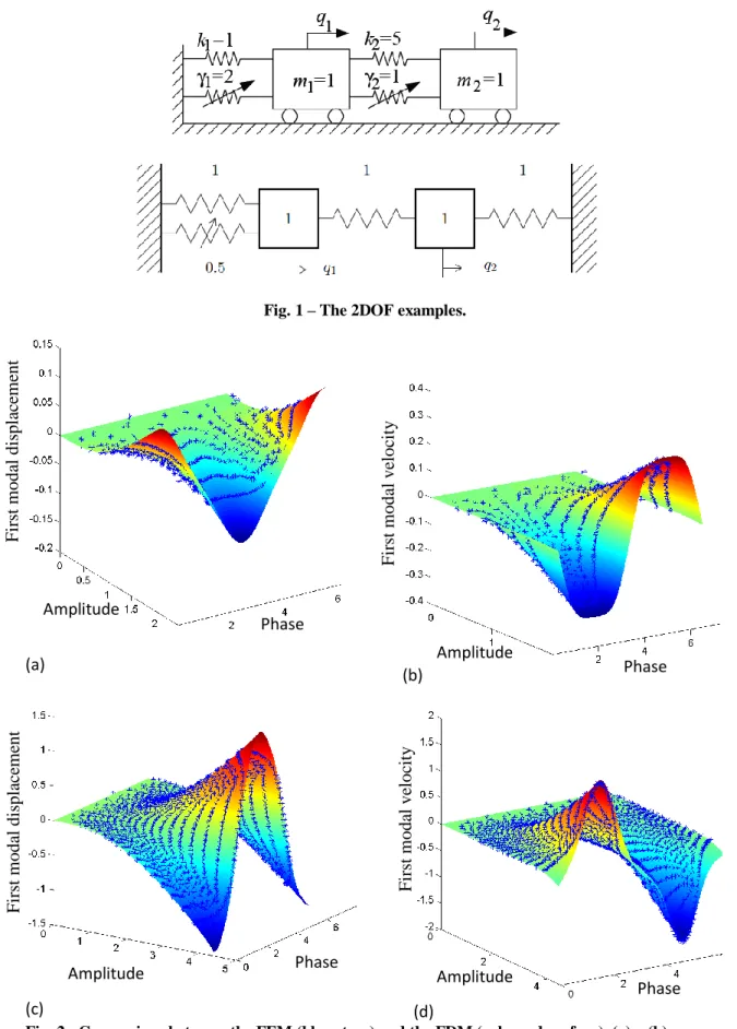
To consider applications with larger number of DOFs, this study proposes two different numerical methods that discretize the entire computational domain for solving the PDEs governing the NNM. Due to the hyperbolic nature of the PDEs (i.e., they can be interpreted as the equations of a transport problem), particular care is needed when solving these equations. The first method relies on a finite element (FE) discretization of the computation domain and considers a streamline upwind Petrov Galerkin (SUPG) formulation. The second method uses finite differences (FD) together with an optimization method on the initial conditions. The differences between FD and FE formulations are investigated, and the methods are demonstrated using two 2DOF examples (Figures 1-2). In the conservative case, a comparison with the solutions obtained using the continuation of periodic solutions is performed. Additional comparisons with the previously-developed Galerkin approach are provided. The methods are then applied to a higher-dimensional example. Finally, the extension of both methods to nonconservative systems is discussed.
Fig. 1 – The 2DOF examples.
(a)
(b)
(c) (d)
Fig. 2 - Comparison between the FEM (blue stars) and the FDM (coloured surface). (a) – (b) Second NNM for the first 2DOF system in Fig. 1. (c) – (d) Second NNM for the second 2DOF system in Fig. 1. F ir st m oda l di spl ac em ent Amplitude Phase Amplitude Phase F ir st m oda l ve loc it y Amplitude Phase Amplitude Phase F ir st m oda l ve loc it y F ir st m oda l di spl ac em ent