To cite this document:
Zhang, Siyuan and Zenou, Emmanuel A Caustic Approach of
Panoramic Image Analysis. (2010) In: Advanced Concepts for Intelligent Vision
Systems, 13 December 2010 - 16 December 2010 (Sydney, Australia).
O
pen
A
rchive
T
oulouse
A
rchive
O
uverte (
OATAO
)
OATAO is an open access repository that collects the work of Toulouse researchers and
makes it freely available over the web where possible.
This is an author-deposited version published in:
http://oatao.univ-toulouse.fr/
Eprints ID: 11294
Any correspondence concerning this service should be sent to the repository
administrator:
staff-oatao@inp-toulouse.fr
A Caustic Approach of Panoramic Image
Analysis
Siyuan Zhang and Emmanuel Zenou
Universit´e de Toulouse
Institut Sup´erieur de l’A´eronautique et de l’Espace 10 Avenue Edouard Belin, BP54032, 31055 Toulouse, France
{siyuan.zhang,emmanuel.zenou}@isae.fr http://www.isae.fr
Abstract. In this article, the problem of blur in a panoramic image from a catadioptric camera is analyzed through the determination of the virtual image. This determination is done first with an approximative method, and second through the caustic approach. This leads us to a general caustic approach of panoramic image analysis, where equations of virtual images are given. Finally, we give some direct applications of our analysis, such as depth of field (blur) or image resolution.
Keywords: Catadioptric camera, Caustics, Panoramic image, Virtual image, Blur, Depth of Field.
1
Introduction
Catadioptric systems [1] offer many advantages in the field of computer vision. A catadioptric system is an optical system which is composed of a reflector element (mirror) and a refractive element (lens) [6]. The field of view is of 360o around the central axis of the mirror, which can be of many types [1] [2], as spherical, conical, parabolic, hyperbolic. . .
However, in some systems where the mirror and the camera are not well matched, especially using a small light camera, blur phenomenon occurs and leads to a deteriorated low-quality image. For a standard camera (a lens and a sensor), a real point is blur if it is not located between two planes, perpendicular to the optical axis, which define the depth of field. In a catadioptric system, virtual points -instead of real points- have to be in the depth of field of the camera to avoid blur. The distribution of all virtual points, called virtual image, is thus essential to be assessed to analyze blur -and other properties- in a panoramic image.
At first approximation (section 2), to any source point is associated a unique virtual point, defined by the intersection of two rays. This approximation is valid in practice, but in reality the image of a source point is a small curve. This curve is defined through the concept of caustic, whose geometric construction is exposed (section 3).
Usually, in a catadioptric system, Single View Point (SVP) is a popular con-dition, useful for easy modeling and simulations, but it is not compulsory (and is also practically hard to follow). In most of the case [8] [10] [11] caustics are used to study non-SVP system properties (field of view, resolution, etc.) or camera calibration. Caustics are determined through the pinhole entrance pupil, which give one caustic to each studied mirror. Our approach is definitively different from already existing approaches. In this article, we associate caustics with vir-tual image (section 4).
Our catadioptric system (composed of a hyperbolic mirror and a small camera, called hypercatadioptric camera) is analyzed through the caustic approach to determine useful equations (section 4), which lead to applications (section 5) issued from our caustic analysis: depth of field, spatial resolution and image transformation.
2
First Approximation
For any optical system, one may define a source point (source of light), and an image point which is the image of the source point in a sensor (through an optical system, the lens). For any catadioptric system, one may add a virtual point, which can be considered as the real point if the mirror does not exist. The virtual point position usually depends on the camera position and the profile of the mirror.
Fig. 1-a shows the first approximation analysis. To the source point PS is associated an image point PI and a virtual point PV. These two last points are defined from two special rays issued from the source point: the first ray is reflected on P1 on the mirror surface, goes through the diaphragm D and the focus of the lens L, and is projected on the camera sensor; the second ray is reflected on P2 on the mirror surface, goes through the lens center and is also projected on the camera sensor1. PI is then defined by the two reflected rays. These two rays, going back, define the virtual point as seen from the camera if the mirror does not exist. In Fig.1-b, two vertical lines (one each side) of source points are used to analyze the virtual image, the result is shown by the red line. The camera is obviously not a pin-hole camera (in which case there wouldn’t have any blur problem). However, as the size of the diaphragm is very small, the approximation is correct in practice. The detail of this analysis has been done in [12].
Nevertheless, in a real case, to any source point is associated not a single point (where all rays seem to converge) but a small curve, built from all rays issued from the source, and limited by the diaphragm aperture. This curve is defined thanks to a geometric construction shown next section.
1 For SVP models, the position of the camera has two options: the second focus of the
hyperbola is located either on the center of the lens or on the focus of the lens. In this section, the second model is used; however, the first model is used in the next sections to simplify the calculations.
(a) Geometric analysis (b) Distribution of virtual points Fig. 1. Modeling of virtual image by two rays
3
Caustic Geometric Construction
The caustics [5] [3] [9] is an inevitable geometric distortion. It is built from the envelope of light rays issued from a finite or infinite-located point after the modification by an optical instrument: caustics by reflection (mirror) are called catacaustics and caustics by refraction (through a glass for instance) are called diacaustics. Before presenting our model, let us expose how to obtain a caustic curve.
The caustic curve is built thanks to a geometric construction (see Fig.2). From a given source point, one incident ray defines one point of the caustic. The caustic curve is built from all incident rays issued from the source point. For more details of this geometric construction, refer to [7] [4].
In Fig.2, the blue curve is the profile of the hyperbolic mirror, PS(xS, yS) is the source point, PH(xH, yH) is the intersection of any incident ray and the hyperbolic mirror, [PRPH] is the radius of curvature of the hyperbola at PH, and PR is the center of the associated circle. PAis obtained after two perpendicular projections on (PSPH) and (PRPH) respectively. PL is the projection of the reflected ray on the plane of the lens. Finally, PC is the intersection between (PAPS) and the reflected ray. Let us put this into equations.
Let H be the hyperbola2equation (the axis reference is located on the mirror focus): H : (yH− c 2)2 a2 − x2 H b2 = 1 (1)
2 aand b are the hyperbola parameters, c = 2√a2+ b2 is the distance between the
Fig. 2. Caustic obtained by a geometric method
First and second derivative of the hyperbola are used to calculate the radius of curvature r: y′ = −a b · r x2 b2+ x2 (2) y” = −ab(b2+ x2)−3 2 (3) r = |(1 + y ′2)3 2 y” | (4)
Next, one may calculate the incident angle α between the incident ray and the normal: α = arctan(y′H) + π 2 − arctan( yS− yH xS− xH) (5)
On this basis, we can calculate xL: xL= (1 + 2y ′ H 1 − y′2 H · yS− yH xS− xH) · (c − yH)/( 2y′ H 1 − y′2 H − yS− yH xS− xH) + xH (6) yL being a constant (for a SVP-based model, yL = c), the equation of the reflected ray (PLPH) is known. Next, the radius of curvature and the incident angle are used to calculate the coordinates of PA:
xA= xH− r · cos2α s y′2 H 1 + y′2 H (7)
(a) Numerical simulation for caustic (b) Caustic based on calculations Fig. 3. Caustic curve of a source point
yA= yH− r · cos2α s 1 1 + y′2 H (8) Then PA and PS are used to define the equation of (PAPS). Finally, the point of the caustic PC is obtain through the intersection of (PAPS) and (PLPH):
xC=( yHxL−cxH xL−xH · (xA− xS) + xSyA− xAyS) (yA− yS+ c−yH xL−xH · (xS− xA)) (9) yC= cxC− yHxC− cxH+ yHxL xL− xH (10)
Thanks to these results, one may build the caustic issued from a source point (Fig. 3-b), to be compared with a simple simulation of reflected rays (Fig. 3-a). The caustic curve corresponds perfectly to the envelop of reflected rays.
4
Caustic-Based Virtual Image Modeling
As seen earlier, our approach is definitively different from already existing ap-proaches: caustics have never been used to define virtual images and, by exten-sion, depth of field, image formation, etc. In [12], based on modeling of virtual image, the problem of blur can be analyzed and the best parameters of system can be obtained. Thanks to the caustic approach, a more complete and accurate model can be developed easily.
4.1 Image Formation from One Source Point
The (cata)caustic curve is obtained by using all the reflected rays that come from a light source and reflected on the mirror. But for real catadioptric camera,
(a) Numerical simulation for virtual image
(b) Virtual image calculated with caustic equations
Fig. 4. Virtual image of a source point
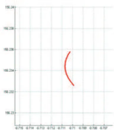
few of reflected rays pass through the camera lens, that is to say that not all rays are useful for the image formation. These ’successful’ rays (where PL is located in the lens) define a useful section of the caustic curve (Fig. 4).
In Fig.4-b, the virtual image of a source point is part of the caustic curve (the red part), Fig.4-a is simulated to compare with Fig.4-b.
Since the virtual image of a given source point is not a point but a curve, the corresponding image (going through the lens) is also a curve (Fig. 5, where the lens is supposed to be ideal), corresponding to the image of the catacaustic with the classical (ideal) lens transformation.
In Fig.5-a, all reflected rays (still) don’t intersect in a single point but (still) can be analyzed by the envelop (caustic) Fig.5-b (this curve is obtained from the previous equations and the ideal lens formula). This is another cause of blur in a catadioptric system. However, the real impact is very small as the red curve is also very small.
4.2 Image Formation from Multiple Source Points
The complete virtual image includes all source points, so the caustic has to be calculated for each of them. Actually, as seen previously, only the ’useful’ part of the caustic can be taken into account. To obtain the whole virtual image, the source point has to be moved everywhere.
We here consider a vertical line of source points to simulate all points of the scene (as the distance from the focus as almost no impact [12]) and corresponding caustics with the equations previously elaborated.
A simplified model is used here, which considers only one incident ray from the source point. The considered ray is the one for which the reflected ray reaches the center of the lens (pin-hole camera model). In other words, to one source
(a) Numerical simulation for real im-age
(b) Real image calculated with caus-tic equations
Fig. 5. Real image of a source point
point is associated only one point of the caustic. PH is the associated point on the hyperbola. Considering the SVP model, we can associate the equation of the incident ray (that goes from the source point to the first focus of the hyperbola) to the equation of the hyperbola:
yH xH = yS xS (11) (yH−c 2) 2 a2 − x2 H b2 = 1 (12)
Based on these two equations, we can obtain the coordinates of PH:
xH = ySc a2 xS − r 4y2 S a2x2 S + c2 a2 b2 − 4 b2 2y2 S a2 x2 S − 2 b2 (13) yH = yS xS · xH (14)
Even if the lens is not located at the second focus of hyperbola, i.e. not-SVP model, a similar method can be used to obtain the coordinates of PH (calculus are slightly more complicated but the principle is the same).
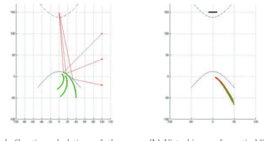
Fig. 6-a shows the three caustics issued from three source points of the vertical line. As we can see, the green curve has moved, and as a consequence the useful part (red points) has also moved. Obviously, outside the simplified model, the distribution of virtual image of a vertical line is not a simple curve but a curved surface.
(a) Caustics calculations of three source points
(b) Virtual image of a vertical line Fig. 6. Distribution of virtual image
Fig. 6-b shows, in green, the whole virtual image (i.e. the useful part of the caustics) of a vertical line and, in red, the points of the caustics considering the simplified model. As we can see, the simplified model is good enough to analyze properties of the catadioptric camera: depth of field, image formation, etc. 4.3 Comparison between the First Approximation and the Caustic
Approach
The caustic approach has two main advantages compared with the first approx-imation:
– For each source point, we can use only one incident ray to obtain the position of virtual point; this simplified model can help us to analyze the image for-mation of many complicated optical systems, e.g. multi-mirror catadioptric system.
– With the limit of the size of the lens, we can use caustic to get the the complete and accurate model of virtual image; this model can help us to analyze deeply the image formation of catadioptric system.
5
Applications
5.1 Depth of Field of a Catadioptric System
In our simulations, blur has appeared due to the use of cheap cameras (with a relative large aperture) and the compactness of our system (short distance between the camera and the mirror).
The depth of field of a standard camera depends on the focal distance, the aperture and the distance in the scene. A point is seen blurred if it is located
(a) Sharp zone around the mirror
(b) Sharp zone in the panoramic image Fig. 7. Sharp zone of a catadioptric camera
Fig. 8. Diameter of circle of confusion. x-axis represents the incident angle (o
), y-axis represents the size of the circle of confusion (mm).
outside the depth of field. In a catadioptric system, a point of the scene is seen blurred if its virtual image is located outside the depth of field of the camera.
The depth of field of a standard camera being defined between two planes, which are perpendicular to the optical axis, the depth of field of a panoramic camera is limited by two cones. Each cone is defined by a circle and the focus of the mirror. The circles are the intersection between the planes and the mirror (Fig. 7).
Let us suppose that the sensor is located at the incident angle of 0o(between the incident ray and the perpendicular plan), we can obtain the relation between the circle of confusion and the incident angle (Fig.8). The definition of blur is relative, it must also consider the image size, resolution, distance from the observer, etc. Our definition is that a point is blurred if and only if the associated circle of confusion is greater than two pixels. This allow us to quantify the depth of field of the catadioptric camera.
Let us note that the term of ’depth of field’ has a sense with a standard camera, as the sharpness is defined in the depth of the scene. Considering a
catadioptric camera, it would be more accurate to use the term of ’sharpness angle’, ’sharpness domain’ or ’sharpness zone’.
5.2 Mirror Choice
Our caustic-based model allow us to understand and anticipate blur in a cata-dioptric camera. Considering a given camera with its own parameters (that we cannot change) and the assembling constraints (usually due to the application), our model is used to determinate the best parameters of the mirror. ’Best’ mean-ing here that the sharpness domain is the biggest possible one.
In our case, using a USB webcam (focus=6mm, lens diameter=3mm, sensor size=4mm, resolution=640×480, pixel size is 0.005mm, and the distance mirror-camera is 150mm) in a robotics application, the best parameters for a hyperbolic mirror have been defined: a = 63.3866, b = 40.0892.
5.3 Image Resolution and Image Transformation
Moreover, the virtual image can be used to analyze the resolution of the space in the panoramic image, and, in the same time, to transform the panoramic image from the circular model to rectangle model without radial distortion (Fig. 9).
The correspondence between the incident angle and the pixel location is ob-tained according to the distribution of the virtual image; the curve is shown in Fig. 9-a. In Fig. 9-b, we use a series of circles to represent incident angles, from the outside to inside, the angles are −15o, −5o, −15o, −25o, −35o, −45o, −55o.
(a) Correspondence between angle (x-axis) and pixel location (y-axis)
(b) Spatial resolution in panoramic image
(c) Panoramic image in rectangle model Fig. 9. Relation between space and image
Based on Fig. 9-a, the transformation of a panoramic image to a rectangular image can be easily done in order to keep a constant radial resolution (Fig.9-c).
6
Conclusion
In this article, we describe an optical method to calculate caustics, and we present a new method to obtain virtual image, based on caustics. This new method is more complete, more accurate and easier to compute with respect to existing methods. Our model can be used in every cases, not only with the SVP con-straint in a catadioptric system. According to our model and the virtual image determination, we have defined several applications: the analysis of the catadiop-tric camera angle sharpness domain (’depth of field’), the determination of the best parameters of catadioptric system mirror to reduce the blur, and also the analysis of the relation between image and space. Since the caustic-based sim-plified model needs only one ray, it can be easily applied in more complicated optics system, e.g. multi-mirror catadioptric system.
References
1. Baker, S., Nayar, S.K.: A theory of single-viewpoint catadioptric image formation. International Journal of Computer Vision 35, 175–196 (1999)
2. Baker, S., Nayar, S.K.: Single viewpoint catadioptric cameras. In: Benosman, R., Kang, S.B. (eds.) Panoramic Vision: Sensors, Theory, Applications. Springer, Hei-delberg (2001)
3. Born, M., Wolf, E.: Principles of Optics: Electromagnetic Theory of Propagation, Interference and Diffraction of Light, 7th edn. Cambridge University Press, Cam-bridge (October 1999)
4. Bruce, J.W., Giblin, P.J., Gibson, C.G.: On caustics of plane curves. The American Mathematical Monthly 88(9), 651–667 (1981)
5. Hamilton, W.R.: Theory of systems of rays. Transactions of the Royal Irish Academy 16, 69–174 (1828)
6. Hecht, E., Zajac, A.: Optics. Addison-Wesley, Reading (1974)
7. Ieng, S.H., Benosman, R.: Les surfaces caustiques par la g´eom´etrie, application aux capteurs catadioptriques. Traitement du Signal, Num´ero sp´ecial Vision Omni-directionnelle 22(5) (2005)
8. Micusik, B., Pajdla, T.: Autocalibration & 3d reconstruction with non-central cata-dioptric cameras (2004)
9. Nye, J.: Natural Focusing and Fine Structure of Light: Caustics and Wave Dislo-cations, 1st edn. Taylor & Francis, Abington (January 1999)
10. Swaminathan, R., Grossberg, M., Nayar, S.K.: Caustics of catadioptric cameras. In: Proc. International Conference on Computer Vision, pp. 2–9 (2001)
11. Swaminathan, R., Grossberg, M.D., Nayar, S.K.: Non-single viewpoint catadioptric cameras: Geometry and analysis. International Journal of Computer Vision 66(3), 211–229 (2006)
12. Zhang, S., Zenou, E.: Optical approach of a hypercatadioptric system depth of field. In: 10th International Conference on Information Sciences, Signal Processing and their Applications (to appear 2010)