Time Resolved Two Dimensional X-Ray Densitometry of a Two Phase Flow Downstream of a Ventilated Cavity

Science Arts & Métiers (SAM)

is an open access repository that collects the work of Arts et Métiers Institute of Technology researchers and makes it freely available over the web where possible.

This is an author-deposited version published in: https://sam.ensam.eu

Handle ID: .http://hdl.handle.net/10985/8674

To cite this version :

Simo A MAKIHARJU, Céline GABILLET, Bu-Geun PAIK, Natasha A CHANG, Marc PERLIN, Steven L CECCIO - Time Resolved Two Dimensional X-Ray Densitometry of a Two Phase Flow Downstream of a Ventilated Cavity Experiments in fluids A Vol. 54, n°7, p.1561.11561.21 -2013

Time Resolved Two Dimensional X-Ray

Densitometry of a Two Phase Flow

Downstream of a Ventilated Cavity

Marc Perlin1 and Steven L. Ceccio1

1

University of Michigan, Ann Arbor, USA

2

Research Institute of the French Naval Academy - École Navale, France

3

Korea Institute of Ocean Science & Technology, Korea

4

Naval Surface Warfare Center - Carderock Division, USA

Corresponding author: Simo Mäkiharju, [email protected]

Abstract

To measure the void fraction distribution in gas-liquid flows, a two-dimensional x-ray densitometry system was developed. This system is capable of acquiring a two-dimensional projection with a 225 cm2 area of measurement through 21 cm of water. The images can be acquired at rates on the order of 1 kHz. Common sources of error in x-ray imaging, such as x-ray scatter, image distortion, veiling glare, and beam hardening were considered, and mitigated. The measured average void fraction was compared successfully to that of a phantom target and found to be within 1%. To evaluate the performance of the new system, the flow in and downstream of a ventilated nominally two-dimensional partial cavity was investigated and compared to measurements from dual tip fiber optical probes and high speed video. The measurements were found to have satisfactory agreement for void fractions above 5% of the selected void fraction measurement range.

Keywords: x-ray, densitometry, void fraction measurement, bubble probe, ventilated cavity, multiphase flow

Nomenclature

ai fraction of light scatter contributed by term i

bi measure of propagation distance of scattered light by term i

d bubble diameter (m) D the detected image E the un-degraded image

fe bubble probe sampling frequency (1/s)

H height of the backward facing step (127 mm) Fourier transform of h

h point spread function (1/m2)

I intensity of photon flux, number of photons per unit area and time (1/(m2s))

G greyscale value of light intensity (1) K Number of x-ray image frames

L length (m)

l12 streamwise distance between the optical probe’s tips (m)

lL latency length of the optical probe’s tips (m)

lc chord length of the gas measured by the upstream tip of the optical probe (m)

N total number of materials (1)

nb number of gas structures detected on the upstream tip of optical probe

Q injected air volume flow rate (m3/s) Qdet image intensifier detection efficiency

q non dimensional gas flow rate, Q/UHW (1) r radial distance (m)

Re Reynolds number, UL /

ν

t time (s)

ta transit time of a gas structure between the two tips of the optical probe (s)

taP most probable transit time of gas structures (s)

T measurement time of the bubble probe (s) U free stream velocity at the BFS (m/s) Ua gas velocity (m/s)

a

U statistical mean value of the gas velocity (m/s) UaP most probable velocity of the gas (m/s)

Uw water velocity (m/s)

W width of the model (209.6 mm) v bubble probe signal voltage (V) V photon energy (eV)

xn mass thickness of material, n (kg/m2)

x coordinate along the test surface , zero at the BFS (m) y coordinate normal to the test surface (m)

z spanwise coordinate (m)

Greek letters

α

δ

ρ density (kg/m3)

θ

σ

ν

µn/ρn mass attenuation coefficient of material n (m2/kg)

Subscripts a air i ,j number of term inj injection k frame number m mixture min minimum max maximum

n material designator (air, water, mix, etc.) OP optical probe

w water

0 initial

2 two-dimensional

Abbreviations

BFS backward facing step ESF edge spread function FFT fast Fourier transform II image intensifier LSF line spread function TTL transistor–transistor logic PSF point spread function RMSD root mean square deviation SNR signal to noise ratio

2D two-dimensional

1. Introduction

Gas-liquid and cavitating flows are encountered in many industrial and hydrodynamic applications, and it is often of considerable interest to understand the evolution and dynamics of the local volume fraction of gas or vapor. This is particularly important as we seek to develop physics-based models of the multiphase flows to predict the spatial and temporal evolution of the void fraction field. However, measurement of the local time-dependent void fraction has not always been possible, especially in higher speed flows where probes inserted into the bulk of the flow may perturb the flow considerably or where the flows are

optically opaque. Hence, it is desirable to develop measurement techniques that reveal the spatial distribution of the phase fractions without disturbing the flow.

In many applications, to measure the void fraction in a cavitating or other multiphase flow in a nonintrusive manner, electrical resistance and impedance techniques have been used quite successfully (Welle 1985; Ceccio and George 1996, George et al. 2000a; George et al. 2000b; York 2001; Holder 2005; Elbing et al. 2008). Impedance probes have been developed that are installed flush to a flow boundary or are inserted into the flow; also multiple boundary measurements of impedance can be used to deduce the impedance distribution within a domain (Cho et al. 2005). Combined with a model that relates the fluid phase topology (e.g. bubble, stratified) and the local impedance, the impedance field can be used to find the phase distribution. Impedance tomography systems have been developed successfully for gas-liquid, gas-solid, and three-phase flows, and a recent review is provided by Holder (2005). Impedance tomography systems can be constructed at relatively low cost, and can be designed to provide temporally resolved phase fields. The spatial resolution of such systems is limited by the finite size and hence number of electrodes that can be located on the domain boundary. And, most importantly for gas-liquid flows, the reconstruction of the impedance field is based on a “soft-field”, where the result is dependent on the flow topology and oftentimes an a priori knowledge of the phase distribution may be required to obtain a solution.

Conversely, radiation densitometry and tomography have the benefit of being a hard-field measurement, such that the beam path is not dependent on the distribution of the phases within the domain. Both gamma and x-ray sources have been used to examine multiphase flows, and several researchers have used x-ray imaging to investigate both cavitating flows (Stutz and Legoupil 2003, Coutier-Delogosha et al. 2007, Hassan et al. 2008, Aeschlimann et al. 2011) and bubbling fluidized beds (Hubers et al. 2005). A recent article by Heindel (2011) provides a comprehensive review of the use of x-ray systems in multiphase flow.

Presented here are the details of an x-ray densitometry system that has been developed to measure the volume fraction fields of nominally two-dimensional flows without the need for phase averaging. Our goal was to develop a system that would be appropriate for relatively high Reynolds number gas-liquid

and speeds to 10 m/s. For water flows, this would yield a Reynolds number on the order of 2 million. To resolve the dynamics of such a flow, the x-ray densitometry system would need to measure the phase fields at a minimum rate of 1000 frames per second.

As we intend to use the x-ray densitometry system to provide validation-quality data, we have attempted to characterize the most important sources of uncertainty associated with the measurement, and to account for their effect when possible. We then performed x-ray measurements on a two-dimensional cavity flow, and compared these measurements to those performed with optical probes and videography to further understand the advantages and limits of the densitometry system.

The manuscript is organized in the following manner. In Section 2 we summarize the basic x-ray densitometry technique and discuss some of its limitations and sources of uncertainty in our measurement of void fraction. In Section 3 we briefly discuss the optical probe measurement technique. In Section 4 we describe the partial cavity flow and the other associated measurement techniques. In Section 5 the measurements from the x-ray densitometry system are compared and contrasted with those from the bubble probes and high-speed videography. The conclusions are provided in Section 6.

2. The X-Ray Imaging System

2.1 Physical Principles

When a beam of high-energy x-ray photons encounters an object, a fraction of the photons passes through without scattering or absorption (attenuation). The fraction of attenuated photons depends on the object's mass attenuation coefficient, density and thickness. For a beam encountering a domain with N distinct materials, based on the Beer-Lambert law we can write

∑ = = −N n n n n x e I I ₁ 0 ρ µ (1)

where I0 is the original intensity of the photon beam at any given energy, I is the

the density, xn is the mass thickness ( ), and tn is the thickness over the

traversed beam path through material n. The attenuation coefficient is a function of material properties and photon energy, and is a known property for most common materials (Hubbell and Seltzer 2004). Based on equation 1, we can derive an equation relating the attenuation to the void fraction of a two-phase mixture (Stutz and Legoupil 2003, Hubers et al. 2005). A step-by-step derivation with the assumptions highlighted was provided also in Mäkiharju (2012). The void fraction,

α

_            = w a w m I I I I ln ln

α

where I signifies the intensities of photon fluxes that pass through a test section filled with a mixture, m, all water w, or all air a, at any one given photon energy, V. This relationship is valid for a monochromatic beam. But, as we shall discuss below, the x-ray source used is polychromatic, and hence use of equation 2 without full knowledge of In = In(V) introduces additional uncertainty.

2.2 Description of the X-Ray Imaging Setup

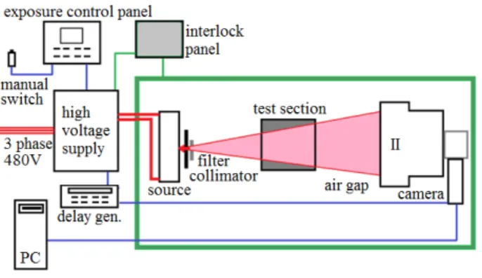
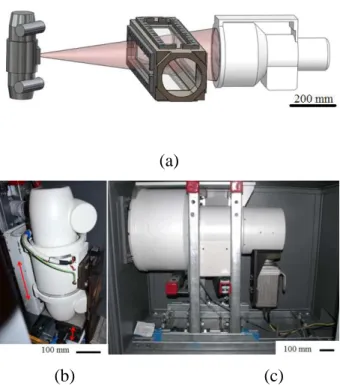
The components of the x-ray densitometry system are shown in figure 1. The operator sets the x-ray tube’s current, voltage, duration of exposure, and selects the image intensifier’s field size and attendant camera settings. Once an exposure is initiated, a signal is sent to the trigger unit (Stanford Research Systems model DG535 delay generator), which after a specified delay sends a TTL signal to the high-speed camera. Figure 2 shows the arrangement of the source, test section and imager, as well as the x-ray cone beam.

The x-ray photon flux needs to be sufficiently high, both in the number and energy of photons, to insure that a significant fraction passes through the domain. On the other hand, the energy must be low enough that sufficient attenuation occurs over short distances to yield an adequate contrast and signal-to-noise ratio when there are subtle differences in void fraction. Also, it was desired that the photon energy levels be suitable for use with commercial image intensifiers (II). The source selected is comprised of a Varian G-1092 insert in a Varian B-160H housing (figure 2b). This is a regular 150 kV rotating anode tube

800 mA (at 81kV) or 433 mA (at 150 kV), when supplied by the chosen 65 kW high frequency (100 kHz) generator with a high-speed starter (CMP 200 DR). The source had a selectable focal spot size of 0.6 or 1.2 mm, allowing less focal spot blur or higher power when using the smaller or larger spot size, respectively. The cone beam originating from the focal spot has a 24o included angle.

The imager subsystem (figure 2c) is comprised of a high-speed camera (Vision Research v9.0) coupled with a high efficiency, high-resolution II. A tri-field (30.5/22.9/15.2 cm diameter) II was chosen to enable image magnification without altering the physical setup of the experiment. For the current experiments the 22.9 cm input area was utilized. This II has a resolution of 48/54/62 line pairs per centimeter, conversion factor of 320 cdm2/mRs-1 and 65% detective quantum efficiency at 59 keV. An ordinary image intensifier was chosen, rather than an array of detectors, as an economical system that is still capable of rapidly acquiring information of the attenuation through multiple beam-paths (i.e. to acquire an instantaneous two-dimensional projection without phase averaging). After passing through the flow domain, the incoming x-ray photons enter the imager enclosure through a view-port, and interact with the II’s input phosphor to produce photons in the visible wave lengths that are then converted into electrons. These electrons are accelerated and incident on a second output phosphor. The output phosphor produces photons in the visible wavelengths detectable by an ordinary high-speed camera. The light collected at each of the camera’s 1.92 million pixels (or a subassembly of neighboring pixels) gives a measure of attenuation through one unique beam path. In the following subsection, we will discuss the characteristic of the systems, the most important sources of uncertainty, and the steps that can be taken to ameliorate them.

2.3 X-Ray Scatter

X-ray photons are scattered from matter in the beam’s path, and this can obscure the image details. To minimize this effect in medical applications, use is made of anti-scatter grids, and in some cases air gaps. In the current experiments, a collimator at the source and an air gap between the object and imager were used. The principle is to minimize the number of scattered x-rays reaching the imager; an air gap helps because the scattered photons tend to have large angles, different

from those of the primary beam's photons. The collimator is used to narrow the cone beam at the source, so that only the part of the beam illuminating the area of interest enters the domain.

2.4 Effect of Beam Hardening on the Measured Void Fraction

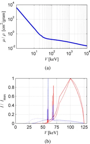
Except for monochromatic sources, an x-ray beam contains photons across a continuous spectrum of energies. Many detectors, including those used in the current research, do not resolve photon energy. The fraction of the beam that makes it through a domain varies with photon energy. As shown in figure 3a, the lower energy photons in the spectrum are attenuated preferentially compared to the higher energy photons (Hubbell and Seltzer 2004), leading to an increase in the average photon energy within the beam, denoted as beam hardening. Also, when using a polychromatic source and non-energy resolving detector, the value actually measured by the detector is the grey scale value of the detected light intensity, G, and not I, as defined in equation 2. The light intensity at each pixel of the camera is related to intensity I by

( ) ( )

_∫

where V is the photon energy, I(V) is number of photons of energy V incident on a given area of the imager screen and Qdet(V) is the image intensifier’s detection efficiency (the efficiency at which x-ray photons are transformed into photoelectrons and then into photons in the visible range). As both the attenuation and detection efficiency depend on the energy of the x-ray photons, V, I/I0 and

G/G0 are not equivalent and this can lead to an error in the measured void fraction, as we shall see next.

A polychromatic beam passing through material will always be hardened, and the low energy portion of the beam practically disappears, while a large fraction of the higher energy photons passes through the material. As will be shown in this section, it can be beneficial to always attenuate most of the lower energy photons, even when the domain has a high void fraction. We do this by “pre-hardening” the polychromatic beam by placing a filter between the source and object that we are imaging. For these experiments the beam was pre-hardened

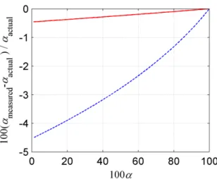
by a filter, which consisted of an ordinary carbon steel plate. To estimate the effect of beam hardening, the attenuation of the beams passing through the test section and two-phase domain was simulated. The x-ray source’s spectrum was estimated using the SpecCalc-software by Poludniowski et al. (2009). Figure 3b shows the simulated normalized photon energy spectra before and after the domain for cases with and without pre-hardening. Note that beam hardening modifies the shape of the spectrum of an x-ray beam as it passes through a domain, and lower energy photons in the spectrum are attenuated preferentially. However, the pre-hardened beam has a similar shape regardless of the void fraction. Consequently, the error arising from use of equation 2 with a polychromatic beam is modified and results presented in Figure 4. The error is dependent on the void fraction in the domain, but for all void fractions it can be seen that for the case simulated, pre-hardening reduces the potential error significantly. For example, at 50% void fraction the error with and without pre-hardening is 0.24% and 2.77% percent, respectively.

Alles and Mudde (2007) discuss the effects of beam hardening further and introduce “effective attenuation coefficients” for tomography. However, as shown in figure 4, for the cases discussed in this paper, the maximum bias error due to beam hardening can be reduced to less than 0.5% by simply pre-hardening. Thus this value is small compared to other sources of error and uncertainty discussed in the following sections. And, as the energy spectra were not measured to allow for empirical correction, pre-hardening alone was used to mitigate the effects of beam hardening in the current set of experiments.

2.5 Estimating Uncertainty of the Measured Void Fraction

To estimate uncertainty in the measured void fraction, we first considered that an 8-bit camera was utilized in the current setup. Therefore absence of light corresponds to a grey-scale value, G, of zero while the sensor saturates at a value of 255. To ensure that the sensor was never saturated, and that some light was reaching it, we chose the source settings with the aim of having the values of G at minimum and maximum void fractions be G ~10 and ~245, respectively. The actual values achieved were 6 and 240 for the example we will discuss. To obtain a reasonable estimate of the accuracy of the void fraction measurement (for a single pixel in a single frame), we assumed that each pixel of the camera was

correct to within ±∆G, where ∆G is the uncertainty in the intensity. Assuming that each variable of equation 2 is uncorrelated, the overall error in the resulting void fraction can be estimated as

.

(4)

Here the void fraction, , is based on equation 2. Assuming further that the uncertainty of intensity when measuring mixture, air or water is the same

( ) we can write

(5)

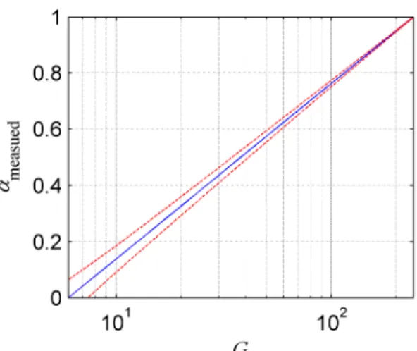
For the case of ∆G = ±1, for example, intensity with zero void fraction Gw = 6 and with void fraction of unity Ga = 240, we find the results presented in figure 5. This demonstrates that the error due to an incorrect grey scale value would increase exponentially as we go towards the low void fractions (corresponding to low G). That is, in both relative and absolute terms, the uncertainty is larger at lower void fractions.

The noise of the source, II and camera affects the spatial, temporal and void fraction resolutions. Presumably the noise is Gaussian and has zero bias, and therefore with a sufficiently large data sample the effect of noise would be mitigated after averaging. However, with short sample times, especially when imaging at 1 kHz, each of the camera’s pixels received light generated by a relatively small number of x-ray photons, making the random noise of the source also potentially significant. The signal to noise ratio (SNR) can be defined for each pixel as the ratio of its mean value and root mean square deviation, RMSD.

And, , where K is the number of frames (typically

~700) and G is the intensity at the pixel of interest. This SNR can vary depending on the flow condition, exposure and camera settings. In the region of interest in

was found to range from 22 to 62, with a 29 mean. A more comprehensive discussion of II noise is given by Bushberg et al. (2001).

The source intensity also had a slow drift, O(1%). According to the source’s manufacturer (Varian), the flux of photons from the x-ray source has time dependence caused by the generator, filament heating, anode heating, etc. For each set of images, the mean image intensity was plotted as a function of frame number. For all the void fraction calculations, data were considered only after the mean intensity was within ~0.5G of the final value. (If the recording was started before the intensity was within ~0.5G of its final value, or extended beyond the exposure time, the dataset was cropped accordingly.) Based on equation 5 the error caused by a 0.5G drift can be estimated as 2.6% and 0.2% at 10% and 90% void fractions, respectively.

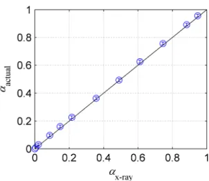
Thereafter, a direct validation and accuracy quantification of the void fraction measurement was conducted by placing a domain of known volume fraction in the beam path. Six containers with parallel walls spaced 1.6 mm to 101.6 mm apart were constructed as void fraction calibration “phantoms”. The baseline attenuation due to the test section and container material cancels, as can be seen when deriving equation 2. The combined path thickness of water was varied from 0 to 191.3 mm. The cumulative uncertainty of the water-path length through the six calibration volumes was estimated to be 1 to 2 mm, leading to a 0.5 to 1.0% uncertainty in the reference void fraction. Figure 6 shows the results from 14 different fill combinations with void fraction ranging from 0 to 1. The highest deviation, 0.0074, demonstrates the accuracy of the average void fraction measurement and is comprised likely of bias error due to container thickness; random variation of the source strength, I0; bias error varying with void fraction due to beam hardening; and the varying effect of ∆G as a function of the void fraction.

2.6 The Limiting Spatial Resolution

The resolution of the camera itself limits the highest detectable spatial frequency. Based on the Nyquist criterion the highest distinguishable spatial cyclic frequency, . In our case, is the linear dimension of a square area on the II's input plane, which is mapped onto a single pixel on the camera's

CMOS. The Vision Research Phantom V9.0 camera used has a 1632 by 1200 pixel CMOS. For the lenses used in the system, the image of the output phosphor is mapped onto a circle of diameter 1360 pixels. For the 305 / 229 / 152 mm (12 / 9 / 6 inch) selectable input sizes ∆ = 0.22 / 0.17 / 0.11 mm. Therefore, the camera alone limits the highest spatial frequency to 2.2, 3.0, and 4.5 mm-1 for the 305, 229 and 152 mm input fields, respectively.

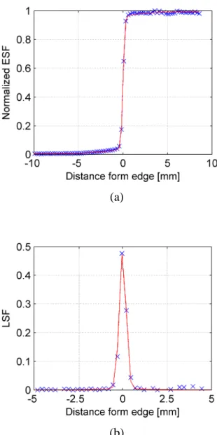
The spatial resolution of the entire system was quantified experimentally by two methods. First, a standard resolution test tool, with 0.63 to 1.97 lines/mm grids was used. The test tool was placed near the flow domain. The results indicated that in the basic system configuration we can resolve approximately 1.6 lines/mm. Secondly, the resolution was quantified based on the line-spread function (LSF) full width at half its maximum value. (The LSF is the in-plane derivative of the detected intensity variation normal to the image of a sharp edge (i.e. the derivative of the edge-spread function (ESF).) According to this definition, based on the data presented in figure 7 the spatial resolution is determined to be 0.46 mm. As expected (as the resolution is limited also by veiling glare, blur due to finite focal spot size and x-ray scatter), this is slightly larger than the resolution limit imposed by the camera alone, which was 0.33 mm.

2.7 Correction for Image Distortion

The x-ray image of any two-dimensional object placed in the cone beam’s path is distorted because the paths of the x-rays are not parallel over the domain (except possibly for a single beam path at a particular angle), and the image intensifier introduces distortion due to its geometry and the imperfections of its electric fields (Bushberg et al. 2001). Additionally, the camera optics can also distort the image of the II's output phosphor.

Correction for non-parallel beam path distortions was not feasible due to the noise in the signal and having only a single projection, i.e. having no redundant data (Mäkiharju 2012). Correcting for the remaining types of distortion is straightforward. Numerous researchers have proposed unwarping algorithms to correct for these distortions. For instance, Cerveri et al. (2002) discuss local unwarping polynomials and radial basis function neural networks. For our part, we used a calibration image and followed a procedure similar to that used in

Particle Imaging Velocimetry, except that the calibration grid was placed on the imager directly, and the markers had different attenuation than the surrounding material. We found that the de-warping functions in LaVision’s DaVis 7.2 provided an acceptable correction in the form of two-dimensional 3rd-order polynomials. Once found, the polynomials were implemented in a Matlab code and used to de-warp all the images. Figure 8 shows an aluminum calibration grid that was placed on the II-screen, as well as the unmodified and de-warped x-ray image of the calibration target. As is evident in figure 8c, the distortion correction was successful.

2.8 Correction for Veiling Glare

Veiling glare tends to smooth sharp interfaces between different volume fractions and it is particularly obvious, and detrimental to image quality, when high intensity and low intensity regions are nearby in the same image. This occurs in regions of strong void fraction gradient, such as free surfaces. Veiling glare is related to photon scatter within the imager system. Significant scattering can occur in the II’s output phosphor (Seibert et al. 1984), although the scattering of photons and electrons in the input screens, and the scattering of visible wavelength photons in the camera's lenses can also contribute.

The image recorded by the camera can be treated as a convolution of the un-degraded image with the point spread function (PSF) of the imager. Thus, correction for veiling glare can be attempted using deconvolution as in Seibert et al. (1984, 1985 and 1988), and we can write

(6)

where D is the detected image, h is the PSF, ** signifies a 2D convolution and E is the un-degraded image we wish to recover. In the frequency domain this can be written as a multiplication

Here F2[A] denotes the two-dimensional Fourier transform of any variable A. We solve for E by dividing through by the Fourier transform of h and performing the inverse Fourier transform , yielding

(8)

Seibert et al. (1985) proceed by analytically transforming h to obtain its Fourier transform’s reciprocal, . Alternatively, we can employ a known or assumed PSF with common deconvolution algorithms. In the present work we employed Matlab’s built-in function, “deconvlucy”, based on the Lucy-Richardson method.

To correct the image, several possible point spread functions are discussed by numerous authors including Seibert et al. (1984), Smith (2006) and Poludniowski et al. (2011). The last reference provides a very general form of PSF, from which most proposed PSFs can be extracted:

(9)

Here a1, a2 and a3 are coefficients that can be thought to be related to the fraction of light scattered by various processes (represented by the different terms), r is the radial distance, b's can be considered to relate to mean propagation distances of scattered light, and is the Dirac delta function of r.

The ESF is straightforward to measure, and for that reason it was used to estimate the PSF. For the current data we used the relationships between ESF and PSF given in Johnson (1973). Therefore the ESF given by

where x here is the coordinate normal to the edge, is related to the point spread function

(11)

Again, a1 and a2 are coefficients that relate the fraction of light scattered by various processes. However, we will simply treat these as empirical fit parameters. As seen in figure 7a, a least squares approximation of equation 10 matched the data well with coefficients a1 = 0.08811, a2 = 0.91189, b1= 1.722 mm and b2 = 0.244 mm. With these coefficients, equation 11 was used to correct for the veiling glare in the cavity closure region. To avoid high frequency oscillations, the term with the lower value of b was set to zero for the deconvolution, as done by Poludniowski et al. (2011). The effect of this correction is seen in figure 12d.

2.9 The Limiting Temporal Resolution

The temporal resolution of the x-ray based void fraction measurements is limited by the camera’s frame rate, number of photons available to record data with sufficiently high SNR and by the imaging system’s response time. The imaging system’s response time is set by the finite rise and decay times of the II's phosphor. The data sheet for a nominally identical image intensifier (Thales 2006) lists that for a 5 mR/s exposure, the luminescence rises to 50% and 80% of the final value in 1 ms and 10 ms, respectively. The reported decay times are 1 ms and 10 ms to decay to 30% and 10%, respectively. Thus, the decay rate will not conform to a single time constant, , fitting . However, based on the 10 ms luminosities alone, the rise and decay time constants would be 6.2 ms and 4.3 ms, respectively.

We attempted to quantify the imagers response time by two methods. First, the response time was based on the measured variation of light intensity at the beginning and end of exposure, and assuming the source's rise and decay times to be orders of magnitude faster (so that any lag in the rise of intensity would be due to the phosphor). This approach suggested that the imager's time constant would be ms. The second approach was to place a metallic disk spinning at 386

rpm in front of the source. The disk had a 6.4 mm hole located 28.1 mm from the center of rotation. By recording an x-ray movie at 1000 fps of the spinning disk and plotting the time trace of mean intensity over a 10 by 10 pixel region, it was found that the intensity at a given location reaches 32%, 63% and 90% of the final value within 1, 2, and 9 ms, respectively.

While the phosphor’s decay time constant is O(3ms), differences over shorter time periods are clearly detectable, and for similar imagers O(10 kHz) frame rates have been used successfully (e.g. Aechlimann et al. 2011). Therefore, for the current experiments, where data were acquired to 1 kHz, it is postulated that changes over 1 ms time scales can be reliably detected and the information used, as long as the limitations of the system are understood. In the current work our highest flow speed was 1.8 m/s, and hence a bubble could move 1.8 mm in the 1 ms interval between frames. While some ghosting was certainly present, it was not readily observable in the data.

2.10 The X-Ray Image Processing Procedure

To process the data while satisfying the previously discussed criteria and optionally accounting for veiling glare, when its effect was significant, the following procedure was adopted. First, each movie was processed to produce a time trace of frame-averaged image intensity, which then was used to register when the recording was initiated compared to the time that the source was energized. Then, a range of frames was defined wherein the average image intensity was nominally constant. Within this range, all frames were averaged to obtain the average intensity for each pixel for the all air Ga, all water Gw and mixture Gm conditions. Second, each image was corrected for geometric distortions and the data were mapped onto a new image where, depending on the spatial averaging chosen, each new larger pixel had an average intensity based on that of 4 to 100 of the original pixels. Third, and the optional step, a veiling glare correction was applied via Lucy-Richardson deconvolution with 10 iterations. Fourth, the void fraction at each pixel of each frame was calculated based on equation 2, with the physical constraints limiting the results such that α(t,x,y) = 0 if Gm(t,x,y) < Gw and α(t,x,y) = 1 if Gm(t,x,y) > Ga, which occasionally occurred

due to statistical variation and light scatter. These corrected images were deemed the x-ray results.

3. Optical Bubble Probes

A dual fiber optical probe and an optoelectronic module made by RBI-Instrumentation were used to measure the void fraction and the streamwise gas velocity, Ua as well as the bubble size distributions. The optoelectronic module

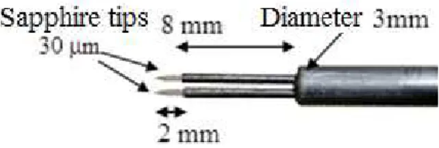
was used to inject light into the fibers of the probe, detect the reflected signal and convert it into a voltage level. Each optical fiber pointed end has a cone shaped tip that is used to detect reflection when the tip is immersed into the gas, whereas there is only refraction when the tip is immersed into the liquid. The probe consisted of two 30 micron sapphire tips, separated in the streamwise direction by distance l12 that was 1.05 mm (figure 9).

In order to have a good detection of a gaz structure pierced by the tip, the gas residence time on the tip must be larger than the response time of dewetting-rewetting process The resolution of the tipsis then limited by the response time of the tips during the de-wetting process (response time of the rewetting process being much shorter).. As shown in Cartelier (1990), above a critical velocity around 0.2m/s, the response time of the dewetting process is expected to evolve as the inverse ratio of the gas interface velocity. Thus, the product between the response time of dewetting and the interface velocity remains constant, it is called the latency length, which is representative of the size of the smallest gas structure that can be detected by the probe’s tips with a good resolution. The latency length lL has been characterized experimentally for a static interface with no curvature,

following a procedure detailed in Cartelier (1990). For the probe’s tips used, itis 0.50 mm.

3.1 Optical Probe Data Processing

When the photo detector signal voltage was greater than a prescribed threshold, the gas characteristic function was set to 1; otherwise it is set to 0. The void fraction was based on the time average of the characteristic function of the tip. The time corresponding to the maximum value of the cross-correlation function (based on the two gas characteristic functions of the probe tips) was representative of the most probable transit time of the gas between the two tips,

taP. The transit time is defined as the time difference between the times indicating

the beginning of the gas structure detection on each tip. Thus, a most probable gas velocity was obtained as U_aP=l₁₂ t_aP. The signal from a transient gas structure was recognized as an associated gas structure if the signals from the two tips had a time delay (corresponding to transit time) that was within a time-window around the most probable transit time, taP. The velocity of different associated gas

structures Ua was deduced based on l12 and the transit time.

The mean velocity Ua _{and its RMSD value were deduced by weighting the}

velocity of each associated gas structure by its residence time measured on the upstream tip. The determination of the velocity distribution by this method is well suited for unidirectional flow (reverse or not),but it is not appropriate for the flow of high void fraction (> 90%). Indeed, for high void fraction in the air cavity or air layer, it was difficult to extract a most probable transit time from the cross-correlation function.

In general, when a gas bubble is pierced by the tip, the bubble center doesn’t cross the tip. Thus, the bubble is not expected to intersect the tip along its diameter but along a shorter length, that is called the chord length. The chord length lc of each associated gas structure (bubble) was obtained as the product of its velocity and its residence time on the upstream tip (upstream is relative to the local direction of the flow). This made it possible to determine the bubble chord length distribution.

When the probe was immersed in a bubbly flow, the inverse method developed by Clark and Turton (1988) was used to determine the bubble size distribution. This method was applied successfully in Gabillet et al. (2002), for the case of bubble injection along a wall for bubbles O(1 mm) and void fraction less than 30%. This method is based on joint probability density functions that give the likelihood of having a chord length for a given bubble size. It requires an assumption on the bubble shape (eccentricity). It also assumes that the largest chord length detected is equal to the largest bubble major axis diameter to be found in the bubble size distribution. Assumptions of both spherical and ellipsoidal bubbles, with varying eccentricity ratios, were tested.

3.2 Uncertainties of the Measurement

These measurements are sensitive to the voltage threshold levels applied when building the characteristic function. If vmin and vmax are the voltage levels obtained in the liquid and gas respectively, then varying the voltage threshold level in the range [vmin, vmin + (vmax-vmin)] leads to a significant variation of the measured void fraction value that can be modeled by equation 12. In this relation it is assumed that the error in the residence time determination is the same for each gas structure and is equal to the time of the de-wetting process of the tip (i.e. lL/Ua). This leads to an error in the void fraction determination representative of

the ratio between the latency length and the chord length of the gas structures:

∆

α

α













≈ ±

n

l

2

α

TU

≈ ±

l

2

l

.

Assuming that the voltage difference in the gas and liquid is the same for the two tips and that the gas structure is pierced by the two tips in the same way, the uncertainty in the velocity measurement due to the threshold level is a systematic error that compensates if the two tips have the same latency length and yields

∆U_a U_a      = ± lL1−lL2 2l₁₂

.

The uncertainty in the chord length determination results from the combination of errors in void fraction and gas velocity determination given by

∆

l

l













= ∆

U

U













+ ∆

α

α











.

In addition we can write the uncertainties in void fraction and velocity linked to the sampling frequency as

e b f T n

α

α

α

where nb is the bubble number and T is the measurement time.

The relative uncertainty in the determination of void fraction and chord length due to the sensitivity to the voltage threshold level was estimated based on equations 12 and 14. It was less than ±20% and it was decreasing (relative uncertainty less than 5%) for high void fraction (α > 30%) associated with longer

residence time. Assuming that the error in the determination of the residence time is maximal, note that this uncertainty is overestimated For the gas velocity, the sensitivity to the threshold value in the range [vmin + 0.30(vmax-vmin), vmin + 0.70(vmax-vmin)] was examined. Regardless of the void fraction value, the relative uncertainty due to the voltage threshold was less than ±3% for the gas velocity determination.

The transit time-window, used to associate gas structures of the two tips, was chosen so as to have a velocity distribution centered on UaP =

1−

β

(

)

(

β

)

 . A value of

β

to 50 kHz. Based on equations 14, 15 and 16, this sampling frequency leads to a possible relative error of ±5%, ±6%, ±11% for the determination of the void fraction gas velocity and chord length, respectively.

The measurement time required depended on the void fraction. However, for all flow conditions considered it was 30 seconds or 60 seconds to have at least 300 gas structures detected on each tip near the wall. The convergence of the data as a function of the number of associated gas structures was examined, and for 100 associated gas structures the mean value of the velocity was accurate to within 2% (with 68% confidence level).

Repeatability between the different experiments was also explored. The RMSD value was less than 20% of the mean value for the void fraction, and less than 5% of the mean value for the velocity. RMSD values of the void fraction were higher at the edge of the cavity when it was filled with air. The RMSD value of the mean velocity was larger further from the wall where there was a change in the sign of the velocity (edge of the reverse flow). To compensate for errors of reproducibility, the void fraction and the mean velocity were averaged among several runs (between 3 and 8 runs).

The optical probes were attached to a traverse mechanism described in Mäkiharju (2012). The traverse enabled the probes to be positioned with accuracy of at least 0.2 mm. However, the absolute position relative to the model was only accurate to within ±0.7 mm, as the tips could not be allowed to touch the model

the model and probes installed. For each flow condition investigated, the accuracy of the void fraction and velocity measured by the probes is indicated by error bars included in the first plot containing the data.

4. The Partial Cavity Flow

4.1 The Recirculating Water Channel

The x-ray system was designed for use with an existing cavitation tunnel at the University of Michigan. However, a new test section, 864 mm long with a (209.6 mm)2 cross-section and 28.6 mm chamfer in the corners, was constructed for these experiments. Test section windows 152 mm by 864 mm were used to provide good optical access. The windows were made as thin as 1 cm, to reduce the baseline x-ray attenuation. In the empty test section the flow can achieve speeds in excess of 18 m/s, while the pressure can be varied from that below vapor pressure to over 200 kPa. Additional details of the flow facility are provided by Oweis et al. (2004).

4.2 The Test Model and Flow Conditions

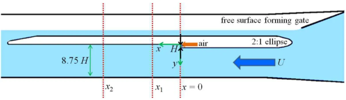
The test model was a flat plate that spanned the width of the test section, W = 209.6 mm, and had an overall length of L = 910 mm. The model had a backward facing step of height H = 12.7 mm and was located 350 mm from the leading edge. The boundary layer upstream of the cavity separation was tripped at the leading edge of the 2:1 ellipse. Air was injected from the base of the step through a 4.7 mm tall slot spanning the width of the model. The plate thickness downstream of the step was 19.1 mm. The air was introduced first into a chamber inside the model, and exited the chamber through a porous plate to produce a spanwise uniform flow. The spanwise uniformity of the air injection was measured using a hot wire anemometer, and was found to be uniform within the accuracy of the measurement. An upstream gate was used to form a free surface above the model, enabling air removal during long periods of air injection. Figure 10 shows a schematic diagram of the model and free surface-forming gate in the test section.

The free stream speed for each condition was measured via a Pitot tube placed in the flow at the spanwise centerline with its tip 17H upstream of the

backward facing step and ~ 2H from the step’s surface, with the pressure difference measured with an Omega Engineering PX2300-5DI, 0 to 5 psi differential pressure transducer. The free-stream flow velocity, defined as the bulk flow speed at the position of flow separation above the backward facing step, was U = 1.80 ± 0.05 m/s for all data discussed in this paper. The pressure in the test section was kept nominally at 1 atm via vents to the atmosphere. The transducers were connected to a National Instruments DAQ NI USB-6259, and signal processing and recording were performed using Labview 2009 Virtual Instruments. The injected gas flow rate, Q, was measured with two flow meters. For flow rates to 7.97 x 10-6 m3/s the flow meter used was the Omega Engineering FL-2001 with manufacturer specified accuracy of ± 0.39 x 10-6 m3/s. For flow rates above 7.97 x 10-6 to 3.93 x 10-5 m3/s the flow meter used was Omega Engineering FL-2003 with manufacturer specified accuracy of ± 0.20 x 10-5 m3/s. The water was filtered tap water, and its temperature was maintained at 25.0 ± 1 o

C, except for the high-speed video that was recorded previously when the water temperature was 18.0 oC.

High-speed video of the flow was recorded using a Vision Research Phantom v710 camera and two Arri-studio lights. However, only at the lowest air fluxes were the individual bubbles distinguishable (i.e. minimal overlap when viewed from below). Several hundred independent frames were processed manually, to obtain the bubble size, minor-to-major axis ratio, and velocity histograms. Assuming that the bubble edge location was measured correctly within ± 1 pixel, the diameter measurement is accurate within ± 0.12 to 0.2 mm. The usual displacement over the time differential was greater than 50 pixels, thus the velocity can be assumed accurate within ± 0.04 m/s. In total 1236 bubbles were measured. Also, the void fraction, as a function of distance from the test surface, could be estimated as the depth of field was known and the flow was assumed to be nominally two-dimensional.

4.3 The Single Phase Flow in the Vicinity of the Backward Facing Step

To characterize the inlet boundary conditions, the turbulent boundary layer upstream of the backward facing step near the location of flow separation was

comprised of a LaVision FlowMaster 3s camera, New Wave Gemini 200 lasers, external LaVision PTU 9 timing unit and a PC running LaVision's DaVis 7.2. At the flow speed of 1.8 m/s, the boundary layer upstream of the step was turbulent and conformed to a 1/7th-velocity profile with thickness

δ

θ

Additionally, the single-phase flow downstream of the backward facing step was measured. The length of the single-phase separation bubble was found to be approximately 6.5 H, which is consistent with the historical value for the case of a low expansion ratio, 1.13 in this case (Adams and Johnston, 1988).

4.4 X-Ray, Optical Probe and Video Measurement Locations

Measurements of the cavity flow were collected in two distinct flow regions. The first region was between 0 < x / H < ~ 7, which corresponded to the closure region of the partial cavity. Here x is the stream-wise distance from the step and H is the step height. The second region beyond x/ H = 8 corresponded to the bubbly flow in the cavity wake. The x-ray images were acquired with three different fields of view that extended from -1.5 < x / H < 9, 1 < x/ H < 11.5 and 11 < x/ H < 21. The optical probe measurement locations are indicated in figure 10 and were x / H = 5 and x / H = 21. The high-speed video was recorded for 10 < x / H < 19.

5. Results

5.1 Partial Cavity Flow

Figure 11 shows two images of the partial ventilated cavity. Figure 11a is an oblique view from below, figure 11b is an elevation view of the cavity for U = 1.8 m/s and Q = 2.2 x 10-5 m3/s. Therefore the non-dimensional gas flux, q = Q / UHW = 4.6 x10-3. The free surface detached cleanly from the apex of the backward facing step, and a nominally two-dimensional gas cavity formed downstream. The gas cavity closure occurred at x / H = 6.5 ± 0.5, which compares well with the location of the single-phase cavity closure of x / H ~ 6.5 (Adams and Johnston 1988). Additionally, the interface of the cavity had small waves associated with the ingestion of the turbulent boundary layer upstream of the cavity closure.

The cavity closure was nominally two-dimensional. The gas was entrained into the cavity wake as ligaments of gas that were stretched and then divided into bubbles. Some of the bubbles were advected immediately downstream, while others briefly remained in the recirculating flow region of the cavity closure. This resulted in a bubbly flow, with thickness on the order of the cavity thickness, advected from the cavity closure.

5.2 Cavity Closure Region

Figure 11 shows the cavity near the backward facing step for q = 4.6 x10-3. The void fraction was essentially 100% within the cavity upstream of x / H ~ 3, but due to multiple scattering (reflection and refraction) it could not be estimated in the closure region based on visible light images alone, which is a problem similar to those in many cavitating flows. Hence, the x-ray system was used to measure the void fraction in the closure region, and the results are presented in the following.

Figure 12a shows a raw false color (i.e. a colored 8-bit grey-scale image) x-ray image of the partial cavity. This 8-bit representation of light intensity is related to attenuation of the x-ray beam and hence yields a quantitative measure of the void fraction. Figure 12b shows the void fraction distribution, and near the bottom of the cavity where we had a sharp 100 to 0% void fraction change; the effect of veiling glare can be seen clearly. Figure 12c exhibits the image corrected for veiling glare. Although little change was evident, the affect can be clearly seen in figure 12d that compares the uncorrected and corrected distribution at x / H = 2.5. The veiling glare correction is imperfect, and some smearing of the interface persists due to the non-parallel beam paths, but the post-processed image is improved. The 2D projection of the void fraction distribution revealed the existence of strong gradients in the cavity closure region. Figure 13 shows the local profile of void fraction perpendicular to the flow boundary, y / H, at different stream-wise locations, x / H, for q = 1.64 x10-3, q = 4.60 x10-3 and q = 8.21 x10-3.

To obtain data for comparison to the x-ray measurements, an optical probe was placed in the closure region at x/ H = 5. Figure 14 presents the measurement of local void fraction and mean gas interface velocity based on the dual tip optical

4.60 x10-3 and q = 8.21 x10-3. We observe that the tip upstream of the local flow always recorded a higher void fraction, as the second tip was in the wake of the first and some bubbles could be deflected from the probe. (Indeed, the downstream probe detects 10% fewer gas structures than the upstream probe, in agreement with deflection by the tip located upstream.) More deflection was encountered at the edge of the recirculating region (20%) where the stream-wise velocity was weak. Note the large error bar for the void fraction in this particular region (figure 14b at y / H ~0.35). This was due to the uncertainty in the void fraction determination when applying the voltage threshold level (eq. 12). This uncertainty was increasing a lot for low velocity at the edge of the recirculating region.These data are compared to x-ray data in Section 5.4.

Figure 14d shows the velocity profiles in the closure region of the cavity, which align well for q = 4.60 x 10-3 and q = 8.21 x10-3. For q = 4.6 x 10-3, the velocity profile exhibits clearly the recirculation in the near wall region of the cavity. The edge of the recirculating region was associated with a local increase in the void fraction. For the maximum air flow rate, the cavity was completely filled with air (α∼100%) and thus the algorithm would not be able to associate the gas structures on the two tips. Hence, the velocity was not plotted for y / H < 0.7.

Figures 15 a and b exhibit the bubble size and velocity histograms, respectively. These data are for q = 4.60 x10-3 at x/ H = 5, and y / H=0.615. The mean bubble diameter was 1.92 ± 0.07 mm (RMSD value). The number of bins for the bubble size histogram determination is limited by the inverse method that can lead to empty classes or negative values of the probability function if the number of associate bubbles is too small. The smallest detected bubbles approached the limit of what is detectable with the optical probe (~0.5 mm). The vast majority of the bubbles were O(1mm) and these were not individually detectable by the current x-ray system; however, their cumulative contribution will significantly affect the x-ray attenuation.

5.3 Bubbly Flow in the Cavity Wake Region

In the wake region with the lowest gas flux it was possible to measure the bubble velocity and size distributions directly from video of the flow, and this could be compared against the optical probe data. Figure 16a shows a photograph of the bottom view and 16b a photo of the side view. All results from the

high-speed video are for 1.8 m/s high-speeds with ventilation rate q = 1.64 x10-3. We note that the Weber number, , based on the bubble major axis and nominal free stream speed of 1.8 m/s would be O(100), for a typical 2 mm diameter bubble, and hence many of the bubbles are likely to be ellipsoidal, as evident in figure 16b. To demonstrate this more clearly, figure 17 shows the eccentricity ratio histogram from the video, and also compares the bubble size, and velocity histograms to the ones obtained by the optical probes. Obviously figure 17a shows that the bubbles were predominantly ellipsoidal. In figure 17b we can see that only the largest bubbles are individually detectable from single x-ray frames. (While the smallest bubbles are not individually resolvable from unsteady data, these more numerous smaller bubbles contributed to the overall time averaged void fraction measured via x-ray.) For the optical probe data, different models of eccentricity were tested, based on the eccentricity ratio that is available from the video recording.

Figure 17b shows histograms based on three different assumed eccentricity ratios. The mean actual eccentricity ratio was around 1.31. Implementation in the inverse method of different values for the eccentricity ratio (1, 1.31 and a fit as a function of the major axis) lead to very similar bubble major axis histograms measured by the optical probe, as shown by figure 17b. The mean bubble size based on video and optical probe data were 1.86 mm and 2.26 mm respectively. The mean velocity, Ua /U, based on video and optical probe data were 0.64 and 0.68, respectively. The bubble size and velocity histograms show a small difference in the bubble populations based on video and based on optical probe data. Also, the bubble population based on optical probe data was not affected strongly by the assumed bubble eccentricity used in the data processing.

The void fraction in the wake was on the order of 1%, and thus for these measurements the x-ray source settings were adjusted to achieve improved contrast, as it was possible to use higher beam intensity without saturating the imager. A 12.7 mm container fixed between the source and the object could be filled and emptied to obtain reference intensities Ga and Gw, where 100% void fraction was defined as when the test section was full and the container empty. The container was then maintained full during data acquisition. Figure 18 shows the void fraction distribution based on x-ray measurement for q = 1.64 x10-3 and q

becomes more significant, the stream-wise evolution of the void fraction distribution is evident. To ensure that the x-ray provided reliable data in this challenging low void fraction flow, the dual fiber optical probe data were used for comparison. Figure 19 shows the local void fraction and mean gas velocity profiles obtained by the optical probe at x / H = 21. By comparison to the cavity closure region, the air layer at the highest gas flux became thinner, whereas the bubbly layer at the smaller gas fluxes extends further. While the void fraction data can be compared directly to that obtained by x-ray, the velocity information can be used to calculate the total gas volume flow rate based on void fraction measurements from both techniques. This can then be compared to the injected gas flow rate measured by the rotameters.

5.4 Comparison of the X-Ray, Optical Probe, and Video Measurements

The void fractions measured with the x-ray system and by the optical probe at x / H = 5 are compared in Figure 20. The same behaviors are clearly observable, as the distributions peak near y / H ~ 0.2 and exhibit a near plateau around y / H ~ 0.5. However, the data do not match; in fact any small deviation in flow conditions or measurement location mismatch would have a large effect due to the rapid streamwise evolution seen in figure 13b. The x-ray measurement is also effected by the imperfectly corrected veiling glare, non-parallel beam paths, and signal noise. For the optical probe data, it should be noted that the presence of the probe itself can perturb the flow, especially where reverse flow occurs such that the probe is influenced by its own wake. A reverse flow can be seen in figure 14d, and data in figure 14b could be affected by the flow perturbation caused by the probe. In this same figure, the effect of the local flow direction is clear, the measurement performed by the probe upstream relative to the local direction of the flow is more representative of the void fraction. Indeed, the probe downstream always records a lower void fraction, this is caused by some of the bubbles being deflected in the wake of the upstream probe. The probe can induce deformation of the bubbles, local deceleration, and bubble deflection (bubbles avoiding the tips, including the upstream tip relative to the local direction of the flow). Julia et al. (2005) has characterized the contribution of these different effects to the void fraction measurement for bubble diameter between 3 and 5 mm

and for flow velocity between 0.22 and 0.28 m/s. For these flow conditions, they highlighted that deflection and deceleration effects compensate for each other. The deformation effect is the most prominent and can lead to an underestimation of the void fraction by as much as 50% of the local void fraction value.

Figures 21 a and b show a comparison of the average void fraction profiles obtained by optical probes, x-ray and video (only in 21a) at x / H = 21. For the video data, the number of bubbles was insufficient for convergence, as random fluctuations in the distribution are apparent. Given the increasing uncertainty of the measurement at the low void fractions, scatter, limited averaging time of the x-ray dataset used, veiling glare, non-parallel beam paths, etc. the agreement is quite satisfactory. Also, due to the stream-wise-evolving void fraction profiles, any positional uncertainty of the x-ray compared to the optical probe will contribute to a difference between the profiles. As seen in figure 18 we observed that the void fraction profile in this region is still evolving, but much less dramatically than in the cavity closure region.

The comparisons to optical probes, issues related to veiling glare and non-parallel beam paths are discussed in more detail in Mäkiharju (2012), but these data illustrate a measure of the capability of the system used in this study. With the x-ray measurements it is possible to quantitatively describe and to gain new insight into the physics of the fluctuations, cavity breakup and bubble shedding at various flow conditions.

Finally, table 1 presents the injected gas flow rate compared to that calculated based on optical probe and x-ray data assuming fully 2D flow. Figure 19d had showed the velocity as a function of distance y / H, as measured by the dual tip optical probe. Knowing the velocity profile and using the optical probe and x-ray densitometry void fraction data, the gas volume flow rates are calculated from

. ₍₁₇₎

Here W is the span of the model, 209.6 mm, is the measurement location spacing normal to the model surface, u(y) is the flow speed parallel to the model surface measured by the optical probe and is the local void fraction. (The

upstream measurement location was within the complex recirculation region where the presence of the optical probe more likely affected the flow, and hence a similar comparison was not attempted for data from that position.)

In table 1 we observe that the volume flow rate was overestimated at the lowest gas flux, especially by the x-ray. The reason for this overestimate can be understood readily by revisiting the void fraction distributions presented in figure 21. Therein we see that the void fraction is overestimated at values below 0.4%. Besides the possible effect of short averaging times and veiling glare of the x-ray images, at these low void fractions the calculated value is extremely sensitive to the smallest error in any of the light energies as can be seen from equation 4. However, as the gas flux is increased, the relative uncertainty is reduced, and the gas flux calculated from the x-ray data moves closer to the injected value.

6. CONCLUSIONS

We have demonstrated how time-resolved x-ray densitometry can be successfully used to measure the volume fraction fields for nominally two-dimensional flows, and this system was demonstrated on a canonical flow: a cavity forming at the base of a backward facing step and the bubbly flow in its wake. The current system described here can quantitatively measure the time-averaged two-dimensional projections of 0 to 100% void fraction to within 2%, distinguishing features of O(1 mm), and detecting changes at time scales on the order of 1 ms through an enclosed domain of a gas/water mixture that is ~ 21 cm thick.

Video and optical probe measurements were compared to the x-ray data. The agreement between measurements of volume fraction using the optical probe and x-ray data yielded satisfactory agreement within understood levels of uncertainty. In particular, this was the case for unidirectional flow at x / H = 21, where the optical probe perturbs the flow the least and where the void fraction was above 0.5%, conditions that are optimal for each measurement method. In this case, the void fraction profiles measured using the x-ray system showed the best agreement with those obtained with the optical probes. The gas volume flux derived from video, bubble probe, and x-ray data compared well with the known amount of injected gas.

We note that the x-ray acquired data quite rapidly in comparison to the point probes. To acquire the void fraction profiles shown in figures 14 and 19 using the optical probes required two hours for each condition. The x-ray data required only a few seconds per condition and also provided information on the stream-wise evolution of the void fraction. Given that the x-ray had better than 1 mm spatial resolution, using any point probe (such as the optical probe) would require more than eight days of continuous operation to acquire the same spatial distribution (assuming three minutes per point covering an area 30 mm x 140 mm, with points every 1 mm).

The x-ray system was able to measure the volume fraction in the recirculating cavity closure region, where the void fraction had strong spatial gradients. The non-unidirectional flow and strong gradients make the use of bubble point-probes problematic. But, x-ray measurement is not affected by this, and also the flow is not perturbed. However, any x-ray data acquired with a system such as ours will often have non-negligible veiling glare. It should be taken into account when interpreting the data and, as shown, it can be at least partially mitigated by deconvolution. The densitometry measurements revealed the spatial evolution of the time-averaged and fluctuating void fraction distribution in the cavity closure, and it was seen that even at x / H = 21 downstream of the backward facing step, the void fraction distribution was evolving in the streamwise direction, and on-average the bubbles were migrating closer to the surface. It was also possible to observe the motion of the cavity closure as well as some of the largest individual bubbles in the wake region with the x-ray system. However, the spatial resolution of the x-ray system was not sufficient to resolve images of most individual bubbles, which were below 5 mm in diameter in the instantaneous frames.

Acknowledgements

We acknowledge the assistance of Prof. Michael Flynn and Dr. Alexander Mychkovsky during the design of the x-ray densitometry system, and Mr. Christopher Haddad for his contribution in processing of the high-speed video images. The authors are grateful for the support of the Office of Naval Research under grant N00014-10-1-0974 with Dr. L. P. Purtell, Program Manager.