Impact of melting snow on the valley flow field and
precipitation phase transition
Julie M. Th´eriaulta,∗, Jason A. Milbrandtb, Jonathan Doylea, Justin R. Minderc, Gregory Thompsond, Noemi Sarkadie, Istvan Geresdie
aUniversit´e du Qu´ebec `a Montr´eal, Montr´eal, Qu´ebec, CANADA
bAtmospheric Numerical Prediction Research, Environment Canada, Dorval, Canada
cUniversity at Albany, Albany, New York, US
dNational Center for Atmospheric Research, Boulder, US
eUniversity of P´ecs, Faculty of Science, Szentagothai Research Center, P´ecs, Hungary
Abstract
The prediction of precipitation phase and intensity in complex terrain is challenging when the surface temperature is near 0◦C. In calm weather con-ditions, melting snow often leads to a 0◦C-isothermal layer. The tempera-ture feedback from melting snow generates cold dense air moving downslope, hence altering the dynamics of the storm. A correlation has been commonly observed between the direction of the valley flow and the precipitation phase transition in complex terrain. This study examines the impact of tempera-ture feedback from melting snow on the direction of the valley flow when the temperature is near 0◦C. Semi-idealized two-dimensional simulations using the Weather Research and Forecasting model were conducted for a case of moderate precipitation in the Pacific Coast Ranges. The results demonstrate that the temperature feedbacks caused by melting snow affects the direc-tion of the flow in valleys. Several microphysics schemes (1-moment bulk,
∗Corresponding author
2-moment bulk, and bin), which parameterize snow in different ways, all pro-duced a valley flow reversal but at different rates. Experiments examining sensitivity to the initial prescribed snow mixing ratio aloft were conducted to study the threshold precipitation at which this change in the direction of the valley flow field can occur. All prescribed snow fields produced a change in the valley wind velocity but with different timings. Finally, the evolution of the rain-snow boundary with the different snowfields was also studied and compared with the evolution of the wind speed near the surface. It was found that the change in the direction of the valley flow occurs after the 0◦C isotherm reaches the base of the mountain. Overall this study showed the importance to account for the latent heat exchange from melting snow. This weak temperature feedback can impact, in some specific weather conditions, the valley flow field in mountainous area.
Keywords: precipitation, complex terrain, rain-snow boundary, dynamic meteorology, microphysics
1. Introduction 1
Precipitation is one of the most important weather elements affecting our 2
society. Its occurrence represents a crucial part of the global water cycle 3
and it is a fundamental aspect of storms. The precipitation phase (i.e., 4
rain versus snow) has a major impact on the water resources in the spring 5
snowmelt season and plays an important role in determining flood hazard 6
(e.g. Barnett et al., 2005; Elsner et al., 2010; White et al., 2002). 7
Formation and phase changes of precipitation are associated with diabatic 8
heating and cooling of the environmental air due to latent heat exchanges. 9
Cooling due to melting snow can alter the temperature profile, which can in 10
turn induce mesoscale circulations and influence the evolution of the storm. 11
Lin and Stewart (1986) showed that melting-induced mesoscale circulation 12
could extend as far as 50 km horizontally. Furthermore, in still weather 13
conditions, the melting of snow often produces a deep isothermal layer of 14
0◦C (Findeisen, 1940), which also leads to a change in precipitation from 15
rain to snow. 16
These thermodynamic and dynamical feedbacks have been studied over 17
complex terrain. Steiner et al. (2003) demonstrated through radar measure-18
ments that a change from up-valley to down-valley flow and a precipitation 19
phase transition occur simultaneously. In particular, they observed that the 20
top of the radar bright band correlated with the shear level where the flow 21
direction changed. On the other hand, Z¨angl (2007) conducted numerical 22
simulations of the same event and concluded that the melting process only 23
has a small contribution to the change of the wind flow in the valley. 24
Similar radar patterns to those discussed in Steiner et al. (2003) were 25
observed in other regions of the world. For instance, in the St-Lawrence 26
River Valley, Quebec, Canada during The 1998 Ice Storm (Henson et al., 27
2011) as well as in the Whistler Area, British Columbia, Canada (Fig. 1) 28
during the Vancouver 2010 Winter Olympics. In particular, a correlation 29
between the change in precipitation phase, valley flow field, and a rapid 30
decrease in surface temperature was observed on 13-14 February 2010 in the 31
Whistler Area (Th´eriault et al., 2012) during the SNOW-V10 field project 32
(Isaac et al., 2014). It was hypothesized that the cooling from the melting 33
snow was associated with the change in direction of the valley flow field. 34
The characterization of the rain-snow boundary in mountainous terrain has 35
been addressed in several studies including Medina et al. (2005), Minder 36
et al. (2011), Z¨angl (2007), Minder and Kingsmill (2013). In particular, 37
Minder et al. (2011) performed numerical simulations to study the mesoscale 38
features of the rain-snow boundary along mountainside. It was demonstrated 39
that diabatic cooling by melting precipitation, adiabatic cooling from vertical 40
motion, and microphysical timescales associated with melting all influenced 41
the location of the rain-snow boundary along the mountainside, causing it 42
to descend over a mountain windward slope. Their study also showed the 43
predicted magnitude of the rain-snow boundary’s descent varies substantially 44
depending on microphysical parameterization. 45
The sensitivity to microphysical assumptions related to snow on the di-46
abatic cooling effects and the resulting precipitation phase changes was ex-47
amined in Milbrandt et al. (2014) in a simple one-dimensional framework 48
for the 13-14 February 2010 case in the Whistler area. The snow quantity 49
aloft corresponding to radar observations was prescribed with an observed 50
temperature and humidity profile with melting and cooling rates simulated 51
with a bulk microphysics scheme. It was shown that the cooling rate due 52
to melting, and hence the resulting timing of the phase transition at the 53
surface, can be quite sensitive aspects of the representation of snow in the 54
model. This includes the assumed fall speed parameters, the number of prog-55
nostic moments, and constraints on the size distribution such as the lower 56
limit of the slope parameter and the assumptions of the melting processes in 57
schemes. 58
Given the difficulty of predicting the precipitation phase and intensity 59
when the temperature is near 0 ◦C, this study aims to better understand 60
the impact of temperature feedbacks from melting snow on the direction 61
of the valley flow field and on the precipitation phase. Semi-idealized two-62
dimensional simulations of the 13-14 February 2010 Whistler case were con-63
ducted using a mesoscale model in a systematic manner. First, the link be-64
tween the temperature feedback from melting snow and the direction of the 65
valley flow field is verified. A sensitivity experiment with various microphysi-66
cal parameterization approach was also conducted. Second, the sensitivity to 67
different precipitation rates, through prescribing different initial snowfields, 68
is studied to investigate the threshold precipitation rates required to produce 69
a change in the valley flow direction. Third, the evolution of the rain-snow 70
line is compared to the rate of change of the valley flow for the different 71
initial precipitation rates. 72
The paper is organized as follows. Section 2 describes the model config-73
uration and experimental design. Section 3 summarizes the results from the 74
control simulation along with the effects of suppressing diabatic cooling due 75
to melting snow. The factor impacting the timing of the valley flow field are 76
presented in section 4. The concluding remarks are given in Section 5. 77
2. Experimental design 78
2.1. Case overview 79
To test the impact of the temperature feedbacks from melting on the 80
valley flow field and the precipitation phase transition, semi-idealized nu-81
merical simulations were performed based on the well-documented case of 13 82
February 2010 (Th´eriault et al., 2012). On this day, an intense warm-frontal 83
system slowly approached the British Columbia coastline as it elongated in 84
a north-south orientation. This weather system was associated with heavy 85
snow and a transition of precipitation from rain to snow along the moun-86
tainsides throughout most of the day. One particular geographic area and a 87
multi-hour time period of this storm are used for this semi-idealized study. 88
This study focuses on the Callaghan Valley (VOD) located west of the 89
base of Whistler Mountain (VOT) and south-west from the rawinsonde sta-90
tion (VOC) (Fig. 1) during the SNOW-V10 project (Isaac et al, 2014). A 91
rapid decrease of the surface air temperature was observed in the Callaghan 92
Valley (Fig. 2a) from 2230 UTC 13 February 2013 to 0000 UTC 14 February 93
2010. Soon after 0000 UTC, surface temperature reached 0◦C and remained 94
constant until 0600 UTC 14 February 2010. Figure 2b also shows that pre-95
cipitation started in the valley (at VOT) when the air temperature began to 96
drop. The fact that air temperature remained constant at 0◦C for several 97
hours strongly suggests that the temperature feedbacks from melting snow 98
was a dominant forcing during that time period. Furthermore, the radar 99
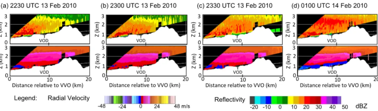
Doppler velocity (Fig. 3) in that region suggested a strong correlation be-100
tween the rapid cooling of the surface air and the change in the direction 101
of the valley flow. In particular, it showed a transition from up-valley flow 102
prior to the onset of the rapid decrease in surface air temperature and to 103
down-valley flow when the surface temperature reached 0◦C (Fig. 3). The 104
wind blows down valley flow the depth of the initial melting layer near the 105
surface approximately 150 min after the onset of precipitation. The radar 106
data used is discussed in (Joe et al., 2014). 107
2.2. Model setup 108
2.2.1. Model description 109
All of the simulations in this study were performed using the Weather 110
Research and Forecasting (WRF) model, version 3.3.1 (Skamarock et al., 111
2008). The set-up involves a semi-idealized two-dimensional configuration, 112
with modified orography corresponding to the Callaghan Valley area. The 113
initial conditions and inflow lateral boundary conditions were based on ob-114
servations of the case. The control run and the sensitivity tests with dif-115
ferent prescribed precipitation rates (described below) were done using a 116
two-moment bulk microphysics scheme as described in Milbrandt and Yau 117
(2005b) (hereafter referred to as MY2). Given the sensitivity to the param-118
eterization of snow shown in Milbrandt et al. (2014), it should be noted that 119
the original version of the scheme has been used in this study. 120
The two-dimensional transect of interest is a vertical cross section oriented 121
north-south passing through the radar location (VVO) and the Callaghan 122
Valley (VOD) (Fig. 1b). The orography around the VOD station was cen-123
tered in the domain; with 30 km of simplified orography, 60 km of flat ter-124
rain upwind (south of VOD), and 140 km downwind. The orography field is 125
smoothed six times with a 1-2-6-2-1 filter and then interpolated to a 250 m 126
grid spacing. The smoothing is necessary to remove numerical noise. For nu-127
merical stability at the time of model set-up, the elevation of the downwind 128
side of the mountain was fabricated to continue the mountain topography. 129
This prevents having an abrupt variation of the orography at the base of the 130
mountain. The result is a near-bell shaped mountain (Fig. 4a) similar to 131
that used in the default WRF idealized two-dimensional case. 132
The domain was chosen to be sufficiently large to minimize reflections 133
from the lateral boundaries. Hence, the domain was set to 200 km with 134
a 250 m grid spacing. The inflow and outflow boundaries were both set 135
to open. To have a maximum number of vertical levels within the melting 136
layer, 72 vertical grids have been used where the grid spacing varied from 137
20 m to 750 m for the z <9 km and 750 m for z >9 km. The top of the 138
atmosphere is at 22 km. To minimize reflections from the lateral boundary, 139
a 10 km damping layer was used at the top of the model to minimize the 140
reflection of gravity waves from the upper boundary (Klemp et al., 2008). 141
The simulation was integrated with time steps of 1 s for a total of 8 h. 142
The Coriolis force and surface fluxes have been neglected in the simulations. 143
All clouds and precipitation are represented by the microphysics scheme, 144
which varies according to the experiment. No subgrid-scale condensation or 145
convective schemes were used. 146
Note that the two-dimensional nature of our runs neglects the effects of 147
the valley geometry on the thermodynamic and dynamic evolution of the 148
valley atmosphere. For instance, in valleys with sloping side-walls a volume 149
effect occurs that causes the valley to cool more rapidly by melting than a 150
plain or a valley with vertical walls (e.g. Steinacker, 1983; Unterstrasser and 151
Z¨angl, 2006). Thus by neglecting three-dimensional valley geometry we are 152
likely underestimating the cooling rate of the valley air. 153
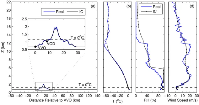
2.2.2. Initial conditions 154
The vertical temperature profile measured from VOC at 0000 UTC and 155
0600 UTC are shown in Fig. 5. At 0000 UTC, a shallow melting layer was 156
present near the surface and 6 h later, that melting was replaced by a near 157
0◦C-isothermal layer (Fig. 5b). Note that the wind direction also changed 158
with time and elevation. For example, the flow changed from southerly wind 159
to northerly wind between 0000 UTC 14 February 2010 and 0600 UTC 14 160
February 2010 at lower levels but stayed from the south at higher levels. 161
The meteorological fields were initialized using the Whistler (VOC) sound-162
ing at 0000 UTC 14 February 2010 (Fig. 4 b-d). We assumed that the 163
meteorological conditions were similar in the Callaghan Valley at the onset 164
of precipitation. Note that the Callaghan Valley is located south-west of the 165
Whistler sounding station (VOC) and that VOT observed the rapid cooling 166
of air temperature 2 h later than in Callaghan valley. The observed meteoro-167
logical fields were smoothed to prevent numerical instabilities. A comparison 168
of the real and smoothed temperature, relative humidity and horizontal wind 169
speed vertical fields are shown in Figs. 4b, c and d, respectively. To pre-170
vent snow sublimation aloft, the relative humidity has been increased to 95 171
% where the snow field is initialized (section 2.3). Finally, the north-south 172
component of the wind speed was used. 173
For the control run, the MY2, which predicts the mixing ratio and to-174
tal number concentration of 6 hydrometeor categories: clouds droplets, rain, 175
pristine ice crystals, snow, graupel and hail, was used. From the precipita-176
tion sensor located at VOT, the precipitation rate was around 3 mm h−1 but 177
the quantitative precipitation forecast (QPF) suggests that more precipita-178
tion occurred in the Callaghan Valley (VOD) (Th´eriault et al., 2012). We 179
based our assumptions on QPF because no precipitation sensor was installed 180
at VOD. Therefore, it was assumed that snow is falling continuously from 181
above the melting layer to yield a surface precipitation rate of approximately 182
5 mm h−1. The snow field was initialized with a mixing ratio, qs = 1.25 g
183
kg−1, and total number concentration, Ns = 9860 m−3, at the model level
184
corresponding to an elevation of 2.3 km, based on observed radar reflectiv-185
ity and temperature, assuming the relation between the snow intercept size 186
distribution parameter and temperature from Thompson et al. (2004) (see 187
Milbrandt et al. (2014) for details). 188
2.3. Sensitivity experiments 189
First, to show the impact of the temperature feedback from melting snow 190
on the direction of the valley flow field, the control run was run while neglect-191
ing the temperature tendency due to melting snow. This sensitivity experi-192
ment has been repeated with another microphysical scheme, the Thompson 193
et al. (2008) referred to as THOMP. Furthermore, we also repeated the con-194
trol simulation with a bin microphysics scheme (e.g. Geresdi, 1998; Geresdi 195
et al., 2014) referred as GERBIN. However the experiment neglecting the 196
temperature feedback from melting was not performed due to the complex-197
ity of the scheme. 198
Second, the initial precipitation rates were varied to determine the sen-199
sitivity on the time at which the flow reversal/stagnation is reached. In 200
weather forecasting in British Columbia, a rule of thumb is commonly used 201
(Trevor Smith, personal communication Environment Canada, 2010) that a 202
precipitation rate of 3 mm h−1 or more may lead to a valley flow reversal 203
in complex terrain. The investigation of the precipitation rate thresholds 204
associated with the change of direction of the valley flow is conducted for 205
many initial snow mixing ratio, qs = 2.5, 1.875, 1.25, 0.625, 0.3125 g kg−1,
206
corresponding approximately to resulting surface precipitation rates of 10, 207
7.5, 5, 2.5 and 1.25 mm h−1, respectively. The initial wind speed will also 208
affect the change in the direction of the valley flow field but only the initial 209
precipitation rate has been studied. For each initial snow mixing ratio (or 210
precipitation rate), the timing of the flow reversal at different stages was 211
investigated by comparing the location of the 0◦C-line on the mountainside 212
as well as the location associated with mixed precipitation types (50% snow 213
and 50% rain). 214
3. Impact of melting snow on the valley flow field 215
3.1. Control simulation 216
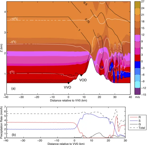
To ensure that the model reproduced acceptable atmospheric conditions 217
we have studied the weather conditions at 60 min. This time was chosen 218
because the 0◦C-isotherm is located approximately between VVO and VOD 219
(Fig. 6). The top panel shows the vertical cross-section of the wind, temper-220
ature, and snow fields and the bottom panel the surface precipitation rates 221
along the domain cross-section. First, the maximum simulated wind speed 222
is in excess of 20 m s−1 above the barrier between 2 and 4.5 km. At this 223
time, the wind at VVO remained in the up-valley direction but had started 224
weakening with respect to the initial conditions. Second, the 0◦-isotherm 225
reached the ground approximately 5 km north of VVO on the mountainside. 226
It has lowered by 400 m within 60 min in the simulations. Third, the snow 227
field is initiated upstream of the barrier at altitude between 2.3-6 km with a 228
mixing ratio value decreasing with height. The mixing ratio was chosen to 229
yield a precipitation rate of 5 mm h−1 on the upstream side of the mountain. 230
Snow is advected up to 50 km downstream of the barrier by the southerly 231
wind. Note that the rain and graupel fields aloft are not shown here because 232
a specific attention is paid to the main atmospheric and precipitation fields 233
occurring over the domain. 234
The surface precipitation rates along the cross-section show a mixture of 235
rain and snow on the upstream side of the barrier (Fig. 6b). The precipita-236
tion changed to mainly snow with some graupel 5 km north of VVO, which 237
corresponds to the location of where the 0 ◦C-isotherm reached the ground. 238
Note that some graupel are produced by accretion with cloud droplets that 239
formed due to ascending air along the mountainside. Graupel are also formed 240
downwind, which is possibly caused by the updraft associated with gravity 241
waves. 242
Now that we have an overall view of the weather conditions along the 243
domain, the remaining analysis will focus on the horizontal distance in the 244
vicinity of VVO and VOD (-10 km <y <15 km) and up to an altitude of 3 245
km above sea level. 246
3.2. Effects of melting on the valley flow field 247
To assess the impact of melting snow on the direction of the valley flow 248
field, the temperature tendency due to the melting of snow was disabled in 249
the microphysics scheme and the simulation was re-run and compared with 250
the control run. A similar experiment was also conducted with the control 251
setup but with the temperature tendency due to evaporation and sublimation 252
suppressed. First, the impact of the processes are minor and were only 253
present at the beginning (first 20 min) of the simulation until the atmosphere 254
conditions are saturated. This was excepted since the atmosphere was so near 255
to saturation with respect to liquid water. 256
The impact of the cooling associated with the melting of snow is clearly 257
shown in Fig. 7. This illustrates the horizontal wind speed at two times 258
of interest, which are 120 and 210 min, during the simulation. These times 259
correspond to when the valley flow begins to change direction and when the 260
down valley flow is distributed throughout the depth of the melting layer, 261
respectively. The results are similar to the radar radial velocity fields at 262
times corresponding to the onset of the change of the valley flow direction. 263
For example, precipitation started at approximately 2230 UTC 13 February 264
2010 and the flow began to change direction 60 min later. Therefore, it took 265
90 min for the flow to change direction and fill the initial depth of the melting 266
layer. The simulations suggest there is also 90 min time lapse between the 267
start of the reversal and the moment when the valley flow field has entirely 268
changed direction. This timing is comparable to the observed radar-inferred 269
winds. Figure 7c and d show simulation results obtained when the diabatic 270
cooling due to melting snow is turned off. The direction and strength of the 271
valley flow remains constant throughout the simulation time. These results 272
suggest that the temperature feedback associated with melting snow has an 273
impact on the valley flow direction or stagnation. 274
Melting also affects the small-scale structure of the valley airflow. As 275
melting begins, the associated cooling is not uniform with height. This lo-276
calized cooling destabilizes the atmospheric profile (Findeisen, 1940). As a 277
result, shallow convection temporarily occurs within and below the melting 278
layer in our simulation. These can be seen in Fig. 8, which is discussed in the 279
next section. Such melting-induced convection has been simulated previously 280
using more idealized settings (e.g. Szyrmer and Zawadzki, 1999; Unterstrasser 281
and Z¨angl, 2006). While this has a notable but temporary effect on the valley 282
flow structure, it appears that convective overturning has little overall effect 283
on the rate at which the valley cools. This is consistent with the fact that 284
the two-dimensional simulation results are similar, in terms of temperature 285
changes and precipitation phase transition, to the one-dimensional results of 286
Milbrandt et al. (2014), where convection is absent. 287
3.3. Mechanisms of the valley flow stagnation and reversal 288
The above analysis demonstrates the connection between melting and the 289
valley flow, but what are the dynamical mechanisms whereby melting causes 290
the flow to stagnate and reverse? In our simulations the effects of surface 291
friction and Coriolis have been neglected. Thus, in a Lagrangian framework, 292
horizontal pressure gradients are the only term capable of decelerating the 293
horizontal momentum of an air parcel (baring substantial internal dissipa-294
tion). 295
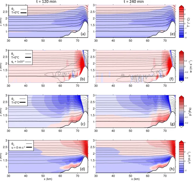
To analyze horizontal pressure gradients and their causes, Fig. 8 shows 296
perturbation fields from the control experiment at t =120 and 240 min. Tem-297
perature and horizontal velocity are plotted as anomalies with respect to the 298
initial profile. Pressure is plotted as an anomaly with respect to the p(z) 299
profile on the upwind boundary at the given time (to focus on instantaneous 300
horizontal pressure gradients). All panels also show contours of equivalent 301
potential temperature. These provide approximate streamlines where the 302
flow is reversible moist-adiabatic. The vertical gradient also provides an ap-303
proximate measure of the moist static stability. By t = 120 min, melting has 304
nearly cooled all the air at the base of the mountain to 0◦C, but at locations 305
further upwind there is still a substantial layer of above-freezing air with the 306
remnants of melting-induced convection. Within the melting-cooled air is 307
a zone of decelerated flow, centered at x = 60 km (Fig. 8a). A secondary 308
zone of deceleration is found further up the mountain slope. A high-pressure 309
anomaly of up to 0.5 Pa is found over the mountain slopes extending upwind 310
(Fig. 8c). As flow along streamlines crosses isobars, air parcels increase their 311
pressure and decelerate (Fig. 8d). Near z = 1 km streamlines rise over the 312
layer of cooled and decelerated air just upwind of the base of the mountain. 313
At t = 240 min the flow configuration is similar, except the low-level high 314
pressure anomaly and region of decelerated flow have expanded upwind past 315
x = 40 km (Fig. 8g-h). This is coincident with a deepening of the layer of 316
cooled air in the same region (Fig. 8e). Streamlines begin to rise far upwind 317
of the mountain to surmount this layer. 318
When the temperature effect of melting is suppressed in the simulations, 319
low-level cooling upwind is eliminated. A localized cool anomaly is still found 320
above the windward slope (Fig. 9). A high-pressure anomaly is still found 321
over the terrain, but it is confined to the upper portion of the windward 322
slope. Flow deceleration is found near 1.5 km but stagnation and reversal 323
do not occur. Near z = 1 km there is a localized acceleration of the flow 324
associated with the lifting of an upwind near surface jet of faster flow. 325
What is the source of the horizontal variations in the low-level pressure 326
anomaly that act to decelerate the flow and the differences between the sim-327
ulations? One plausible hypothesis is that horizontal variations in snowfall 328
rate above the melting layer lead to horizontal variations in melting-induced 329
cooling that produce (by hydrostatic balance) horizontal pressure variations. 330
Such horizontal variations in precipitation rate could be produced by oro-331
graphic enhancement. However, Fig. 6 shows that the total precipitation 332
rate is essentially uniform across the windward slope. Thus, while melting of 333
orographically enhanced snowfall may sometimes enhance flow deceleration, 334
such a mechanism does not explain the results of our experiment. 335
An alternative way to produce horizontal pressure gradients and decel-336
erate the flow is through the lifting of stratified air. In a stratified atmo-337
sphere, local lifting over the windward slope of a mountain produces cold-338
temperature and high-density anomalies. If the atmosphere is hydrostatically 339
balanced, these density anomalies directly result in high-pressure anomalies 340
beneath them that can cause the low-level flow to decelerate, stagnate, or 341
reverse (e.g. Smith, 1988, 1989). For uniform upwind conditions, simple ter-342
rain geometry, and in the absence of latent heating and Coriolis forcing the 343
occurrence of low-level flow stagnation is controlled by the horizontal aspect 344
ratio of the terrain and the non-dimensional mountain height: H = N h/U , 345
where N is the Brunt-Vaisalla frequency, U is the horizontal wind speed, and 346
h is the height of the terrain (e.g. Pierrehumbert and Wyman, 1985; Smith, 347
1989; Smolarkiewicz and Rotunno, 1990). This parameter measures the non-348
linearity of the flow and stagnation tends to occur above some threshold 349
value of H that depends on the terrain shape. In scenarios such as the one 350
we consider here, condensation of water vapor releases latent heat and mod-351
ifies the flow dynamics, reducing windward pressure perturbations and flow 352
deceleration. For flows of near-saturated air, the effects of condensation can 353
be roughly accounted for in the above theory by replacing H with a moist 354
non-dimensional mountain height Hm = Nmh/U (e.g. Jiang, 2003) where
355
Nm is a moist version of the Brunt-Vaisalla frequency (Durran and Klemp,
1982). 357
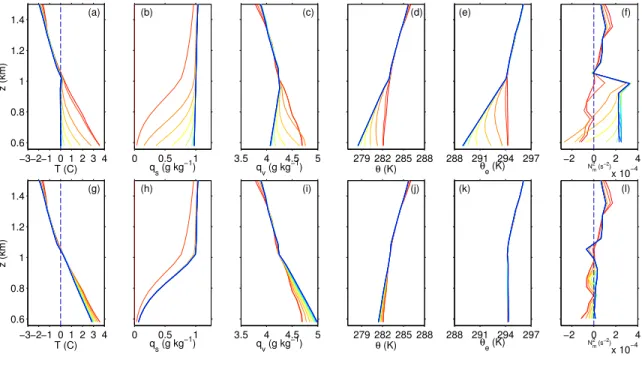
The interaction of the above mechanism with melting can be understood 358
by considering the evolution of the lowest 1 km of the atmospheric profile 359
upwind of the terrain (Fig. 10). Initially the low-level flow is unsaturated. 360
The profile is stable with respect to dry lifting, as evidenced by the profile 361
of θ (Fig. 10 d). Although Nm2 is initially slightly negative below z = 1 362
km (Fig. 10 f), since the flow is unsaturated, the profile is actually moist 363
stable, evidenced by the constant θe in the lowest 0.4 km. As the simulation
364
progresses, snow falls into the lowest layers and melts (Fig. 10 b). This 365
gradually cools the air below 1 km to 0◦C (Fig. 10 a). The cooling brings 366
this layer to saturation and excess water vapor is condensed out (Fig. 10 c). 367
This isothermal layer increases the dry stratification as represented by θ and 368
the moist stratification as represented by θe and Nm (Fig. 10 d-f). When the
369
temperature effect from melting is suppressed, only very modest amounts 370
of moistening and cooling occur in the lowest few hundred meters due to 371
sublimation (Fig. 10 g-i). These changes only cause slight modifications to 372
the upwind stratification (Fig. 10 j-l). 373
To explore changes in the dynamical regime associated with the observed 374
changes in the upwind profile, values of Hm are calculated before and after
375
melting. These are computed by averaging the horizontal winds and Nm of
376
the upwind profile from the surface to 2 km, and setting h=1.2 km. Before 377
melting Hm = 1.9. Although this is above the typical threshold of about
378
H=0.85 for flow stagnation for a two-dimensional ridge (e.g. Huppert and 379
Miles, 1969), our results are not directly comparable with previous studies 380
due to the non-uniform vertical profile. More importantly, the excess Nm
produced by melting increases Hmto 3.3, indicating that melting has changed
382
the upwind profile in such a way that flow stagnation is much more favored. 383
In the no-temperature effect from melting snow experiment sublimation Hm
384
only increases to 2.2, a much more modest change. 385
When the temperature effect of melting is suppressed, the lack of a sub-386
stantial pressure perturbation upwind of about x = 65 km is due to the 387
minimal lifting upwind of this region and lack of stratification below z = 1 388
km (Fig. 9 c and f). In this experiment the lifting-induced pressure anomaly 389
causes deceleration that is focused above 1.2 km (Fig. 9 g and h). When 390
melting is included the air below z =1 km becomes much more strongly 391
stratified (Fig. 8). Lifting of this melting-cooled air near the base of the 392
mountain produces a pressure perturbation, which produces much more sub-393
stantial flow deceleration (Fig. 8 c-d and g-h). As air upwind lifts over the 394
decelerated air, pressure anomalies are produced upwind of the foot of the 395
terrain (Fig. 8 c and g). As found in previous studies (e.g. Pierrehumbert 396
and Wyman, 1985) the region of decelerated flow propagates far upwind of 397
the mountain. In this and other two-dimensional simulations without Corio-398
lis forcing the upwind propagation continues indefinitely (Pierrehumbert and 399
Wyman, 1985). Eventually, the windward deceleration proceeds to the point 400
where the windward flow stagnates and reverses (Fig. 8 h). 401
In summary, melting modifies the windward flow dynamics primarily via 402
its effects on the upwind atmospheric profile. By stratifying the low-level 403
air, melting moves the flow into a dynamical regime with high Hm where
404
low-level pressure perturbations produced by lifting are able to decelerate 405
the flow to the point of stagnation and reversal. 406
4. Factors impacting the timing of the valley flow field 407
4.1. Cloud and precipitation microphysics parameterization approach 408
To examine the sensitivity to different parameterizations of snow, the 409
same experiments were run using two other microphysics schemes. They are 410
the THOMP bulk scheme, which has some notable differences in treatment 411
of snow compared to MY2, and the bin-resolving scheme (GERBIN). 412
Each microphysics scheme used in this study (MY2, THOMP and GERBIN) 413
is constructed differently but considers the same microphysical processes for 414
melting snow. These processes are (1) equilibrium between melting rate of 415
snow, condensational heating and diffusion of sensible heat by conduction; 416
(2) mass conversion from accretion and collection of cloud droplets and rain 417
drops in the melting layer. However, the behavior of each scheme in this 418
intercomparison is different because of specific basic assumptions such as ini-419
tial size distribution, number of moments predicted and characteristics of 420
categories. For example, the amount of mass converted into rain depends on 421
the atmospheric conditions (wet bulb temperature) but this equation is inte-422
grated over an analytic size distribution (for the bulk microphysics scheme). 423
Therefore, even if the atmospheric conditions are the same, the amount of 424
mass melted into rain depends on the parameters of the size distribution (N0
425
and λ) assumed. In the case of a bin microphysics scheme, the evolution of 426
the precipitation characteristics is highly detailed and considered to be more 427
realistic because there is discrete number of mass bins of snow. This allows 428
for a more accurate representation of the melting rate throughout the size 429
distribution of melting snow (Geresdi et al., 2014). Furthermore, the treat-430
ment of melted water is different between bulk and bin scheme approaches. 431
For instance, in the bin schemes no shedding occur as opposed to bulk scheme 432
where the melted water immediately sheds off the snowflakes. This difference 433
affects the number and the mean size of rain drops produced by the melting 434
process. 435
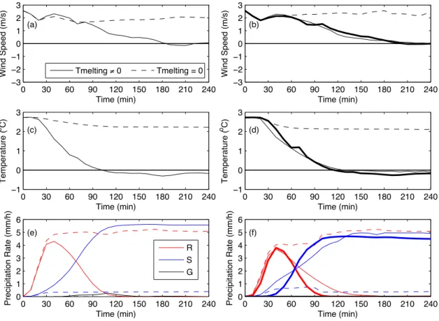
As shown in Figure 11, all microphysics schemes produced valley flow 436
stagnation in the control case. On the other hand, when the temperature 437
tendency from melting snow was shut off, none of the schemes produced a 438
change in the valley flow direction. We were able to disable the temperature 439
feedbacks from melting snow in the bulk scheme only due to the complexity 440
of the parameterization in a bin-resolving approach. Wind speed starts to de-441
crease 20 min after temperature starts to decrease, finally reaching 0 m s−1at 442
180 min, 210 min and 200 min for the MY2, THOMP and GERBIN, respec-443
tively. The wind speed and temperature remain nearly constant throughout 444
the time evolution when the cooling rate from melting snow is turned off 445
(MY2 and THOMP only). For a precipitation rate of 5 mm h−1, the wind 446
speed decreases to 0 m s−1 2.5 to 3 h after the surface temperature started 447
to decrease depending on the microphysics scheme used. 448
In terms of the surface temperature evolution, as expected, all micro-449
physics parameterizations show a cooling when the temperature feedback 450
from melting is considered. The temperature starts to decrease at the sur-451
face after 20 min in the simulation. This initial decrease in temperature 452
early in the simulations is likely due to evaporation and sublimation, as the 453
atmosphere is not yet saturated with respect to liquid water. The cooling is 454
mainly due to the temperature feedback from the melting of snow because it 455
eventually reaches a constant value of 0◦C at 100 min for the MY2 scheme 456
and 130 min for the THOMP and 110 for the GERBIN schemes. The timing 457
of the cooling rates is faster for the MY2 scheme because snow is assumed to 458
fall faster than in THOMP and GERBIN schemes. However, when snow falls 459
in the melting layer, its terminal velocity is doubled when falling at temper-460
ature above 0 ◦C in THOMP whereas it remains the same in MY2. In that 461
case, the residence time of snow in the melting layer is reduced which de-462
creases the melting rate and therefore the temperature feedback from melting 463
snow. Furthermore, the difference between the bin-resolving approach and 464
the bulk are the assumptions associated with the ice category transferred to 465
liquid water category. While the bulk schemes continuously produce water 466
drops by shedding snow and graupel, the bin approach forms water drops at 467
low concentration and of relatively larger size throughout the melting process 468
(Geresdi et al., 2014). In GERBIN the melted snowflakes are transferred to 469
the water drop category if the fraction of the melted water is larger than 0.85. 470
Note that when the temperature is near 0◦C even the smaller snowflakes do 471
not melt completely, which is not the case in the bulk approach. 472
This impact on the temperature evolution directly affects the types of 473
precipitation reaching the surface. As expected, when the temperature feed-474
back from the melting snow is neglected, the temperature and wind speed do 475
not vary significantly so a mixture of rain and snow is produced at VVO with 476
5 times more wet snow compared to rain. Only the MY2 scheme produced 477
graupel at the surface. This could be due to the decrease in the strength of 478
the vertical motion over the barrier, and in turn in the amount of available 479
cloud water to enable snow conversion to graupel. Also, the treatment of 480
snow conversion to graupel are different in THOMP and MY2 as MY2 tends 481
to generally produce more graupels than THOMP. For the case where full 482
microphysics is considered, a transition from rain to snow is produced at the 483
base of the mountain in addition to a trace of graupel between 60 to 150 min. 484
Note that the rate of transition from snow to rain is similar. For instance, 485
the time at which the precipitation type at the surface is half rain and snow 486
occurs between 68 and 80 min for all schemes. The differences are caused 487
by the different parameterization of snow and by the different treatment of 488
shedding in the three approaches tested. 489
4.2. Prescribed snow field aloft 490
The time evolution of the direction of the valley flow field and the timing 491
of the 0◦C line traveling along the mountainside have been studied by varying 492
the initial precipitation rate prescribed. This has been conducted only with 493
the MY2 microphysics scheme. These sensitivity experiments allow us to 494
address the following questions: (1) Is there a minimum precipitation rates 495
that would cause reversal or stagnation of the valley flow field? (2) What 496
is the relative timing of the 0◦C-line descending the mountainside and the 497
complete reversal of the valley flow? 498
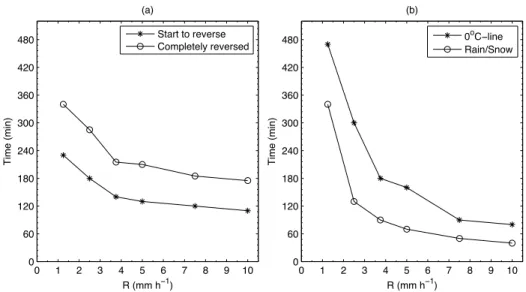
The change in the valley flow direction with full microphysics has been 499
studied for 6 prescribed precipitation rates. The times at which the valley 500
flow field starts to change direction and when the valley flow has completely 501
changed direction (<1 km ASL) have been calculated and are shown in Fig. 502
12a. The time at which the valley flow starts changing direction is defined by 503
the time at which the wind speed becomes negative below the 0◦C-isotherm 504
and between VVO and VOD. On the other hand, the timing associated with 505
completely reversed valley flow (<1 km ASL) was obtained based on the 506
maximum number of model grid points between VVO and VOD associated 507
with a negative wind speed. 508
First, the onset of the change in the wind direction occurs near the top 509
of the melting layer where cooling due to melting snow is present. As snow 510
continues to fall towards the surface, the change in the flow direction starts 511
to propagate downward. Second, all prescribed precipitation rates lead to a 512
change in the direction of the valley flow field but at different timings (Fig. 513
12a). Finally, the onset of direction change varies by 40 min from 1.25 mm 514
h−1 to 5 mm h−1 and this event occurs much faster for precipitation rates 515
>5 mm h−1. In particular, a precipitation of 10 mm h−1 has to be sustained 516
for nearly 2 h to start changing the direction of the valley wind whereas it 517
would take 4 h for a precipitation rate of 1.25 mm h−1. 518
Because of all the other processes influencing the temperature evolution 519
along the mountainside such as adiabatic cooling/warming, the complete 520
reversal of the flow occurred before the 0◦C-line reached the base of the 521
mountain. It takes nearly 360 min for the valley flow to completely change 522
direction at a precipitation rate of 1.25 mm h−1 and 180 min at 10 mm 523
h−1. Finally, the elapsed time between the onset of direction change and the 524
completion of the reversal increases with increasing precipitation rate. For 525
example, this time span is 65 min at 10 mm h−1 and 110 min at 1.25 mm 526
h−1. 527
Figure 12b plots the time when the 0◦C-line and the 50/50 rain/snow line 528
have, respectively, descended the mountainside under different precipitation 529
rates. As the precipitation rate increases, the time for the 0◦C-line to descend 530
the mountainside varied from 480 min for a 1.25 mm h−1 to 90 min for 10 531
mm h−1. The time for the 50/50 rain/snow line is shorter because that line is 532
located at lower elevation than the 0◦C-line. As expected, the time needed for 533
these lines to reach the base of the mountain is faster for higher precipitation 534
rate (10 mm h−1) than for lower ones (1.25 mm h−1). This is due to the fact 535
that low precipitation rate is associated with less mass melting into snow 536
and cooling off the top of the melting layer. Notice that the timing of change 537
in the flow direction and the timing of rain-snow boundary descending the 538
mountainside vary similarly. 539
The time associated with the change in the valley flow direction through-540
out the depth of the valley generally occurs after the 0◦C reached the base 541
of the mountain (Fig. 13). For example, the valley flow change direction 542
∼100 min after the 0◦C-line has reached the base of the mountain (VVO)
543
for a precipitation rate of 5 mm h−1. In this case, the onset of reversal and 544
the arrival of the 0 ◦C-line at the base of the mountain occur simultaneously. 545
On the other hand, the flow starts to reverse just when the 0◦C-line is still 546
going down the valley for a precipitation rate of 1.25 mm h−1. For the lowest 547
precipitation rate, the cooling rate is slower hence decreasing the lag time 548
between the cooling from melting snow and the change in the valley flow 549
direction. 550
5. Summary and conclusion 551
This study investigated the impact of the temperature feedback from 552
melting snow on the low-level flow field and precipitation phase transition 553
in complex terrain. In particular, experiments examining the temperature 554
feedbacks on the direction of the valley flow and the evolution of the rain-snow 555
line have been conducted. To address these issues, numerical simulations 556
using a semi-idealized setup have been used. The WRF model was initialized 557
with the vertical temperature, humidity and wind speed measured at VOC. 558
Snow was allowed to fall continuously from aloft at a constant rate on the 559
upstream side of the mountain, with no synoptic forcing. 560
A series of sensitivity experiments were conducted and the results showed 561
that the simulations with all of the microphysics schemes tested reproduced 562
a change in the valley flow field direction when the diabatic effect of melting 563
snow is considered. Although all schemes produced a slightly different timing. 564
Further sensitivity studies with different precipitation rates led to the 565
following conclusions: 566
• The timing of the flow reversal as well as the depth of the layer in 567
which it was produced was comparable to the radar data for the control 568
simulation. 569
• All precipitation rates tested produced a flow reversal/stagnation but 570
at different rates. However, the time to produce it is much longer for 571
lower precipitation rates. That means that calm synoptic conditions 572
need to be present of up to 8 h to observe a flow reversal produced by 573
a 1 mm h−1 snowfall rate. Since upwind evolution is key, adjusting 574
snow rate can only affect the timing of reversal, not its existence. Even 575
very light snowfall will eventually cool and stratify the air, leading to 576
reversal. However, in reality, only weak long lasting synoptic conditions 577
could lead to change in the flow direction in the valley. 578
• The speed of the rain-snow boundary traveling down the mountain 579
increases linearly with increasing the time for the valley flow to change 580
direction as the initial precipitation rate increases. It generally reaches 581
the base of the mountain before the flow reversal has completely fill up 582
the initial depth of the melting layer. 583
Further study should be conducted to verify the results with a full atmo-584
spheric model. It would be useful to study the impact of three-dimensional 585
valley geometry and the surrounding mountains on the timing of the flow 586
reversal. Also, an idealized study could be conducted to examine the rela-587
tive timing of large-scale warm air advection and cooling due to melting of 588
snow. For instance, given a synoptic forcing and a snowfall rate, one could 589
determine if the flow will reverse or not. 590
Overall, this study showed the importance that microphysical processes 591
can have on mesoscale flow and the conditions at the surface. This was 592
exemplified by the challenging prediction of local weather conditions during 593
the Vancouver 2010 Winter Olympics which was critical for safe and fair 594
competition. 595
Acknowledgments 596
We would like to thank the Natural Sciences and Engineering Research Coun-597
cil of Canada (NSERC) and the Fond Quebecois de la recherche sur la nature 598
et les technologies (FRQNT) for the financial support needed to accomplish 599
this work. The research made by N. Sarkadi and I. Geresdi was supported 600
by Hungarian Scientific Research Found (number: 109679). We would like to 601
acknowledge the contribution to constructive discussion with participants, in 602
particular Roy Rasmussen, at the 8th International Cloud Modeling Work-603
shop held in Warsaw, Poland in July 2012. The authors would like to ac-604
knowledge the SNOW-V10 principal and co-investigators for sharing the data 605
used in this study. 606
6. References 607
Barnett, T. P., Adam, J. C., Lettenmaier, D. P., 2005. Potential impacts of a 608
warming climate on water availability in snow-dominated regions. Nature 609
438, 303–309. 610
Durran, D. R., Klemp, J. B., 1982. On the effects of moisture on the brunt-v 611
aisa l a frequency. J. Atmos. Sci. 39 (10), 2152–2158. 612
Elsner, M., Cuo, L., Voisin, N., Deems, J., Hamlet, A., Vano, J., Mickel-613
son, K., Lee, S.-Y., Lettenmaier, D. P., 2010. Implications of 21st century 614
climate change for the hydrology of Washington State. Climatic Change 615
102 (1-2), 225–260. 616
Findeisen, C., 1940. The formation of the 0◦C isothermal layer and fractocu-617
mulus under nimbostratus. Meteorol. Z. 54, 49–54. 618
Geresdi, I., 1998. Idealized simulation of the colorado hail storm case: com-619
parison of bulk and detailed microphysics. Atmospheric Research 45, 237– 620
252. 621
Geresdi, I., Sarkadi, N., Thompson, G., 2014. Effect of the accretion by water 622
drops on the melting of snow flakes. Atmospheric Research, in press. 623
Henson, W., Stewart, R., Kochtubajda, B., Th´eriault, J., Sep. 2011. 624
The 1998 Ice Storm: Local flow fields and linkages to precipitation. 625
Atmospheric Research 101 (4), 852–862. 626
URL http://linkinghub.elsevier.com/retrieve/pii/S0169809511001645 627
Huppert, H., Miles, J., 1969. Lee waves in a stratified flow. Part 3: Semi-628
elliptical obstacle. Journal of Fluid Mechanics 35 (3), 481–496. 629
Isaac, G. A., Joe, P., Mailhot, J., Bailey, M., B´elair, S., Boudala, F., Brug-630
man, M., Campos, E., Carpenter, R., Crawford, R. W., Cober, S., Denis, 631
B., Doyle, C., Reeves, H., Gultepe, I., Haiden, T., Heckman, I., Huang, L., 632
Milbrandt, J., Mo, R., Rasmussen, R., Smith, T., Stewart, R. E., Wang, 633
D., 2014. Science of Nowcasting Olympic Weather for Vancouver 2010 634
(V10): A World Weather Research Programme project. SNOW-635
V10 Special Issue Pure and Appl. Geophys. 171, 1–24. 636
Jiang, Q., 2003. Moist dynamics and orographic precipitation. Tellus Series 637
A-dynamic Meteorology and Oceanography 55 (4), 301–316. 638
Joe, P., Scott, B., Doyle, C., Isaac, G. A., Cober, S., Mirecki, F., Gultepe, 639
I., Campos, E., Donaldson, N., Hudak, D., Stewart, R. E., 2014. The 640
monitoring network of the Vancouver 2010 Olympics. SNOW-V10 Special 641
Issue Pure and Appl. Geophys. 171, 25–58. 642
Klemp, J. B., Dudhia, J., Hassiotis, A. D., 2008. An upper gravity-wave 643
absorbing layer for nwp applications. Monthly Weather Review 136, 3987– 644
4004. 645
Lin, C. A., Stewart, R. E., 1986. Mesoscale circulations initiated by melting 646
snow. J. Geophys. Res. 91, 13299–13302. 647
Medina, S., Smull, B. F., R. A. Houze, M. S., 2005. Cross-barrier flow during 648
orographic precipitation events: Results from MAP and IMPROVE. J. 649
Atmos. Sci. 62. 650
Milbrandt, J., Th´eriault, J., Mo, R., 2014. Modeling the phase transition 651
associated with melting snow in a 1d kinematic framework: Sensitivity to 652
the microphysics. Pure and Applied Geophysics 171 (1-2), 303–322. 653
Milbrandt, J. A., Yau, M. K., 2005b. A multi-moment bulk microphysics 654
parameterization. Part II: A proposed three-moment closure and scheme 655
description. J. Atmos. Sci. 62, 3065–3081. 656
Minder, J. R., Durran, D. R., Roe, G. H., 2011. Mesoscale controls on the 657
mountainside snow line. J. Atmos. Sci. 68, 2107–2127. 658
Minder, J. R., Kingsmill, D. E., 2014/09/19 2013. Mesoscale variations of the 659
atmospheric snow line over the Northern Sierra Nevada: Multiyear statis-660
tics, case study, and mechanisms. Journal of the Atmospheric Sciences 661
70 (3), 916–938. 662
Pierrehumbert, R. T., Wyman, B., 1985. Upstream effects of mesoscale 663
mountains. J. Atmos. Sci. 42 (10), 977–1003. 664
Skamarock, W., Klemp, J., Dudhia, J., Gill, D., Barker, D., Duda, M., 665
Huang, X.-Y., Powers, J., 2008. A description of the advanced research 666
wrf version 3. Tech. rep., NCAR Techn. Note NCAR/TN-475+STR, 113 667
pp. 668
Smith, R., 1988. Linear theory of stratified flow past an isolated mountain 669
in isosteric coordinates. J. Atmos. Sci. 45, 3889–3896. 670
Smith, R., 1989. Mountain-induced stagnation points in hydrostatic flow. 671
Tellus 41a, 270–274. 672
Smolarkiewicz, P. K., Rotunno, R., 1990. Low froude-number flow past 3-673
dimensional obstacles .2. upwind flow reversal zone. J. Atmos. Sci. 47 (12), 674
1498–1511. 675
Steinacker, R., 1983. Diagnose und prognose der schneefallgrenze (diagnosing 676
and predicting the snowline). Wetter Leven 35, 81–90. 677
Steiner, M., O. Bousquet, R. A. H., Smull, B. F., Mancini, M., 2003. Air-678
flow within major alpine river valleys under heavy rainfall. Quart. J. Roy. 679
Meteor. Soc. 129, 411–431. 680
Szyrmer, W., Zawadzki, I., 1999. Modeling of the melting layer. Part I: dy-681
namics and microphysics. J. Atmos. Sci. 56, 3573–3592. 682
Th´eriault, J. M., Rasmussen, R., Smith, T., Mo, R., Milbrandt, J. A., Brug-683
man, M. M., Joe, P., Isaac, G. A., Mailhot, J., Denis, B., 2012. A case 684
study of processes impacting precipitation phase and intensity during the 685
vancouver 2010 winter olympics. Wea. Forecasting 27 (6), 1301–1325. 686
Thompson, G., Field, P. R., Rasmussen, R. M., Hall, W. D., 2008. Ex-687
plicit forecasts of winter precipitation using an improved bulk microphysics 688
scheme. Part II: Implementation of a new snow parameterization. Monthly 689
Weather Review 136 (12), 5095–5115. 690
Thompson, G., Rasmussen, R. M., Manning, K., 2004. Explicit forecasts of 691
winter precipitation using an improved bulk microphysics shceme. Part I: 692
Description and sensitivity analysis. Mon. Wea. Rev. 132, 519–542. 693
Unterstrasser, S., Z¨angl, G., 2006. Cooling by melting precipitation in alpine 694
valleys: An idealized numerical modelling study. Quarterly Journal of the 695
Royal Meteorological Society 132 (168), 1489–1508. 696
White, A. B., Gottas, D. J., Strem, E. T., Ralph, F. M., Neiman, P. J., 2002. 697
An automated brightband height detection algorithm for use with doppler 698
radar spectral moments. Journal of Atmospheric and Oceanic Technology 699
19, 687–697. 700
Z¨angl, G., 2007. Reversed flow in the south-alpine Toce valley during MAP-701
IOP 8: Further analysis of latent cooling effects. Q. J. R. Meteorol. Soc. 702
133, 1717–1729. 703
VOD
VOC
VVO
(a) (b)
VOT
Figure 1: (a) Western North America and (b) the Whistler area British Columbia. The Callaghan Valley is located at VOD, the radar was located at VVO and the soundings were launched from VOC. The precipitation rate shown in Fig. 2b was measured at VOT because no precipitation sensors were installed in the Callaghan Valley. Figure adapted from Th´eriault et al. (2012).
2100 UTC 13 Feb 0000 UTC 14 Feb 0300 UTC 14 Feb 0600 UTC 14 Feb ï5 ï2.5 0 2.5 5 Temperature ( o C)
(a) Temperature at VOD
2100 UTC 13 Feb0 0000 UTC 14 Feb 0300 UTC 14 Feb 0600 UTC 14 Feb
1 2 3 4 Precipitation Rate (mm h ï 1 ) Time (UTC)
(b) Precipitation rate at VOT
Figure 2: (a) The surface temperature evolution at VOD in the Callaghan Valley shows a rapid decrease in temperature. (b) The precipitation rate measured by FD12P at VOT, which is the base of Whistler Mountain. The onset of precipitation in the Whistler Area
!"# $"# %&'()*+,#-,.)/0,#(1#223#4567# "# "# !# $# 8#45 6 7# 23%# "# !# $# 9# 8#45 6 7# 23%# 9# !"# $"# %&'()*+,#-,.)/0,#(1#223#4567# "# "# !# $# 8#45 6 7# "# !# $# 9# 8#45 6 7# 23%# 9# 23%# !"# $"# %&'()*+,#-,.)/0,#(1#223#4567# "# "# !# $# 8#45 6 7# 23%# "# !# $# 9# 8#45 6 7# 23%# 9# !"# $"# %&'()*+,#-,.)/0,#(1#223#4567# "# "# !# $# 8#45 6 7# 23%# "# !# $# 9# 8#45 6 7# 23%# 9#
(a) 2230 UTC 13 Feb 2010 (b) 2300 UTC 13 Feb 2010 (c) 2330 UTC 13 Feb 2010 (d) 0100 UTC 14 Feb 2010
Legend: Radial Velocity
Reflectivity -20 -10 0 10 20 30 40 50 dBZ
Figure 3: The radar range-height indicator (RHI) of radar reflectivity (top panels) and radial doppler velocity (bottom panels). (a) is before precipitation started (b) is 30 min after the onset of precipitation (c) is when the valley flow starts to reverse and (d) is when the valley flow has completely change direction. This is a north-south cross-section looking northward from VVO into the Callaghan Valley.
ï60 ï40 ï200 0 20 40 60 80 100 120 140 2 4 6 8 10 12 14 16 18 20 22 T = 0oC (a)
Distance Relative to VVO (km)
Z (km) 0.5 0 10 20 30 1 1.5 2 2.5 VVO VOD T = 0oC Real IC ï60 ï40 ï20 0 (b) T (oC) 0 40 80 RH (%) (c) Real IC ï10 0 10 20 30 (d) Wind Speed (m/s)
Figure 4: An overview of the experimental design. (a) is the domain chosen and the real (blue) and smoother (black) topography. (b)-(d) are the observations measured by the sounding launched from VOC at 0000 UTC 14 February 2010 (fig 5a). (b) is the temperature, (c) is the relative humidity and (d) is the wind speed. The blue lines are the observed value and black are the WRF initial conditions.
−5 0 5 10 500 600 700 800 900 1000 Pressure hPa Temperature C (a) 0000 UTC 14 February 2010
−5 0 5 10 500 600 700 800 900 1000 Pressure hPa Temperature C (b) 0600 UTC 14 February 2010
Figure 5: The skew-T from Whistler area (VOC) at (a) 0000 UTC 14 February 2010 and at (b) 0600 14 February 2010.
Distance relative to VV0 (km) Z (km) 0oC −5oC −10oC 0.5 0.5 0.75 1 1 (a) VOD VVO −400 −30 −20 −10 0 10 20 30 40 1 2 3 4 m/s−15 −12 −9 −6 −3 0 3 6 9 12 15 18 21 24 27 −400 −30 −20 −10 0 10 20 30 1 2 3 4 5 6 7 Distance relative to VV0 (km) Precipitation Rate (mm/h) (b) R S G Total
Figure 6: Atmospheric conditions associated with the control run at 60 min. (a) The horizontal wind speed (filled contour), the temperature (white lines) and mass mixing
ratio of snow (g kg−1) (black lines) fields across the full horizontal domain but only up to
8 km above sea level. (b) The precipitation rate of snow, rain and graupel at the surface across the same domain.
Z (km) VOD (a) 0 5 10 15 20 0 1 2 3 m/s −15−12 −9 −6 −3 0 3 6 9 12 15 18 21 24 27 VOD (c) Distance relative to VV0 (km) Z (km) 0 5 10 15 20 0 1 2 3 VOD (b) Z (km) 0 5 10 15 20 0 1 2 3 VOD (d) Distance relative to VV0 (km) Z (km) 0 5 10 15 20 0 1 2 3 t =210 min t =120 min
Figure 7: The horizontal wind speed using the same color bar as the radar radial velocity to allow direct comparison. This is a sub-domain of Fig. 6 of comparable size to the radar image (Fig. 3) to facilitate the comparison of the fields. The top panels (a and b) are the control run, which includes all microphysical processes. The bottom panels (c and d) include the experiment suppressing the effect of cooling due to melting snow. The radar
is located at VVO at 0 km horizontal distance. The black line indicates the initial 0◦C
line. The left panels are the time associated with a change in the valley flow direction and the right panels are the time when the valley flow field has completely change direction.
t = 120 min t = 240 min −2 0 2 T′ (° C) 30 40 50 60 70 1 1.5 2 2.5 3 z (km) CTL56−1 zoom: 120 min −0.4 −0.2 0 0.2 w (m s − 1) 30 40 50 60 70 1 1.5 2 2.5 3 z (km) −0.2 −0.1 0 0.1 p (Pa) 30 40 50 60 70 1 1.5 2 2.5 3 z (km) −2 0 2 4 u (m s − 1) 30 40 50 60 70 1 1.5 2 2.5 3 x (km) z (km) −2 0 2 T′ (° C) 30 40 50 60 70 1 1.5 2 2.5 3 z (km) CTL56−1 zoom: 240 min −0.4 −0.2 0 0.2 w (m s − 1) 30 40 50 60 70 1 1.5 2 2.5 3 z (km) −0.2 −0.1 0 0.1 p (Pa) 30 40 50 60 70 1 1.5 2 2.5 3 z (km) −2 0 2 4 u (m s − 1) 30 40 50 60 70 1 1.5 2 2.5 3 x (km) z (km) θe T=0°C θe T=0°C qc = 1x10-‐6 θe T=0°C θe u = 0 m s-‐1 ‘ ‘ (a) (b) (c) (d) (e) (f) (g) (h)
Figure 8: Vertical sections showing perturbation fields from the control experiment. (a)-(d) show results at t = 120min. (e)-(h) show results at t=240min. (a) and (e) show
temperature perturbations with respect to the initial T (z, t0) profile. (b) and (f) show
vertical velocity. (c) and (g) show pressure perturbations with respect to the current
upwind profile p(z, t, xo). (d) and (h) show velocity perturbations with respect to the
initial u(z, t0) profile and a bold contour denotes regions of flow reversal. All panels
−2 −1 0 1 2 3 T′ (° C) 30 40 50 60 70 1 1.5 2 2.5 3 z (km) EXP56−2 zoom: 120 min −0.4 −0.2 0 0.2 w (m s − 1) 30 40 50 60 70 1 1.5 2 2.5 3 z (km) −0.2 −0.1 0 0.1 p (Pa) 30 40 50 60 70 1 1.5 2 2.5 3 z (km) −2 0 2 4 u (m s − 1) 30 40 50 60 70 1 1.5 2 2.5 3 x (km) z (km) −3 −2 −1 0 1 2 3 T′ (° C) 30 40 50 60 70 1 1.5 2 2.5 3 z (km) EXP56−2 zoom: 240 min −0.4 −0.2 0 0.2 w (m s − 1) 30 40 50 60 70 1 1.5 2 2.5 3 z (km) −0.2 −0.1 0 0.1 p (Pa) 30 40 50 60 70 1 1.5 2 2.5 3 z (km) −2 0 2 4 u (m s − 1) 30 40 50 60 70 1 1.5 2 2.5 3 x (km) z (km) t = 120 min t = 240 min θe T=0°C θe T=0°C qc = 1x10-‐6 θe T=0°C θe u = 0 m s-‐1 ‘ ‘ (a) (b) (c) (d) (e) (f) (g) (h)
Figure 9: As in Fig. 8, but showing perturbation fields from the no temperature feedbacks from melting snow simulation.
−3−2−1 0 1 2 3 4 0.6 0.8 1 1.2 1.4 (a) z (km) T (C) 0 0.5 1 (b) qs (g kg−1) 3.5 4 4.5 5 (c) qv (g kg−1) 279 282 285 288 (d) θ (K) 288 291 294 297 (e) θ e (K) −2 0 2 4 x 10⁻⁴ (f) Nm2 (s−2) −3−2−1 0 1 2 3 4 0.6 0.8 1 1.2 1.4 (g) z (km) T (C) 0 0.5 1 (h) qs (g kg−1) 3.5 4 4.5 5 (i) qv (g kg−1) 279 282 285 288 (j) θ (K) 288 291 294 297 (k) θ e (K) −2 0 2 4 x 10⁻⁴ (l) Nm2 (s−2)
Figure 10: Lower atmospheric profiles taken from upwind boundary. Profiles are plotted every 10 min from t = 0-240 min. Profiles from t=0 are red and successive profilers progress towards blue. (a)-(f) shows results from the control simulation. (g)-(l) show results from the no temperature feedbacks from melting snow simulation.
0 30 60 90 120 150 180 210 240 ï3 ï2 ï1 0 1 2 3 Time (min) Wind Speed (m/s) (a)
Tmelting & 0 Tmelting = 0
0 30 60 90 120 150 180 210 240 ï1 0 1 2 3 (c) Temperature ( o C) Time (min) 0 30 60 90 120 150 180 210 240 0 1 2 3 4 5 6 Time (min) Precipitation Rate (mm/h) (e) R S G 0 30 60 90 120 150 180 210 240 ï3 ï2 ï1 0 1 2 3 (b) Wind Speed (m/s) Time (min) 0 30 60 90 120 150 180 210 240 ï1 0 1 2 3 (d) Temperature ( o C) Time (min) 0 30 60 90 120 150 180 210 240 0 1 2 3 4 5 6 (f) Precipitation Rate (mm/h) Time (min)
Figure 11: The comparison of the surface (a) and (b) wind speed, (c) and (d) temperature as well as (e) and (f) precipitation rates of rain(R), snow (S) and graupel (G) at the base of the mountain (VVO). The results are obtained using the MY2 scheme (left column). The left columns are the results from the THOM microphysics scheme and the GERBIN micro-physics scheme (bold lines). The simulations with full microphysical processes (Tmelting 6= 0) and with suppressing the effect of cooling from melting snow (Tmelting = 0) are shown for MY and THOM but only the (Tmelting 6= 0) for the GERBIN.
0 1 2 3 4 5 6 7 8 9 10 0 60 120 180 240 300 360 420 480 R (mm hï1) Time (min) (a) Start to reverse Completely reversed 0 1 2 3 4 5 6 7 8 9 10 0 60 120 180 240 300 360 420 480 R (mm hï1) Time (min) (b) 0oCïline Rain/Snow
Figure 12: (a) The time needed for the valley flow field to start changing direction (Start to reverse) and to have changed direction throughout the depth of the melting layer at t = 0 (Completely Reversed) varying with the initial snow field aloft. (b) Time associated
0 60 120 180 240 300 360 420 480 0 60 120 180 240 300 360 420 480 Timing of 6 U (min)
Timing of rainïsnow boundary (min) Completely reversed Start to reverse
Figure 13: The relationship between the evolution of the valley flow field and the 0◦C
line reaching the base of the mountain. The dashed-line-circle is associated with the time needed for the valley flow field to start changing direction and the dashed-line-star is the time needed for the valley flow field to change direction throughout the depth of the melting layer at t = 0.