HAL Id: halshs-00667467
https://halshs.archives-ouvertes.fr/halshs-00667467
Preprint submitted on 7 Feb 2012
HAL is a multi-disciplinary open access archive for the deposit and dissemination of sci-entific research documents, whether they are pub-lished or not. The documents may come from teaching and research institutions in France or abroad, or from public or private research centers.
L’archive ouverte pluridisciplinaire HAL, est destinée au dépôt et à la diffusion de documents scientifiques de niveau recherche, publiés ou non, émanant des établissements d’enseignement et de recherche français ou étrangers, des laboratoires publics ou privés.
Real Exchange Rate and Economic Growth: Evidence
from Chinese Provincial Data (1992 - 2008)
Jinzhao Chen
To cite this version:
Jinzhao Chen. Real Exchange Rate and Economic Growth: Evidence from Chinese Provincial Data (1992 - 2008). 2012. �halshs-00667467�
WORKING PAPER N° 2012 – 05
Real Exchange Rate and Economic Growth: Evidence from Chinese
Provincial Data (1992 - 2008)
Jinzhao Chen
JEL Codes: O53, F31
Keywords: Real Exchange Rate, Economic Growth, China, Generalized method of moments
P
ARIS-
JOURDANS
CIENCESE
CONOMIQUES48, BD JOURDAN – E.N.S. – 75014 PARIS TÉL. : 33(0) 1 43 13 63 00 – FAX : 33 (0) 1 43 13 63 10
www.pse.ens.fr
Real exchange rate and economic growth: Evidence from
Chinese provincial data (1992–2008)
1Jinzhao CHEN*
*Paris School of Economics, France. E-mail: jichen@pse.ens.fr
Abstract
This paper studies the role of the real exchange rate in economic growth and in the convergence of growth rates among provinces in China. Using data from 28 Chinese provinces for the period 1992–2008 together with dynamic panel data estimation, I find conditional convergence among coastal provinces and also among inland provinces. The results reported here confirm the positive effect of real exchange rate appreciation on economic growth in the provinces.
JEL classifications: O53, F31
Keywords: Real exchange rate, economic growth, China, generalized method of
moments
1
This work was supported by Region Ile-de-France. I would especially like to thank Vincent Bignon for his help and suggestions during the time this paper was written. I am grateful also to Michel Aglietta, Philippe Jullian, and Wing Thye Woo for their valuable comments. I thank participants of the 2010 CES China Conference (Xiamen, June 2010), the Third Summer School on the Chinese Economy (Clermont-Ferrand, July 2010), the Lunch Seminar at the University of Paris West (Nanterre, January 2011), the DMM meeting (Montpellier, May 2011), the 16th World Congress of IEA (Beijing, June 2011), the 60th Congress of AFSE (Nanterre, September 2011), the 8th
International Conference on the Chinese Economy (Clermont-Ferrand, October 2011), and the 2012 ASSA Annual Meeting (Chicago, January 2012). I am deeply indebted to Joachim Jarreau, Iikka Korhonen, Romain Lafarguette, Barry Naughton, Xun Pomponio, and Thérèse Quang for discussions and suggestions that greatly improved the first version. For their constructive and valuable comments I gratefully acknowledge Mélika Ben Salem, Vincent Bouvatier, Matthieu Bussière, Eve Caroli, Marie-Françoise Calmette, Changsheng Chen, Cécile Couharde, Gilles Dufrénot, Ludovic Gauvin, Eric Girardin, Pierre-Cyrille Hautcoeur, Sylviane Guillaumont Jeanneney, Maria J. Herrerias, Jean Mercenier, Ronald I. McKinnon, Valérie Mignon, and Julie Subervie.
1 Introduction
Even though its breathtaking growth stalled in 2009, China has achieved a rapid recovery (recording a GDP growth rate of 8.7 percent) by its application of effective monetary and fiscal stimulus (ADB, 2010). However, spectacular and continual growth during the last three decades in China cannot hide the increasing disparity and inequality among the Chinese provinces (see Chen and Zheng, 2008; Heshmati, 2004; Xu and Zou, 2000).2 Wang and Hu (1999) even warned of possible severe consequences that could shake the political regime.
The increased spread in unconditional income distribution, as estimated by kernel density (see Jones, 1997; Quah, 1993; 1997) makes the point directly: there was a greater disparity in 2004 than in 1994 and 1984, when provincial disparity was already obvious (Figure 1a).3 Even after controlling for the effect of increasing average income (represented by rightward shifts of the distribution), the income distribution in logarithmic form (Figure 1b) reveals a similar pattern but with limited spreading; this implies a lower rate of increase in the proportional gap than in the absolute difference between rich and poor provinces.
[[INSERT Figure 1 about Here ]]
The regional disparity has long been a concern of policy makers and economists (Hu et al., 1995; NDRC, 2010). The country’s present economic development strategy generates considerable social tension because, over the past ten years, that strategy has proved largely incapable of reducing extreme poverty further or significantly improving the rural–urban and regional income imbalances (Woo, 2009). Furthermore, greater social and economic instability created by income disparities may obstruct the growth of China (Yang, 2002) and hence of other, low-income countries (Garroway et al., 2010)—given that, in the 21st century, China has contributed to global growth in general and to poor-country growth in particular. In this context, the issue at stake is whether or not managing the real exchange rate helps the Chinese government to rebalance economic growth and facilitate interprovincial convergence (whereby the poorest regions can benefit from development of the richest). In short: Does a lower real exchange rate spur provincial economic growth?
The real exchange rate (i.e., the relative price of tradable to nontradable goods) does not traditionally occupy a central role in growth regressions because it only recently entered theoretical models of economic growth.4 However, there has been a gradual recognition of the real exchange rate’s role in the growth process (see, e.g., Eichengreen, 2007; Rodrik, 2008). In fact, the disastrous effects of overvaluation on economic growth are widely documented in the
2
The geographical location and preferential policies of the Chinese government are identified as two main factors for the increase in this disparity (Démurger et al., 2002).
3
As a proxy for income, the real GDP per capita was calculated using the Chinese renminbi (RMB) at constant 2000 prices but adjusted to reflect purchasing power parity (PPP). The PPP for each
province is measured as the ratio of the provincial consumer price index (CPI) to the national one, which is taken as the benchmark (2000 is the base year). In contrast, Fleisher et al. (2010)
constructed the PPP in terms of a basket of goods in Beijing at constant 1990 prices.
4
The only exceptions are the works of Guillaumont Jeanneney and Hua (2001; 2008). However, their research mainly concerned the effect of the real exchange rate on urban–rural income inequalities, not on income itself or on economic growth.
empirical literature (Acemoglu et al., 2003; Benaroya and Janci, 1999; Cottani et al., 1990; Dollar, 1992; Gala, 2008; Ghura and Grennes, 1993; Loayza et al., 2004; Razin and Collins, 1997).5 There are fewer consensuses regarding the effects of undervaluation on growth. For Berg and Miao (2010), undervaluation—when viewed as a misalignment with long-run equilibrium levels—reduces growth. In contrast, Rodrik (2008) used an index of undervaluation that was adjusted for the Balassa–Samuelson effect and argued that undervaluation actually facilitates economic growth; however, this relationship holds only for developing countries. According to Rodrik, the growth-driven channel is the (usually dynamic) tradable sector, which contributes to innovations and productivity increases. For China, then, maintaining an undervalued currency could serve to subsidize its manufacturing industries, the driving force behind that country’s growth (Rodrik, 2010). Gala (2008) considered technological upgrading and capital accumulation as two main transmission channels. Overall, the real exchange rate can serve as a facilitating condition: it cannot by itself sustain economic growth, yet an appropriate exchange rate policy can make it easier for a country to capitalize on its growth opportunities (Eichengreen, 2007). Eichengreen also claimed that keeping the real exchange rate at competitive levels and avoiding excessive volatility are both important for growth.6
Despite a growing number of studies examining the link between the real exchange rate and economic growth across countries (for a comprehensive literature review, see Eichengreen, 2007), none considers the impact of real exchange rate of the RMB on economic growth in China at the provincial level. This paper attempts to fill that gap in the empirical growth literature by focusing on the rate’s impact on provincial economic growth and on the conditional convergence of growth rates among the provinces.
To investigate the impact of the real exchange rate level on provincial growth, I apply the growth regression of Barro (1991) to a panel data set of 28 Chinese provinces. The real exchange rate (RER) is often defined as the relative price of tradable to nontradable goods (or inversely)—as in the standard, two-sector framework of a small open economy in which each sector produces a different type of goods. The RER so defined, and used here, is also known as the ‘internal’ real exchange rate (Salter, 1959); an increase corresponds to a depreciation of the real exchange rate. Using dynamic panel estimations (with fixed effects model and the generalized method of moments estimation for system of equations, known as system-GMM estimation), I find a conditional convergence among the coastal provinces and among inland provinces for the period 1992–2008 but no convergence between these two groups of provinces. The results also show that an appreciation of the real exchange rate boosts provincial economic growth, which is not the same effect found by Rodrik (2008). The positive effect reported here could result from the redistribution of resources between sectors, the wealth effect stemming
5
For example, Ghura and Grennes (1993) showed a negative correlation between currency misalignments (overvaluation) and 33 sub-Saharan African countries’ economic performances. Goldfajn and Valdes (1996) argued that most balance-of-payments crises are related to overvalued currencies.
6
However, the evidence for a link between the exchange rate volatility (or variability) and economic growth is less definitive (Aghion et al., 2009; Ghura and Grennes, 1993). In addition, other narratives focus on the nexus between the exchange rate regime and growth; Levy-Yeyati and Sturzenegger (2003) found that less flexible exchange rate regimes are associated with slower growth in developing countries but that the choice of a particular exchange rate regime has no statistically significant effect on growth in industrial countries.
from enhancement of agricultural and service sectors, and/or the rising real wages and productivity of workers.
The paper is organized as follows: in section two, I present the empirical methodology and the specification of the informal growth regression; section three describes the variables chosen as determinants of China’s provincial economic growth and the new data to which the model is to be applied; I present in section four the results of regressions using different estimators and, before concluding, discuss in section five the transmission mechanism through which the role of the real exchange rate in growth takes effect.
2 Empirical methodology
The unconditional income distributions plotted in Figure 1 provide no evidence of economic convergence among the Chinese provinces. However, for a study of convergence it is more informative to examine the conditional distribution of per capita income. If the income gap became narrower over time between provinces sharing similar characteristics, then this would constitute conditional convergence; hence the provinces would converge to their respective steady states.
Despite a large body of literature seeking to explain China’s miraculous growth (e.g., Herrerias and Orts, 2011; Woo, 1999), the empirical findings have yielded no consensus on provincial growth convergence.7 Empirical research on China’s economic growth include a few studies that use the cross-country approach (with panel and/or cross-sectional data; see Ding and Knight, 2009; Li et al., 1998; Rodrik, 2008). There is a larger body of empirical studies that focus on the evidence of interprovince growth in China. Two main empirical approaches are in common use.8 The first amounts to variants of the neoclassical growth model, often the augmented Solow model pioneered by Mankiw et al. (1992).9 The second widely used approach incorporates informal growth regressions (Barro, 1991; Barro and Sala-i-Martin, 2004); with this approach, which is followed here, various economic theories of growth as used as a guide to choosing the right-hand-side (RHS) variables in the growth regression.
2.1 Informal growth regression
In this paper I follow the informal growth regression approach and implement the traditional linear informal growth regression analysis.10 The growth regression is written as
, , 1 ; ,
i t i t i t t i i t
y y X f f
(1)
for i = 1, …, N and t = 2, …, T. Here Δyi,t is the log difference in real per capita GDP over a
five-year period, yi,t−1 is the logarithm of real per capita GDP at the beginning of each period (a
proxy for initial income), X is a vector containing the explanatory variables measured either
7
See Maasoumi and Wang (2008) for a recent measure of convergence in China and a comprehensive literature review.
8
Another empirical approach is the growth accounting method; see Zheng et al. (2009) for an application to potential output in China.
9
See Chen and Fleisher (1996). Li et al. (1998) utilized both cross-sectional and panel data on the provinces of China.
10
Béreau et al. (2009) used the panel smooth transition regression (PSTR) model introduced by Gonzalez et al. (2005) to explore the nonlinear relationship between currency misalignment and economic growth for an extensive panel that included both industrialized and emerging economies.
during that period (period average) or at the beginning of it (period initial value), fi denotes
unobserved province-specific factors reflecting differences in the initial level of technical efficiency, and ft is a time-specific effect that captures the productivity changes common to all
provinces (see Cottani et al., 1990; Ding and Knight, 2009; Ghura and Grennes, 1993). Equation (1) can be rewritten as
, ( 1) , 1 ; ,
i t i t i t t i i t
y y X f f (2) for i = 1, …, N and t = 2, …, T, which is a dynamic panel data specification with a lagged dependent variable on the RHS.
The correlation between the lagged dependent variable and the time-invariant, country-specific effects renders the ordinary least-squares (OLS) estimator of equation (2) biased and inconsistent. Even with a fixed-effects estimator, the coefficient for initial income is likely to be seriously biased downward in a small sample with limited time span (Nickell, 1981). I therefore follow the recommendation of Bond et al. (2001) and use instead a system-GMM estimator, one with demonstrated superior performance on finite samples, developed by Arellano and Bover (1995) and Blundell and Bond (1998). This estimator uses moment conditions for a system, including both the first-differenced and the original equation in levels: lagged levels of the RHS variables are used as instruments in the first-differenced equations, and lagged first-differences are used as instruments in the original equation. Including the equation in levels in the system yields efficiency improvements as well as a significant reduction in the large bias suffered by the first-differenced GMM estimator (which results because the lagged levels of variables are only weak instruments for subsequent first differences).11 Moreover, Bond et al. claimed that the potential for obtaining consistent parameter estimates—even in the presence of measurement error and endogenous RHS variables—is a considerable strength of the GMM approach to empirical growth research.
3 Variables and data
In this section, I discuss the variables entering into the regression just described; I also present the data set and explain how the proxies for those variables are constructed.
3.1 Variables
The dependent variable is the growth rate of real income, as represented by the annual growth rate of the real GDP per capita for each Chinese province. With regard to the chosen explanatory variables for economic growth, a broad range of factors are taken into account. Given the relatively small number of observations (N = 28 and T = 4 when a sample averaged over five years is used) and in order to guarantee enough degrees of freedom for the estimation, only a few proximate determinants were chosen.12 These explanatory variables of economic growth rate are widely identified in the literature of economic growth.
First, the conditional convergence hypothesis argues that, ceteris paribus, countries with lower per capita GDP grow more rapidly owing to higher marginal returns on capital stock.
11
The downside is the need to add more instruments to the estimation.
12
Even some potentially explanatory variables of growth are not included in the regression. Note that panel data methods can control for omitted variables.
Hence I included the initial level of real per capita GDP to control for such conditional convergence (Barro and Sala-i-Martin, 2004).
Second, the X vector includes the ratio of investment to GDP (based on the neoclassical model of Solow, 1956) and also the population’s natural growth rate. Growth is expected to be positively associated with investment and capital accumulation but negatively associated with population growth.13
Third, it is widely hypothesized that human capital has a positive effect on economic growth (see Lucas, 1988). Chen and Fleisher (1996), Fleisher and Chen (1997), and Démurger et al. (2002) provide evidence that education at the secondary or collegiate level helps account for observed differences in Chinese provincial growth rates. However, there is no agreement on the indicators for measuring such capital. Early proxies for human capital consisted of measuring the rate of gross secondary school enrollment (see Barro, 1991; Bond et al., 2001; Caselli et al., 1996; Mankiw et al., 1992). Alternatively, Ding and Knight (2009) relied on the ‘average level of human capital’ data provided by Barro and Lee (2001) to calculate the average years of schooling in the population (above age 15) as a direct measure of the stock of human capital. That approach might be preferable because school enrollment rates may conflate human capital stock and accumulation effects and because such rates are often a poor proxy for either factor (Gemmell, 1996; Temple, 1999).14 So in addition to using the gross secondary enrollment rate, I follow Fleisher et al. (2010) and calculate the fraction of those in the total population who have at least a senior high school education as another proxy for the stock of human capital.15
A major force pushing the economy toward marketization has been the introduction of foreign ownership through foreign direct investment (FDI) (Fleisher et al., 2010). Through its potential to bring in new production and managerial technologies, FDI has facilitated the transformation of China’s state-owned and collective sectors (Liu, 2008). I incorporate this variable to help explain regional economic disparities.
Furthermore, a policy variable—trade openness—is also included.16 This variable is viewed as having a positive role on economic growth and poverty reduction not only in neoclassical trade models (via comparative advantage) but also in the endogenous growth literature (via diffusion of technology or economies of scale). However, a large number of studies have yielded different empirical findings and various explanations (see Dufrénot et al., 2010).
13
This variable is different from the one in Solow’s growth model, where the population growth was measured by the rate of growth of the working-age population (and taken exogenously), emphasizing the supply of labor. In this paper, population growth is taken to be endogenous—as in endogenous growth theory, where population growth is negatively associated with growth in human capital and hence with economic growth (Bond et al., 2001). The fertility rate is often used as an alternative measure of population growth (Barro, 1991).
14
Ding and Knight (2009) also adopted the estimates of Yao (2006), who treated each year’s school graduates as an addition to the human capital stock.
15
Here, the senior high school includes the special technical secondary school (Zhong zhuan in Chinese) but not the skill school (Ji Xiao). The numbers of people with at least some college education and with at least some senior high school education are estimated based on the respective annual flows of enrollments in college and senior high school; these numbers are anchored to periodic population census data and annual population change survey data. The census data (1982, 1990, and 2000) and the annual population change survey data (1993, 1996, 1999, 2002, and 2003) provide the proportions of people sorted by their educational levels.
16
One could also introduce other variables (e.g., inflation) that reflect macroeconomic stabilization policies and institutions.
It could be argued that the regional divergence (or disparity) in incomes noted in previous studies may be due largely to geographic (or location) factors (Chen and Fleisher, 1996; Démurger et al., 2002). Furthermore, the differences in preferential open-door policies at the provincial level might also lead to growth disparity. These two factors may combine to yield a direct effect on the openness of trade as well as an indirect effect on other sources of growth (e.g., technological progress) via attracting foreign investment. By giving each province a weight that reflects the type of economic zone that it hosts, Démurger et al. constructed an annual index of the level of open-door preferential policies; that index ranges from 0 to 3 for each province during the period 1978–1998, where 3 corresponds to the highest level of central government’s policy preference. In addition to these indexes, a simple period average for each province is reported (see Table 4 of their paper).17 Pedroni and Yao (2006) divided these provincial average indexes (which range from 0.33 to 2.86) into three roughly equal quantiles: low, medium, and high (see Table A2 in the Data Appendix). In the regressions reported here, I include the variable of policy preference level in the categorical form of Pedroni and Yao.18
I introduce the variable of interest—the real exchange rate of Chinese provinces—in order to investigate the impact of rate changes on China’s economic growth. Measuring the real exchange rate is not straightforward, and the difficulties are both conceptual and empirical. The many and varied definitions of the real exchange rate, which are drawn from different analytical frameworks and suitable for use in different circumstances, have long complicated the analysis of real exchange rate issues (Montiel and Hinkle, 1999).19 I adhere to the standard framework and directly measure an internal real exchange rate for each of the 28 Chinese provinces. This rate is defined as the relative price of tradable to nontradable goods, expressed in logarithmic form: ln RERln(PT/PNT).20
3.2 Data
The empirical literature on growth in developing countries is rife with inaccurate data and measurement error. Sometimes, data falsification results from political influence.21 Since there is no alternative data set to the official series for China (see Naughton, 2007, p. 141), researchers
17
Various types of economic zones reveal that the provinces benefited disproportionately from this open-door policy, which consisted of attracting FDI and promoting foreign trade in targeted economic zones. A weight of 3 was assigned to the Special Economic Zone (SEZ) and Shanghai Pudong New Area; a weight of 2 was assigned to the Economic and Technological Development Zone (ETDZ) and Border Economic Cooperation Zone (BECZ); and a weight of 1 was assigned to the Coastal Open City (COC), Coastal Open Economic Zone (COEZ), Open Coastal Belt, major city on Yangtze (MC), bonded area (BA), and capital city of inland province or autonomous region (CC). A weight of 0 was assigned to each province without an open zone.
18
See also Maasoumi and Wang (2008), who included the policy preference level in this form.
19
Montiel and Hinkle (1999) remark that the empirical measurement of RER in most developing countries involves many practical problems that are seldom encountered in the case of industrial countries.
20
One could instead take the real effective exchange rate (a.k.a. the ‘external’ real exchange rate) as a proxy for the real exchange rate, as in Guillaumont Jeanneney and Hua (2008).
21
For influential work on the reliability of China’s GDP statistics, see (among others) Maddison (1998), Rawski (2001), and Holz (2006).
have no choice but to use official Chinese data while making, perhaps, some corrections and adjustments.
The empirical analysis in this paper is based on a data set compiled from several sources: the China Compendium of Statistics 1949–2008 (CCS), published in 2010; the China Statistical Abstract 2010 (CSA); various issues of the China Statistical Yearbook (CSY) and the China Population Statistical Yearbook (CPSY); and the China Population and Employment Statistics Yearbook 2009 (CPESY). An important feature of this study is my use of relatively recent official data to construct a new series of real GDP per capita, for each province, that takes into account the second national economic census of 2008. Hence the GDP series employed here are assumed to be better (i.e., less biased) than those used in previous studies.22
The annual sample includes 28 provinces for the period 1992–2008.23 For the panel data study, I obtained a data set for each province that was averaged over a nonoverlapping five-year interval to mitigate the influence of temporary factors associated with business cycles.24
The dependent variables are the five-year average growth rates g of real GDP per capita; the annual rates are plotted in Figure 2.25 These growth rates are deflated (by provincial CPI) and calculated in terms of constant 2000 RMB. The proxies for the explanatory variables entered into the regression are as follows. The logarithm of real GDP per capita at the beginning of the five-year period (ly_1) as the proxy for the initial level of income; the share of the gross capital formation in GDP (invest2gdp1) and the share of the fixed capital formation in GDP (invest2gdp2) as proxies for investment share; the ratio of gross secondary school enrollment to total population (school1) and the share of those who have at least some senior high school education (school2) as proxies for human capital; the population’s natural growth rate (popgr) as the proxy for population growth; the share of FDI in GDP (fdi2gdp) and in gross capital formation (fdi2invest) as proxies for FDI share; and the ratio of total international trade, both export and import, to GDP (trade2gdp) as the proxy for trade openness.
[[INSERT Figure 2 about Here ]]
22
The current-price GDP series for 2005–2008 that are published in 2010 CSA have been revised to reflect the second economic census; the series published in CSY report preliminary figures only (which are nevertheless used in some studies).
23
From the administrative standpoint, mainland China consists of 31 provinces, minority autonomous regions, and municipalities. Because Chongqing became a municipal city in 1997, we combined Chongqing with Sichuan for the period 1997–2006 to preserve consistency with earlier observations (cf. Ding and Knight, 2008). Hainan and Tibet are excluded because so few data are available for their PPI indices.
24
This is a commonly adopted practice in the empirical growth literature; see Islam (1995), Bond et al. (2001), Bussière and Fratzscher (2008), and Ding and Knight (2008; 2009). The limited span of the series explains my choice of five-year intervals (1992–1996, 1997–2001, 2002–2006), although the fourth period (2007–2008) allows only for two-year averages. See Hao (2006) for a study in which period-averaged data is based on a three-year interval. One should bear in mind that it is an open question whether using five- or ten-year averages for avoiding business cycle effects or annual data is better. Further investigation is needed on the extent to which averages taken over short time spans reduce such effects (cf. Temple, 1999).
25
The growth rate for Sichuan includes an outlier that is due mainly to the difficulty of calculating a reliable year-end population for this region in 1997, when Chongqing became a municipal city.
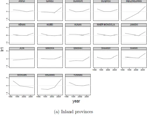
For the location variable, I use a simple indicator set equal to 1 for coastal provinces and to 0 otherwise (Ding and Knight, 2008).26 For the level of policy preference, I create two dummy variables (policy_dum2 and policy_dum3) based on the categorical variable (policy_var) reported in Pedroni and Yao (2006) and introduce them into the GMM estimation. Finally, I add trade openness—defined as the ratio of total international exports and imports to GDP (trade2gdp)—as well as the real exchange rate, which is measured not only by the logarithm of the relative price of tradable to nontradable goods (lr1, see Figure 3) but also by the logarithm of the inverse of the price of nontradable goods (lr2).27 The prices of tradable goods (PT) and
nontradable goods (PNT) are represented, respectively, by the producer price index28 and the
consumer price index.29
[[INSERT Figure 3 about Here ]]
All the variables are plotted in Figure 4, and their definitions and sources are summarized in Table A1.
[[INSERT Figure 4 about Here ]]
4 Results
The Im–Pesaran–Shin panel unit root test (Im et al., 2003) is applied to check the stationarity of the annual series of each variable from 1992 to 2008 (see Table 1).30 Except for the growth rate, FDI share, and RER, the null hypothesis of nonstationarity cannot be rejected.
Table 1. Im–Pesaran–Shin panel unit root test
Variable t-bar statistics p-value Observations
g −2.402 0.000 420
g (no Sichuan) −2.356 0.000 405
ly_1 −2.231 0.367 420
ly_1 (no Sichuan) −2.213 0.408 405
invest2gdp1 −2.079 0.705 420 invest2gdp2 −2.447 0.057 420 popgr −2.190 0.458 420 school1 −1.878 0.954 420 school2 −2.338 0.183 420 open −1.831 0.975 420 fdi2gdp −3.704 0.000 420 fdi2invest −3.385 0.000 420 lr1 −2.713 0.001 420 lr2 −2.541 0.017 420
Notes: All variables are demeaned. For g, only the constant is included; for other
variables, both the trend and the constant are included. The test is augmented by one lag.
26
For a more precise classification of Chinese provinces’ locations, see Démurger et al. (2002). 27
If one assumes that the prices of tradable goods are the same for all provinces. 28
In China, the PPI is referred to as the Producer Price Index for Manufactured Goods.
29
Edwards (1990) and Devereux and Connolly (1996) used the CPI as a proxy for the price of nontraded goods.
30
4.1 Estimations with fixed-effects model
Because some variables are nonstationary, I implement panel estimations on the data set at five-year intervals rather than performing pooled OLS estimation. The results for the baseline model—which includes initial income, the investment ratio, the population’s natural growth rate, and the rate of secondary school enrollment—are reported in Table 2. Based on the Hausman specification test (Hausman, 1978), I choose the fixed-effects model and then estimate equation (1) on three samples (all provinces, the inland ones, and the coastal ones) using two proxies for the ratio of investment and two for human capital. Except for the variable of human capital (see the coefficients for school1), every explanatory variable of economic growth is correctly signed; however, the significance levels are not always sufficient to validate the assumptions. Among these regressions,31 the significance of the initial income per capita (ly_1) indicates that there is conditional convergence for the coastal provinces and the whole sample but not for the group of inland provinces. However, the ratio of investment to GDP (invest2gdp1 and invest2gdp2) and the population’s natural growth rate (popgr) are significant for the whole sample and for the inland provinces, too. As for human capital, only the proportion of those with at least a senior high school education (school2) is significant—and only for the inland provinces.
[[INSERT Table 2 about Here ]]
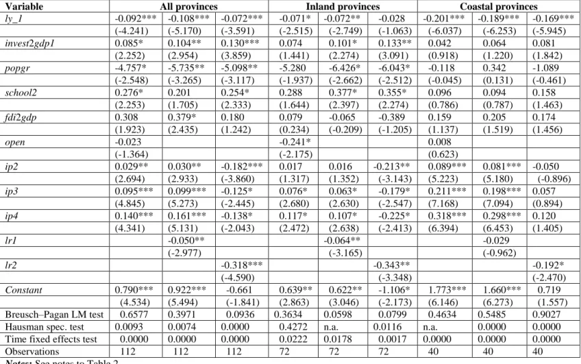
Next I incorporate the explanatory variables (e.g., FDI, trade openness, RER) into the growth regression; the results are reported in Table 3. There are two main differences relative to the baseline model reported in Table 2. First, the results indicate a conditional convergence for all three samples. Second, the effect of human capital on growth is significant for the sample as a whole and also for the inland provinces. In other words, it is not human capital that drives the economic growth of the most dynamic coastal provinces. This finding may be explained by drawbacks of using within estimator under conditions of endogenous explanatory variables and possible measurement error. The latter condition is more prevalent in developing countries, such as China. Similar negative and/or nonsignificant coefficients for human capital are also reported by Romer (1989) and by Levine and Renelt (1992).
[[INSERT Table 3 about Here ]]
Neither foreign direct investment nor trade openness is significantly associated with the disparity in economic growth among Chinese provinces. As for the trade openness, one possible explanation for its relative nonsignificance is the heterogeneity of the variable’s parameters—that is, the dependence of the trade–growth relation on where a province lies in the distribution of per capita growth.32 Finally, the real exchange rate is negatively associated with economic growth; this impact is significant in nearly all the regressions. In other words: when the real exchange rate appreciates (i.e., when the tradable/nontradable price ratio decreases), the economy grows more quickly.
31
For each sample, three regressions are run using alternative proxies for the investment ratio and for human capital.
32
To be precise, openness has a greater impact on growth among low-growth than among high-growth provinces (Dufrénot et al., 2010).
4.2 Regressions with system-GMM estimator
Given the drawbacks of fixed-effects estimators aforementioned in section 2.1, the literature on economic growth has seen the wide application and continued development of GMM estimation. Here I implement the one-step system-GMM estimator via the ‘xtabond2’ module of Stata 10 (Roodman, 2003).33 The p-values of Hansen tests indicate the overall validity of the instruments used in all models presented in Table 4. The Arellano–Bond AR (2) test confirms that the differenced error term is not second-order serially correlated. (By construction, the differenced error term is probably first-order serially correlated; this is suggested by the p-values of the Arellano–Bond AR(1) test.)
[[INSERT Table 4 about Here ]]
Table 4 presents the results of this dynamic panel specification. Model 0 is the baseline model estimated via the system-GMM estimator. Model 1 (resp., 1a and 1b) adds the real exchange rate (resp., lr1 and lr2). Model 2 (resp., 2a and 2b) is the same as Model 0 but adds dummy variables for location and policy preference level (resp., loca_dum, and policy_dum2 and policy_dum3). Model 3 (resp., Model 4) includes the real exchange rate lr1 (resp., lr2) and the location dummy in addition to the control variables of Model 0; similarly, Models 5 and 6 add the real exchange rate and the policy preference level variable.
Three points are worth noting. First, the fundamental determinants of growth—such as investment rate (invest2gdp1) and human capital (school1)—are significant in most of these dynamic models: the former in all models and the latter in several. The location dummy and one of the dummies for policy preference level (policy_dum3) are also significant, which indicates that differences in location and in policy preference level (between the provinces receiving highest policy preference and the ones receiving lowest preference) have significant effects on growth. So other factors being equal, a coastal province will have a higher growth rate than an inland province and obtaining a greater preference from central government for opening SEZs will have a significant and positive effect on growth.
Second, introducing the location dummy and the policy preference level dummies reveals the existence of conditional convergence—among coastal provinces on the one hand and among inland provinces on the other hand; however, there is no convergence between these two groups of provinces.34 This confirms previous findings that geographical location and the Chinese central government’s preferential policies for locating SEZs both figure largely in the increasing disparity (Démurger et al., 2002).
Third, the real exchange rate is significant in several models when proxied by lr1 (but not by lr2). Thus, I focus on the relative price of tradable to nontradable goods that is proved be a better proxy of China’s real exchange rate.35 The coefficient for this variable is negative, which implies that an appreciation in the real exchange rate (that is the increase of the relative price of
33
In finite samples, asymptotic standard errors associated with the two-step GMM estimators may be strongly biased downward, which makes such estimators an unreliable guide for inference (Bond
et al., 2001).
34
The coefficients for ly_1 are significant in Models 2a and 2b but are neither significant in Model 0 nor in Models 1a and 1b.
35
The assumption of the law of one price for tradable goods cross provinces is too strict here in that the tradable goods used in composing the PPI for each province may not be the same as a result of specialization and development strategy.
goods in agricultural or/and service sectors) has a positive effect on growth. Moreover, taking into account the real exchange rate (lr1) accelerates the convergence (i.e., decelerates the divergence) among coastal provinces and among inland provinces.36 Even so, the different level of real exchange rates calculated for these 28 provinces do not fundamentally explain their divergence: after introducing this variable the coefficient for initial income (ly_1) is still not significant (see Models 1a and 1b).
36
The coefficient for ly_1 in Model 3 (resp., Model 5) is smaller than its counterpart in Model 2a (resp., Model 2b).
Table 2. Panel baseline model (fixed effects)
Variable All provinces Inland provinces Coastal provinces
ly_1 -0.091*** -0.093*** -0.104*** -0.035 -0.043 -0.053 -0.189*** -0.189*** -0.198*** (-4.219) (-4.403) (-4.808) (-1.204) (-1.480) (-1.906) (-6.310) (-6.564) (-6.550) invest2gdp1 0.097** 0.115** 0.110* 0.124* 0.060 0.058 (2.727) (3.174) (2.077) (2.668) (1.358) (1.346) invest2gdp2 0.113** 0.131* 0.082 (3.362) (2.599) (1.922) school1 -0.050 -0.042 0.017 0.093 -0.267 -0.379 (-0.184) (-0.158) (0.045) (0.248) (-0.720) (-1.033) school2 0.223 0.417* 0.089 (1.817) (2.462) (0.746) popgr -4.112* -3.790* -5.008** -6.503* -6.451* -7.667** 0.908 0.934 1.158 (-2.159) (-2.033) (-2.694) (-2.427) (-2.467) (-2.990) (0.355) (0.383) (0.468) ip2 0.033** 0.031** 0.032** 0.011 0.009 0.010 0.090*** 0.091*** 0.089*** (3.033) (2.933) (3.031) (0.849) (0.664) (0.825) (5.957) (6.206) (5.926) ip3 0.108*** 0.102*** 0.100*** 0.055* 0.048 0.043 0.216*** 0.214*** 0.211*** (5.427) (5.240) (5.037) (2.086) (1.859) (1.741) (7.951) (8.160) (7.762) ip4 0.158*** 0.152*** 0.151*** 0.072 0.068 0.060 0.315*** 0.310*** 0.314*** (4.801) (4.693) (4.645) (1.673) (1.606) (1.472) (6.907) (7.033) (6.861) Constant 0.817*** 0.831*** 0.886*** 0.364 0.425 0.461* 1.703*** 1.701*** 1.748*** (4.701) (4.943) (5.136) (1.621) (1.919) (2.159) (6.455) (6.782) (6.633) Breusch–Pagan LM test 0.1971 0.1255 0.7158 0.3735 0.2332 0.1924 0.4663 0.7081 0.5225 Hausman spec. test 0.0094 0.0014 0.0007 0.9990 0.9990 0.6496 0.0000 0.0000 0.0000 Time fixed effects test 0.0000 0.0000 0.0000 0.0335 0.0588 0.1548 0.0000 0.0000 0.0000
Observations 112 112 112 72 72 72 40 40 40
Notes: Table entries are p-values for three different specifications; t-statistics are given in parentheses. The variables ip2, ip3, and ip4
are period dummies (for the second, third, and fourth 5-year period) that are used to capture time-specific effects. LM = Lagrange multiplier. ***, **, * Significance at 1, 5, and 10 percent, respectively.
Table 3. Panel evidence for effect of RER on growth (fixed effects)
Variable All provinces Inland provinces Coastal provinces
ly_1 -0.092*** -0.108*** -0.072*** -0.071* -0.072** -0.028 -0.201*** -0.189*** -0.169*** (-4.241) (-5.170) (-3.591) (-2.515) (-2.749) (-1.063) (-6.037) (-6.253) (-5.945) invest2gdp1 0.085* 0.104** 0.130*** 0.074 0.101* 0.133** 0.042 0.064 0.081 (2.252) (2.954) (3.859) (1.441) (2.274) (3.091) (0.918) (1.220) (1.842) popgr -4.757* -5.735** -5.098** -5.280 -6.426* -6.043* -0.118 0.342 -1.089 (-2.548) (-3.265) (-3.117) (-1.937) (-2.662) (-2.512) (-0.045) (0.131) (-0.461) school2 0.276* 0.201 0.254* 0.288 0.377* 0.355* 0.096 0.094 0.158 (2.253) (1.705) (2.333) (1.644) (2.397) (2.274) (0.786) (0.787) (1.463) fdi2gdp 0.308 0.379* 0.180 0.079 -0.065 -0.389 0.159 0.205 0.174 (1.923) (2.435) (1.242) (0.234) (-0.209) (-1.205) (1.137) (1.519) (1.456) open -0.023 -0.241* 0.008 (-1.364) (-2.175) (0.623) ip2 0.029** 0.030** -0.182*** 0.017 0.016 -0.213** 0.089*** 0.081*** -0.050 (2.694) (2.933) (-3.860) (1.317) (1.352) (-3.143) (5.223) (5.180) (-0.896) ip3 0.095*** 0.099*** -0.125* 0.076* 0.063* -0.179* 0.211*** 0.198*** 0.057 (4.845) (5.273) (-2.445) (2.680) (2.630) (-2.547) (7.168) (7.094) (0.894) ip4 0.140*** 0.161*** -0.138* 0.117* 0.107* -0.225* 0.318*** 0.298*** 0.120 (4.341) (5.131) (-2.043) (2.472) (2.638) (-2.413) (6.394) (6.453) (1.405) lr1 -0.050** -0.064** -0.029 (-2.977) (-3.165) (-0.962) lr2 -0.318*** -0.343** -0.192* (-4.590) (-3.348) (-2.470) Constant 0.790*** 0.922*** -0.661 0.639** 0.622** -1.106* 1.773*** 1.660*** 0.719 (4.534) (5.494) (-1.841) (2.863) (3.046) (-2.173) (6.146) (6.273) (1.557) Breusch–Pagan LM test 0.6577 0.3971 0.0936 0.3634 0.0598 0.0799 0.4634 0.5485 0.9027 Hausman spec. test 0.0093 0.0074 0.0000 0.4272 n.a. 0.0116 n.a. 0.0000 0.0000 Time fixed effects test 0.0000 0.0000 0.0000 0.0222 0.0178 0.0017 0.0000 0.0000 0.0000 Observations 112 112 112 72 72 72 40 40 40
Table 4. Panel evidence for effect of RER on growth (system-GMM)
Variable Model 0 Model 1a Model 1b Model 2a Model 2b Model 3 Model 4 Model 5 Model 6 ly_1 -0.012 -0.015 -0.007 -0.037** -0.026** -0.047*** -0.028** -0.031*** -0.017 (0.319) (0.291) (0.583) (0.001) (0.009) (0.001) (0.037) (0.010) (0.097) invest2gdp1 0.143* 0.152** 0.133** 0.150* 0.155* 0.163** 0.138** 0.165** 0.141** (0.013) (0.012) (0.012) (0.013) (0.015) (0.012) (0.012) (0.013) (0.014) popgr -1.232 -1.438 -1.408 -2.752 -2.292 -3.516 -2.559 -2.840 -2.225 (0.638) (0.599) (0.554) (0.202) (0.368) (0.118) (0.193) (0.284) (0.345) school1 0.447 0.600* 0.398 0.361 0.378 0.544** 0.332 0.542* 0.345 (0.112) (0.059) (0.140) (0.103) (0.160) (0.026) (0.122) (0.065) (0.189) lr1 -0.031 -0.044** -0.038* (0.192) (0.046) (0.069) lr2 -0.203 -0.257 -0.222 (0.199) (0.115) (0.169) loca_dum 0.025* 0.030*** 0.023** (0.017) (0.009) (0.034) policy_dum2 0.001 -0.001 -0.001 (0.940) (0.937) (0.871) policy_dum3 0.018* 0.019* 0.013 (0.044) (0.058) (0.139) Constant 0.099 0.116 -0.746 0.312** 0.212* 0.387** -0.782 0.249** -0.737 (0.438) (0.423) (0.271) (0.005) (0.047) (0.003) (0.264) (0.041) (0.279)
Time dummies Yes Yes Yes Yes Yes Yes Yes Yes Yes
Time fixed effects test 0.0000 0.0001 0.0000 0.0000 0.0000 0.0000 0.0000 0.0000 0.0000 Arellano–Bond AR(1) test 0.099 0.085 0.016 0.093 0.086 0.073 0.008 0.067 0.010 Arellano–Bond AR(2) test 0.488 0.296 0.253 0.382 0.416 0.154 0.151 0.204 0.199 Hansen statistic 0.451 0.433 0.364 0.530 0.706 0.497 0.455 0.630 0.528 Observations 112 112 112 112 112 112 112 112 112
Notes: loca_dum is the dummy variable for location and is set equal to 1 for coastal provinces (and to 0 otherwise). The dummy variables policy_dum2 and policy_dum3
capture the policy preference level; the reference group is provinces with a low level (for which the value is set equal to 1; it is set to 0 otherwise). The value of policy_dum2 (resp., policy_dum3) is set equal to 1 when the preference level is medium (resp., high) and to 0 otherwise. Data are for five-year intervals between 1992 and 2008; a one-step system-GMM estimator is used with a small-sample adjustment for standard error. The reported robust standard errors (in parentheses) are the heteroskedasticity-consistent ones. The variable ly_1 is treated as predetermined; lr1 and lr2 are treated as exogenous, and all other nondummy variables are treated as endogenous. The data reported for Arellano–Bond tests and the Hansen statistic are p-values. ***, *, * Significance at 1, 5, and 10 percent, respectively.
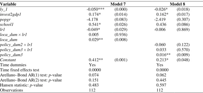
To clarify the impact of the real exchange rates on growth, I investigate further whether the effect of RER differs with the province’s location (coastal versus inland) or with the policy preference level. In other words: Does the real exchange rate have the same impact on growth in coastal provinces as in inland ones? Does it have the same impact in provinces with ‘high’ as in those with ‘low’ policy preference levels? To answer these questions, I introduce three interaction terms into the growth regressions (see Table 5). In Model 7, loca_dum × lr1 is the interaction term of RER and the location dummy. In Model 8, policy_dum2 × lr1 and policy_dum3 × lr1 are the respective interaction terms of RER and the two dummies for policy preference level. In both models, the nonsignificance of the interaction terms indicates that there is no meaningful difference between these two groups of provinces in terms of how RER affects growth. Moreover, introducing these interaction variables does not change the sign of the real exchange rate and has little effect on its significance: the impact of an appreciation of the RER remains positive in both models and is significant in Model 7.
Table 5. Panel evidence for effect of RER on growth (system-GMM with interaction terms)
Variable Model 7 Model 8
ly_1 -0.050*** (0.000) -0.026* (0.018) invest2gdp1 0.174* (0.014) 0.162* (0.017) popgr -4.178 (0.083) -2.419 (0.307) school1 0.541* (0.026) 0.436 (0.086) lr1 -0.049* (0.029) -0.006 (0.869) loca_dum × lr1 0.005 (0.936) loca_dum 0.029** (0.008) policy_dum2 × lr1 -0.060 (0.122) policy_dum3 × lr1 0.033 (0.570) policy_dum3 0.016** (0.009) Constant 0.412** (0.001) 0.213* (0.048)
Time dummies Yes Yes
Time fixed effects test 0.0000 0.0000
Arellano–Bond AR(1) test: p-value 0.074 0.062 Arellano–Bond AR(2) test: p-value 0.151 0.445
Hansen statistic: p-value 0.483 0.597
Observations 112 112
Notes: See notes to Table 4. policy_dum2 is not included in Model 8 because its coefficients are not significant in
previous regressions (see Table 4).
5 Discussion
Several channels of transmission could explain the impact of the real exchange rate on economic growth. For example, the size of a country’s tradable sector was proposed by Rodrik (2008), who argued that the tradable sector suffers more than the nontradable sector from institutional weakness and/or market failure. If this is true then currency undervaluation would have the effect of shifting resources toward industry and would thus constitute a subsidy policy for spurring tradables and generating more rapid growth.
There is no doubt that price distortions exist in China’s industries and tradable sectors. Yet the changes observed during its transition from a planned to a market economy cannot be explained solely by the undersized tradable sector that characterizes developing countries. After all, some nontradable sectors in China, including agriculture and service, have suffered from
price distortions and have been also undersized. During the post-1978 reforms, the government eliminated many of the distortions that it had previously imposed on the price system. Before China’s economic opening, the priority given to industrial development (and the need to ensure a source of budget revenues) led the socialist government to set high prices for industrial production; in relative terms, then, agricultural products and services were undervalued. The gradual opening of the economy to competition and international trade—along with the elimination of government price controls—decreased the price of tradable goods relative to the price of services and agricultural products (Naughton, 2007, pp. 154–155).
While reducing price distortion, the increase of prices in nontradable sectors can facilitate economic growth in three ways. First, an RER appreciation will reallocate resources between the tradable and the nontradable sectors. Therefore, it could not only encourage monopolistic (or collusively oligopolistic) firms to improve their technical efficiency but also spur a more balanced economic growth in the medium and long term. Second, an increasing RER generates a wealth effect by enriching the agricultural and service sectors—or the provinces that specialize in these sectors—and increasing the demand and consumption of tradable and nontradable goods both. Third, but no less important, is that an increase in the price of nontradable goods would induce a rise in the real remuneration of workers and hence improvement in ‘X-efficiency’ proposed by Leibenstein, (1966).
6 Concluding remarks
This paper uses the robust system-GMM estimator to implement a dynamic panel estimation of an informal growth equation applied to 28 Chinese provinces. In most cases I find conditional convergence among the coastal provinces and also among the inland provinces, even though there is no conditional convergence between the two groups of provinces. Consistently with the literature, I find that geographic location and level of policy preference have an impact on provincial performance and on convergence at the national level. Finally, an appreciation of the real exchange rate has a positive influence on provincial economic growth.
Further studies and evidence are needed to shed more light on the mechanisms—such as domestic savings and investment—through which the real exchange rate affects economic growth (cf. Bresser-Pereira, 2006; Gala, 2008). Such studies would help to clarify the effectiveness of a country’s RER policy as a tool for improving the structure of industry specialization and thereby ensuring sustainable growth.
References
Acemoglu, D., Johnson, S. Robinson, J. and Thaicharoen, Y. (2003). 'Institutional causes, macroeconomic symptoms: volatility, crises and growth', Journal of Monetary Economics, 50, pp. 49–123.
ADB (2010), 'Asian Development Bank outlook 2010: Macroeconomic management beyond the crisis', Technical report, Asian Development Bank, Philippines.
Aghion, P., Bacchetta, P., Rancière, R. and Rogoff, K. (2009). 'The real exchange rate and economic growth', Journal of Monetary Economics 56 (4), pp.494-513.
Arellano, M. and Bover, O. (1995). 'Another look at the instrumental variable estimation of error-components models', Journal of Econometrics 68 (1), pp. 29-51.
Barro, R. J. (1991). 'Economic growth in a cross section of countries', The Quarterly Journal of Economics 106(2), pp. 407-43.
Barro, R. J. and Lee, J.-W. (2001). 'International data on educational attainment: updates and implications', Oxford Economic Papers 53(3), pp. 541-63.
Barro, R. J. and Sala-i-Martin, X. (2004). Economic Growth, MIT Press, Cambridge MA.
Benaroya, F. and Janci, D. (1999). 'Measuring exchange rates misalignments with purchasing power parity estimates', in Collignon, S., Pisani-Ferry J. and Park, Y. C. (ed.), Exchange Rate Policies in Emerging Asian Countries, Routledge, New York.
Béreau, S. Villavicencio, A. L. and Mignon, V. (2009). 'Currency misalignments and growth: a new look using nonlinear panel data methods', CEPII Working Papers No. 2009-17, CEPII research center.
Berg, A. and Miao, Y. (2010). 'The real exchange rate and growth revisited: the Washington consensus strikes back? ', IMF Working Papers 10/58, International Monetary Fund.
Blundell, R. and Bond, S. (1998). 'Initial conditions and moment restrictions in dynamic panel data models', Journal of Econometrics 87(1), pp. 115 - 143.
Bond, S. Hoeffler, A. and Temple, J. (2001). 'GMM estimation of empirical growth models', Economics Papers 2001-W21, Economics Group, Nuffield College, University of Oxford.
Bresser-Pereira, L. C. (2006). 'Exchange rate, fix, float or manage it?', Preface to Vernengo, M. (ed.), Financial Integration or Dollarization: No Panacea, Cheltenham, Edward Elgar.
Bussière, M. and Fratzscher, M. (2008). 'Financial openness and growth: short-run gain, long-run pain?', Review of International Economics 16(1), pp. 69-95.
Caselli, F. Esquivel, G. and Lefort, F. (1996). 'Reopening the convergence debate: A new look at cross-country growth empirics', Journal of Economic Growth 1, pp. 363-389.
Chen, J. and Fleisher, B. M. (1996). 'Regional income inequality and economic growth in China', Journal of Comparative Economics 22(2), pp. 141-164.
Chen, M. and Zheng, Y. (2008). 'China's regional disparity and its policy responses', China and World Economy 16(4), pp. 16-32.
Cottani, J. A. Cavallo, D. F. and Khan, M. S. (1990). 'Real exchange rate behavior and economic performance in LDCs', Economic Development and Cultural Change 39(1), pp. 61-76.
Démurger, S. Sachs, J. D. Woo, W. T. BAO, S. and Chang, G. (2002). 'The relative contributions of location and preferential policies in China's regional development: being in the right place and having the right incentives', China Economic Review 13(4), pp. 444-465.
Devereux, J. and Connolly, M. (1996). 'Commercial policy, the terms of trade and the real exchange rate revisited', Journal of Development Economics 50(1), pp. 81 - 99.
Ding, S. and Knight, J. (2008). 'Why has China grown so fast? The role of structural change', Economics Series Working Papers 415, University of Oxford, Department of Economics.
Ding, S. and Knight, J. (2009). 'Can the augmented Solow model explain China's remarkable economic growth? A cross-country panel data analysis', Journal of Comparative Economics 37(3), pp. 432 - 452.
Dollar, D. (1992). 'Outward-oriented developing economies really do grow more rapidly: evidence from 95 LDCs, 1976-1985', Economic Development and Cultural Change 40(3), pp. 523-44.
Dufrénot, G. Mignon, V. and Tsangarides, C. (2010). 'The trade-growth nexus in the developing countries: a quantile regression approach', Review of World Economics (Weltwirtschaftliches Archiv) 146(4), pp. 731-761. Edwards, S. (1990). Real exchange rates in developing countries: concepts and measurement, in Grennes, T. J. (ed.),
'International Financial Markets and Agricultural Trade', Westview Press, Boulder, Colo., pp. 56-108.
Eichengreen, B. (2007). 'The real exchange rate and economic growth', Working Paper No.4, Commission on Growth and Development.
Fleisher, B. M. and Chen, J. (1997). 'The coast-noncoast income gap, productivity, and regional economic policy in China', Journal of Comparative Economics 25(2), pp. 220-236.
Fleisher, B. Li, H. and Zhao, M. Q. (2010). 'Human capital, economic growth, and regional inequality in China', Journal of Development Economics 92(2), pp. 215-231.
Gala, P. (2008). 'Real exchange rate levels and economic development: theoretical analysis and econometric evidence', Cambridge Journal of Economics 32(2), pp. 273-288.
Garroway, C. Hacibedel, B. Reisen, H. and Turkisch, E. (2010). 'The renminbi and poor-country growth', OECD Development Centre Working Paper No 292, OECD Publishing.
Gemmell, N. (1996). 'Evaluating the impacts of human capital stocks and accumulation on economic growth: some new evidence', Oxford Bulletin of Economics and Statistics 58(1), pp. 9-28.
Ghura, D. and Grennes, T. J. (1993). 'The real exchange rate and macroeconomic performance in Sub-Saharan Africa', Journal of Development Economics 42(1), pp. 155-174.
Goldfajn, I. and Valdes, R. O. (1996). 'The aftermath of appreciations', NBER Working Paper No. 5650, Cambridge, MA: NBER.
Gonzalez, A. Trasvirta, T. and Dijk, D. v. (2005). 'Panel smooth transition regression models', Working Paper Series in Economics and Finance 604, Stockholm School of Economics.
Guillaumont Jeanneney, S. and Hua, P. (2001). 'How does real exchange rate influence income inequality between urban and rural areas in China?', Journal of Development Economics 64(2), pp. 529-545.
Guillaumont Jeanneney, S. and Hua, P. (2008). 'Appreciation of the renminbi and urban-rural income disparity in China', Revue d'éonomie du développement 22(5), pp. 67-92.
Hao, C. (2006). 'Development of financial intermediation and economic growth: The Chinese experience', China Economic Review 17(4), pp. 347-362.
Hausman, J. A. (1978). 'Specification Tests in Econometrics', Econometrica 46 (6), pp. 1251–1271.
Herrerias, M. J. and Orts, V. (2011). 'The driving forces behind China's growth', The Economics of Transition 19(1), pp. 79-124.
Heshmati, A. (2004). 'Continental and sub-continental income inequality', IZA Discussion Papers 1271, Institute for the Study of Labor (IZA).
Holz, C. A. (2006). 'China's reform period economic growth: how reliable are Angus Maddison’s estimates?', Review of Income and Wealth 52(1), pp. 85-119.
Hu, A. Wang, S. and Kang, X. (1995). China regional disparity report, Liaoning People’s press, Shenyang, China. Hurlin, C. and Mignon, V. (2005). 'Une synthèse des tests de racine unitaire sur données de panel', Economie and
prévision 3(169-170-171), pp. 253-294.
Im, Kyung-So, Pesaran, Hashem and Shin, Yongcheol (2003). 'Testing for Unit Roots in Heterogeneous panel', Journal of Econometrics, 115(1), pp. 53-74.
Islam, N. (1995). 'Growth empirics: a panel data approach', The Quarterly Journal of Economics 110(4), pp. 1127-70.
Jones, C. I. (1997). 'On the evolution of the world income distribution', Journal of Economic Perspectives 11(3), pp. 19-36.
Leibenstein, H. (1966). 'Allocative efficiency vs. "X-efficiency"', The American Economic Review 56(3), pp. 392-415..
Levine, R. and Renelt, D. (1992). 'A sensitivity analysis of cross-country growth regressions', American Economic Review 82(4), pp. 942-63.
Levy-Yeyati, E. and Sturzenegger, F. (2003). 'To float or to fix: evidence on the impact of exchange rate regimes on growth', The American Economic Review 93(4), pp. 1173-1193.
Li, H. Liu, Z. and Rebelo, I. (1998). 'Testing the neoclassical theory of economic growth: evidence from Chinese provinces', Economic Change and Restructuring 31(2-3), pp. 117-32.
Liu, Z. (2008). 'Foreign direct investment and technology spillovers: theory and evidence', Journal of Development Economics 85(1-2), pp. 176-193.
Loayza, N. Fajnzylber, P. and Calderón, C. (2004). 'Economic growth in Latin America and the Caribbean: stylized facts, explanations, and forecasts', Working Papers Central Bank of Chile 265, Central Bank of Chile.
Lucas, R. J. (1988). 'On the mechanics of economic development', Journal of Monetary Economics 22(1), pp. 3-42. Maasoumi, E. and Wang, L. (2008). 'Economic reform, growth and convergence in China', Econometrics Journal
11(1), pp. 128-154.
Mankiw, N. G. Romer, D. and Weil, D. N. (1992). 'A contribution to the empirics of economic growth', The Quarterly Journal of Economics 107(2), pp. 407-37.
Montiel, P. J. and Hinkle, L. (1999). 'An overview', in Hinkle, L. and Montiel, P. J. (ed.), Exchange Rate Misalignment: Concepts and Measurement for Developing Countries, New York: Oxford University Press. NDRC [National Development and Reform Commission] (2010). The Outline of the Eleventh Five-year Plan for
National Economic and Social Development of the People’s Republic of China. Naughton, B. (2007). The Chinese Economy: Transitions and Growth, The MIT Press.
Nickell, S. J. (1981). 'Biases in dynamic models with fixed effects', Econometrica 49(6), pp. 1417-26.
Pedroni, P. and Yao, J. Y. (2006). 'Regional income divergence in China', Journal of Asian Economics 17(2), pp. 294-315.
Quah, D. (1993). 'Galton's fallacy and tests of the convergence hypothesis', The Scandinavian Journal of Economics 95(4), pp. 427-443.
Quah, D. (1997). ' Empirics for growth and distribution: stratification, polarization, and convergence clubs', Journal of Economic Growth 2(1), pp. 27-59.
Rawski, T. G. (2001). 'What is happening to China's GDP statistics?', China Economic Review 12(4), pp. 347-354. Razin, O. and Collins, S. M. (1997). 'Real exchange rate misalignments and growth' NBER Working Paper No. 6174,
Cambridge, MA: NBER.
Rodrik, D., 2008. The real exchange rate and economic growth. Brookings Papers on Economic Activity, Fall, pp. 365-412.
Rodrik, D. (2010). 'Making room for China in the world economy', American Economic Review 100(2), pp. 89-93. Romer, P. M. (1989). 'Human capital and growth: theory and evidence', NBER Working Paper No. 3173,
Cambridge, MA: NBER.
Roodman, D. (2003). 'XTABOND2: Stata module to extend xtabond dynamic panel data estimator', Statistical Software Components, Boston College Department of Economics.
Salter, W. E. G. (1959). 'Internal and external balance: the role of price and expenditure effects', The Economic Record 35(71), pp. 226-238.
Solow, R. (1956). 'A contribution to the theory of economic growth', The Quarterly Journal of Economics 70(1), pp. 65-94.
Temple, J. (1999). 'The new growth evidence', Journal of Economic Literature 37(1), pp. 112-156.
Wang, S., and Hu, A. (1999). 'The political economy of uneven development: the case of China', Armonk, NY: M.E. Sharpe.
Woo, W. T. (1999). 'The real reasons for China's growth', The China Journal 41, pp. 115-137.
Woo, W. T. (2009). 'China in the current global economic crisis', Testimony before the U.S.-China Economic and Security Commission.
Xu, L. C. and Zou, H.-F. (2000). 'Explaining the changes of income distribution in China', China Economic Review 11(2), pp. 149-170.
Yang, Dennis Tao (2002). 'What has caused regional inequality in China?', China Economic Review 13(4), pp. 331-334.
Yao, S. (2006). 'On economic growth, FDI and exports in China', Applied Economics 38(3), pp. 339-351.
Zheng, J. Hu, A. and Bigsten, A. (2009). 'Potential output in a rapidly developing economy: the case of China and a comparison with the United States and the European Union', Review (Jul), pp. 317-342.
Data Appendix
PPI: The missing values from 1992 to 1996 for certain provinces correspond to Shanxi
(1992–1994), Jilin (1992–1996), Fujian (1992–1994), Hubei (1992–1994, 1996), Guangdong (1992–1996), Guizhou (1992–1993), Gansu (1992), and Ningxia (1992–1996). The missing values were replaced with the country PPI for the corresponding year (as extracted from the CSY of 2000, 2001, and 2002).
Trade openness:
For the period 2005–2008, the values of imports (resp., exports) are calculated in terms of their provinces of destination in China where the imported commodities are consumed, used or transported to (resp., their provinces of origin in China where the exported commodities are produced or originally delivered); the only alternative statistics available at the provincial level for this period are based on the location (i.e. province) where import or export corporations are situated, i.e., where they have applied and have registered at the Chinese Customs. The calculation method of foreign trade is not specified for the years prior to 2005.
Table A1. Definition and sources of variables
Variable Definition Sources gdp_cur Current-price gross domestic product (100 million yuan,
annual)
CCS, 2010 CSA
pop_end Year-end population (×10,000, annual) 2009 CPESY
g Growth rate of real GDP per capita (annual, PA) CCS, 2010 CSA, 2009 CPESY
ly_1 Real GDP per capital (yuan, BP) CCS, 2010 CSA,
2009 CPESY
Invest2gdp1 Ratio of gross capital formation to GDP (in current price) (annual, PA)
CCS, 2010 CSA
Invest2gdp2 Ratio of fixed capital to GDP (in current price) (annual, PA)
CCS, 2010 CSA
popgr Natural growth rate of the population (annual, PA) CCS, 1997 CSY
school1 Ratio of gross secondary school enrollment to total population (annual, BP)
CCS, 2006–2009 CSY
school2 Ratio of population with at least a senior high school education to total population (annual, BP)
1997–2000 CSY, 2002–2009 CSY, 1993–1996 CPSY, 2002 CPSY
open Ratio of combined imports and exports to GDP (in current price) (annual, PA)
CCS, 2010 CSA
fdi2gdp Ratio of foreign direct investment to GDP (in current price) (annual, PA)
CCS, 2010 CSA
fdi2invest Ratio of FDI to fixed capital formation (in current price) (annual, PA)
CCS, 2010 CSA
lr1 Real exchange rate: ln (PPI ÷ CPI) (annual, BP) CCS
lr2 Real exchange rate: ln[1 ÷ CPI] (annual, BP) CCS
loca_dum Location dummy Ding and Knight (2008)
policy_var Policy preference level Pedroni andYao (2006)
Key: BP = beginning of each five-year period; CCS = China Compendium of Statistics 1949–2008;
CPESY = China Population and Employment Statistics Yearbook; CPSY = China Population Statistical Yearbook; CSA = China Statistical Abstract; CSY = China Statistical Yearbook; PA = period average (over five years).