Flight guidance along 3D+T trajectories and space indexed traffic management

(1)

T

H

È

S

E

En vue de l’obtention du

DOCTORAT DE L’UNIVERSITÉ DE TOULOUSE

Délivré par : l’Université Toulouse 3 Paul Sabatier (UT3 Paul Sabatier) Présentée et soutenue par :

M

ASTURA

AB WAHID

le 8/12/2015 Titre:

FLIGHT GUIDANCE ALONG 3D+T TRAJECTORIES AND SPACE INDEXED TRAFFIC MANAGEMENT

École doctorale er discipline ou spécialité

ED MITT : Domaine Mathématiques : Mathématiques appliquées Unité de recherche :

Laboratoire de Mathématiques Appliquées, Informatique et Automatique pour l'Aérien (MAIAA), ENAC

Directeurs de Thèse :

FÉLIX MORA-CAMINO (Directeur) ANTOINE DROUIN (Co-Directeur)

Jury :

FRANCISCO JAVIER SAEZ NIETO Rapporteur DAVID ZAMMIT-MANGION Rapporteur BENOÎT DACRE-WRIGHT Examinateur CHRISTIAN BÈS Examinateur

(2)

(3)

(4)

(5)

ACKNOWLEDGMENT

Firstly I would like to give my gratitude to the Ministry of Education Malaysia and Universiti Teknologi Malaysia (UTM) for giving me a scholarship to pursue my studies in France for both Master and PhD degrees from 2010 to 2015. Secondly, I am thankful to my Supervisor Prof. Dr. Felix Mora-Camino for accepting me in MAIAA laboratory as his PhD student and for being attentive with me. I have learned a lot under his guidance and his many ideas have helped me to complete this thesis. Thank you. Thirdly, I want to thank my second supervisor, Dr. Antoine Drouin who helped me with the numerical simulation part. Also, I want to thank my colleague, now Dr. Hakim Bouadi, who has given me assistance during my first year of internship. I found his thesis to be very useful as a basis for my own research. Also, not forgetting the important people in my life, my husband, both my parents and in-laws and my sisters who have given me moral support, for that I thank you. Last but not least, I would like to give my sincerest gratitude to all my friends here in this lab, in Toulouse and Malaysia. The discussion that we had either about the research or other things have given me ideas, helped me find solutions and also helped me unwind during my PhD years. Thank you All.

(6)

(7)

To my loving husband Suffyan… To my supportive parents Ab Wahid, Norbiha…

(8)

(9)

ABSTRACT

With the increase in air traffic, surely a question of flight efficiency (delays), environment impact and safety arise. This calls for improvements in accuracy of spatial and temporal trajectory tracking. The first main objective of this thesis is to contribute to the synthesis of a space-indexed nonlinear guidance control law for transportation aircraft presenting enhanced tracking performances and to explore the performances and feasibility of a flight guidance control law which is developed based on a space-indexed reference to track a 3D+T reference trajectory using nonlinear dynamic inversion control. The proposed guidance control law present reduced tracking errors and able to meet more easily overfly time constraints. Before presenting the main approaches for the design of the 3D+T guidance control laws; the modern flight guidance and flight dynamics of transportation aircraft, including explicitly wind components are first introduced. Then, a description of the current and modern air traffic organization including the organization of air traffic in high density flow will be shown and this will lead to a description of the Airstreams concept. This proposed concept is to organize main traffic flows in congested airspace along airstreams which are characterized by a three dimensional (3D) common reference track (ASRT). Finally, a scenario to perform basic maneuvers inside the airstream following a 3D+T trajectory using a common space-indexed will be developed and will be used to illustrate the traffic management along an airstream. Keywords: Airstreams, 3D+T trajectory tracking, flight guidance, space-indexed nonlinear control.

(10)

(11)

RESUME

Avec la forte augmentation actuelle et future du trafic aérien, les questions relatives à la capacité, la sécurité et les effets environnementaux du transport aérien vont se poser de façon chaque fois plus critique. L’objectif général de cette thèse est de contribuer à l´amélioration de l’opération et de l´organisation du trafic aérien dans cette perspective de croissance.

Le premier objectif spécifique de cette thèse est de faire la synthèse d'une loi de commande permettant aux avions de transport de suivre avec précision une trajectoire 3D+T.

Le deuxième objectif spécifique de cette thèse est d´introduire une organisation particulière des corridors aériens, les airstreams, compatible avec la loi de guidage développée et permettant d´utiliser au mieux la capacité du corridor.

Ainsi dans une première étape est introduite la dynamique de guidage des avions de transport, ainsi que les systèmes de guidage et de gestion du vol des avions modernes. Ensuite les principaux éléments de l´organisation de la gestion et du contrôle du trafic aérien sont introduits. La loi de guidage 3D+T est développée, simulée et ses performances sont analysées. L´étude d´une manœuvré de changement de voie dans un airstream est alors menée et mise en œuvre dans le cadre de la gestion du trafic à l’intérieur de celui-ci. Finalement les conclusions et perspectives de cette étude sont présentées.

Mots-clés: Airstream, suivi de trajectoire 3D+T, guidage du vol, commande non linéaire indexées espace.

(12)

(13)

LIST OF FIGURES

Figure 2.1: Earth Centered Inertial Frame and Earth-Ceterd Earth-Fixed

Frame [Fr.mathworks.com, 2015] ... 10

Figure 2.2: Local Earth Frame ... 11

Figure 2.3: Aircraft body axis frame ... 11

Figure 2.4: Wind axis (w), Stability axis (s) and Body axis (b) ... 12

Figure 2.5: Transformation from inertial frame to the body frame [Mora-Camino, 2014] ... 13

Figure 2.6: Relative wind ... 15

Figure 2.7: Angles relating the orientation of the airspeed Va with respect to Local Earth and Body frame respectively ... 15

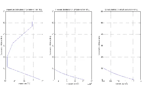
Figure 2.8: International Standard Atmosphere ... 20

Figure 2.9: International Standard Atmosphere ... 20

Figure 2.10: Aerodynamic Forces ... 22

Figure 2.11: Global view of flight equations [Mora-Camino, 2014] ... 27

Figure 3.1: Overall classical structure of flight control systems [Mora-Camino, 2014] ... 32

Figure 3.2: Flight Management System (FMS) Block Diagram [Collinson, 2011]... 33

Figure 3.3: Multifunction Control Display Unit (MCDU) [Wikipedia, 2015d] ... 34

Figure 3.4: Example of lateral (track) flight plan ... 35

Figure 3.5: Vertical Flight Profile [Collinson, 2011] ... 37

Figure 3.6: Primary Flight Display (PFD) – Boeing term[Wikipedia, 2015c] ... 40 Figure 3.7: Navigation Display (ND) – Boeing term. Indicates the aircraft track, waypoints / pseudo-waypoints and other navigation information

(18)

Figure 3.9: Example architecture of FMS/FGS in A320 [Bouadi, 2013] ... 43

Figure 3.10: GPWS thresholds modes with the aural and visual warning[GPS, 2001] ... 46

Figure 4.1 : General Airspace Classification [FAA, 2013] ... 53

Figure 4.2: Example of routes segregation and convergent of traffic at the entry [EUROCONTROL, 2014] ... 56

Figure 4.3: Good design practice proposed by ICAO for departure (DEP) and arrival (ARR) vertical constraints [EUROCONTROL, 2010] ... 56

Figure 4.4: From classical to RNAV operation [Todorov, 2009] ... 58

Figure 4.5: RNP-X definition means that navigation system must be able to calculate its position to within a circle with a radius of X nautical miles. The 2 x RNP containment limit represents the level of assurance of the navigation performance with a 99.999% percent probability per flight hour ... 59

Figure 4.6 : Navigation specification for RNP and RNAV ... 59

Figure 4.7: Corresponding RNP designation to the TSE value [AIRBUS, 2009] ... 60

Figure 4.8: Definition of NSE, FTE and PDE [AIRBUS, 2009] ... 60

Figure 4.9: US expected evolution of traffic management [Barraci, 2010] ... 62

Figure 4.10: Overview of the traffic separation system ... 63

Figure 4.11 : The Aircraft Protection Zone ... 63

Figure 4.12: Countries that have fully/partially implemented FRA as of end 2014 [EUROCONTROL, 2015c] ... 65

Figure 4.13: Example of continuous descent approach (CDA) and continuous climb operation (CCO) ... 68

Figure 5.1: Nominal design of Corridor Building block [Yousefi et al., 2010] ... 74

Figure 5.2: Separation Requirements ... 75

Figure 5.3: Speed-Dependent Track – designated by nominal Mach number [Wing et al., 2008] ... 75

Figure 5.4: Speed independent track[Wing et al., 2008] ... 76

Figure 5.5: Conflict resolution: Speed of aircraft A is 250m/s while aircraft B is 230 m/s. Both aircraft make a slight left and right turn to achieve required separation. ... 78

(19)

Figure 5.8 : The local airstream frame at point S ... 82

Figure 5.9 : Reference point in cross section plane... 83

Figure 5.10: Track speed along the ASRT ... 85

Figure 6.1: Organization of traffic around a common reference track (ASRT) ... 94

Figure 6.2: Projection of airspeed along ASRT ... 94

Figure 6.3: Piloting and Guidance Dynamics ... 96

Figure 6.4: Aircraft following the center of a moving slot. ... 100

Figure 6.5: Simulation settings... 109

Figure 6.6: Perturbation rejection property of the guidance law... 110

Figure 6.7: Wind gust rejection during a constant velocity horizontal trajectory... 111

Figure 6.8: Tracking of a 3D+T trajectory consisting in a change of velocity at constant altitude and heading ... 112

Figure 6.9: Tracking of a 3D+T trajectory consisting in a change of altitude at constant velocity ... 112

Figure 6.10: Tracking of a 3D+T lane change trajectory ... 113

Figure 6.11: Pertubation rejection of a traditional time-indexed NLI guidance law ... 113

Figure 6.12: Pertubation rejection of the space-indexed NLI guidance law ... 113

Figure 7.1: Non-invertibility situations ... 128

Figure 7.2: Non-invertibility situations in cruise ... 128

Figure 8.1: Standard shift maneuver in an airstream ... 134

Figure 8.2: Standard shift maneuver between lanes in an ASRT... 136

Figure 8.3: Example of transient (blue) flights and assigned (green) flight along an ASRT ... 140

(20)

(21)

LIST OF TABLES

Table 2.1: ISA assumes the conditions at mean sea level (MSL) ... 19

Table 2.2: Variation of TLR according to altitude ... 19

Table 3.1: Lateral Guidance Modes [Tribble et al., 2002] ... 41

Table 3.2: Vertical Guidance Modes [Tribble et al., 2002] ... 42

Table 4.1: Separation Minima ... 54

Table 4.2: Horizontal Separation Minima for non-radar area between two aircraft ... 55

Table 7.1: Attitude Performance of inertial navigation systems (INS) with GPS-updating [Schwarz, 1996] ... 118

Table 7.2: Velocity performance of inertial navigation systems (INS) with GPS-updating [Schwarz, 1996] ... 118

Table 7.3: ICAO GNSS Signal-in-Space Performance Requirements [Spitzer, 2001] ... 119

Table 7.4: Actual GNSS Signal-in-Space Performance [Spitzer, 2001] ... 119

Table 7.5: A typical air-data computer accuracy requirements [Kayton and Fried, 1997] ... 119

Table 8.1: Initial situation in ARST ... 144

Table 8.2: First ranking between transient flights ... 144

Table 8.3: Final proposed assignment and performance ... 145

Table B.0.1: Aircraft Configuration ... 175

(22)

(23)

NOMENCLATURE

3D+T 3 Dimensional Plus Time

A/THR Auto-Throttle

AP Auto-Pilot

ASAS Airborne Separation Assurance System ASRT Airstream Reference Track

ATC Air Traffic Control ATC Air Traffic Controller

ATFM Air Traffic Flow And Capacity Management ATM Air Traffic Management

ATS Air Traffic Services

CNS/ATM Communications, Navigation, And Surveillance/Air Traffic Management

ECEF Earth-Centered Earth-Fixed ECI Earth-Centered-Inertial Axis FAA Federal Aviation Association FANS Future Air Navigation Systems

FB Body-Reference Frame

FCU Flight Control Unit FGS Flight Guidance Systems FMS Flight Management Systems Fs Stability Reference Frame

FW Wind Reference Frame

GNSS Global Navigation Satellite Systems

(24)

MCDU Multifunction Control Display Unit

ND Navigational Display

NEXTGEN Next Generation Air Transportation System PBN Performance Based Navigations

PBO Performance Based Operations PDF Primary Flight Display

RNAV Area Navigation

RNP Required Navigation Performance SESAR Single European Sky Atm Research TBO Trajectory Based Operations

TCAS Traffic Collision Avoidance System TLR Temperature Lapse Rate

TMA Terminal Maneuvering Area

x Aircraft Inertial Velocity In X-Direction y _{Aircraft Inertial Velocity In Y-Direction} z Aircraft Inertial Velocity In Z-Direction

c Mean Aerodynamic Chord

i

 _{Gain For}i{ , , }x y z

si

 _{Space Natural Frequency For}i{ , , }x y z

ni

 _{Time Natural Frequency For}i{ , , }x y z * f j m Merging Trajectory  )

( Rate Of The Concerned Variables

 Angular Rate

 Yaw Angle

 Pitch Angle

 Roll Angle

 Flight Path Angle

 Heading Angle

 Angle Of Attack

 Side Slip Angle

(25)

 Azimuth Angle  Tracking Error a Air Density e Elevator Deflection r Rudder Deflection TH Thrust Command

CD Aerodynamic Drag Coefficient

CL Aerodynamic Lift Coefficient

CLM Yawing Moment Coefficient

CM Pitching Moment Coefficient

CN Rolling Moment Coefficient

CY Aerodynamic Side Force Coefficient

D Aerodynamic Drag Force

F Forces

g Gravity

Ja Set Of Assigned Aircraft

JT Set Of Non-Assigned/Transient Aircraft

L Longitude Angle

L Aerodynamic Lift Force

M Latitude Angle

m Mass

Mj Set Of Conflict Free Trajectories

p Roll Rate

q Pitch Rate

R Distance To The Center Of The Earth

r Yaw Rate

S Area Of The Wing

s Curvilinear Abscissa

t Time

u Aircraft Body Velocity In X-Direction

(26)

w Aircraft Body Velocity In Z-Direction

W Wind Components In Body Frame

w Wind Components In Body Frame

YF Aerodynamic Side Force

X Direction Along X-Axis

Y Direction Along Y-Axis

Z Direction Along Z-Axis

SUBSCRIPT

W Components Wind Axis

b Components Body Axis

E Components Local Earth Frame S Components Stability Frame

g Gravitational Forces

T Thrust Forces

a Components Of Aerodynamic Forces s Position On The Curvilinear Abscissa S ASRT Along Airstream Reference Track

(27)

CHAPTER 1

(28)

(29)

Chapter 1: General Introduction

It is forecasted that by the year 2035, both Europe and United States will be handling up to 1.4 billion air travellers/passengers [IATA, 2014], [STATFOR, 2013] and consequencely increasing the air traffic volume. With the increase in air traffic, inevitably questions about flight efficiency (delays), impacts on the environment and safety will arise. To face these issues, improvements in accuracy and reliability of spatial and temporal trajectory tracking by transportation aircraft are expected. Already in 1993, the Special Committee on Future Air Navigation Systems (FANS) provided a recommendation called Communications, Navigation, and Surveillance/Air Traffic Management (CNS/ATM) for the design of new on-board systems. These CNS/ATM systems were to ease the handling and transfer of information, improve aircraft surveillance using latest technology (Automatic Dependent Surveillance Systems) and increase aircraft navigational accuracy (Area Navigation (RNAV) and Global Navigation Satellite Systems (GNSS)).

The demand from CNS/ATM to modernize the future air navigation resulted in worldwide research and more recently in two pioneer projects: the Single European Sky ATM Research (SESAR) project and the american Next Generation Air Transportation System (NextGen) project. The main improvements expected from Future Air Navigation systems were:

- Strategic data link services for sharing of information;

- Negotiation of planning constraints between ATC (Air Traffic Control) and aircraft in order to ensure planning consistency;

- The use of the 3D+T aircraft trajectory information in the Flight Management System for ATC operations.

An exigency of future ATM systems is to have a safe, efficient and predictable flight through a continuous accurate knowledge of the aircraft position [Christopher et al., 2013, De Prins et al., 2013]. Then flight plans should become 3D+T (3 space dimensions and time) objects allowing what is called today Trajectory Based

(30)

traffic in restrained space and time. Also, TBO integrates advanced Flight Management System (FMS) capabilities with ground automation to manage aircraft trajectories in latitude, longitude, altitude, and time in order to dynamically adapt the aircraft flight path to new ATC directives. As a consequence, TBO would allow aircraft to fly safely in high density air flows while adopting efficient trajectories in the context of Free Flight [Kotecha and Hwang, 2009, Ye et al., 2014, Yousefi et al., 2010]. Free Flight and Corridor Flows are some of the research and development projects contribution to TBO [Bowen, 2014, Enea and Porretta, 2012, NextGEN, 2010].

The current air transportation aircraft guidance systems generate in real time corrective actions to maintain the flight trajectory as close as possible to the flight plan or to comply with the spatial or temporal directives issued by ATC. Wind remains one of the main causes for guidance errors and flight inefficiency [Miele, 1990, Psiaki and Park, 1992, Stengel and Psiaki, 1985]. Today the the current navigation systems on board commercial aircraft present a high accuracy and reliability through the fusion of air data, inertial data and satellite information . With classical control techniques, the corresponding guidance errors are still large even with the adoption of time-based guidance control laws [Mulgund and Stengel, 1996]. The recent introduction of space-indexed guidance control laws provides a new perspective for improved tracking performances and enhanced track predictability, even in the presence of wind [Bouadi and Mora-Camino, 2012, Bouadi et al., 2012]. High density air traffic situations will lead to guidance requirements where aircraft are to follow with accuracy a 3D+T trajectory to ensure traffic safety. This leads to the concept of space-indexed control which has been initially developed in 2D+T for vertical guidance in [Bouadi et al., 2012].

Therefore, the first objective of this thesis is to contribute to the synthesis of a space-indexed nonlinear guidance control law for transport aircraft presenting enhanced 3D+T tracking performances.

The second objective of this thesis is to explore the performance and feasibility of a flight guidance control law designed to make the aircraft follow a 3D+T trajectory within a high density traffic corridor. The case of an airstream (introduced

(31)

in Chapter 5) with synchronized slots along lanes and nominal lane change trajectories will be more particularly considered in Chapter 8.

The relevent background, the adopted methodology and the main findings of this research are presented in this report dissertation . The first chapters describe the principal object of this study, i.e. the transportation aircraft and its flight dynamics, then the current technological and methodological environment is introduced either when considering on-board systems or considering air traffic management and control. Current developments and prospective organizations for high density traffic are analyzed. Then a new 3D+T guidance approch is developed and illustrated while its limitations are discussed. Trajectory tracking within an airstream is then considered, showing the interest for this space indexed organization for high density traffic. The detailed chapters organization of the report is as follows:

Chapter Two introduces the flight dynamics of transport aircraft with the main reference frames for wind, forces and motion, with a special interest for guidance dynamics. The evolution of the position of the aircraft, its translational speed, its angular attitude and rotational speed are then expressed through a 12 order nonlinear state representation. The distinction between fast and slow dynamics allows the identification on one side the piloting dynamics and on the other side the guidance dynamics.

Chapter Three describes the main characteristics, modes and functions developed by modern flight guidance systems on board transport aircraft. Then the composition and construction of traditional flight plans by Flight Management Systems (FMS) are described. This flight plan generates the main guidance references used by the flight guidance system unless some ATC directive is received or some guidance protection is activated.

Chapter Four discusses the recent evolution of the air traffic organization towards the future air traffic system. The required Navigation Performances (RNP) from the arrival/approach areas, the Terminal Maneuvering Area (TMA) and the En-Route area are introduced. Then a general presentation of modern traffic management

(32)

Chapter Five introduces first the concept of an air corridor which is envisioned by the United States to absorb in a safe way high density traffic within the Trajectory Based Operations (TBO) concept. Then the concept of Airstream is described, where traffic is distributed on lanes located around a geometric (3D) reference track (Airstream Reference Track-ASRT). In that case traffic on each lane is assigned in a synchronized way along moving slots.

Chapter Six formulates the 3D+T guidance problem around a reference trajectory. The tracking error requirements are given using a space indexed performance which is converted to a time-based tracking error performance. Then a normal nonlinear dynamic inversion is performed to generate the control inputs to be applied to the guidance dynamics. The fast dynamics under the inner loop of the flight control system (auto-pilot) is supposed to behave in a standard way and the design of the pilot law is not considered, concentrating on the design of a generic auto-guidance law.

Chapter Seven analyzes the limitations of the control design approach presented in chapter six. Issues regarding the effect of on-board sensors inaccuracy and parameter errors on the guidance performances are considered. Also potential numerical problems are investigated and the compatibility of this new guidance function with existing guidance systems is discussed.

Chapter Eight introduces the space-indexed parameterization of a 3D+T trajectory performing the transfer from a synchronized lane to another within an airstream. This 3D+T trajectory will serve as reference for aircraft shifting from one lane to another. The management of traffic within an airstream is then considered.

Chapter Nine, the final chapter, gives a general conclusion on the main efforts developed in this research work and concludes whether the objectives are achieved. Finally a general perspective of the work and potential issues to pursue the current research are given.

(33)

CHAPTER 2 TRANSPORTATION AIRCRAFT FLIGHT

DYNAMICS

(34)

(35)

Chapter 2: Transport Aircraft Flight Dynamics

2.1 Introduction

This chapter describes and analyzes the flight dynamics of transport aircraft as we are interested in designing a new guidance system for them. Once reference frames as well as the main relevant variables to describe atmospheric flight are introduced, the flight dynamics equations are established following main principles of mechanics and aerodynamics. These flight equations are shown to be composed on one side, by the fast dynamics related with rotational motion and angular attitude of the aircraft, and on the other side; by the slow dynamics related with the trajectory of the center of gravity of the aircraft. In this thesis we will be more interested with these slow dynamics, as “guidance dynamics” which are directly related with our control objective.

2.2 The reference frames

Reference frames are used to describe the motions of the aircraft with respect to the Earth and the local atmosphere. Earth-Centered Inertial (ECI) is defined to be stationary or moving at a constant velocity. It is inertial. This reference frame is used for the calculation of a satellite’s position and its velocity; also inertial sensors produce measurement relative to the inertial frame. Its origin is located at the center of the Earth. Zi axis points along the nominal axis of rotation. Xi lies in the equatorial

plane and point towards vernal equinox. Yi axis is orthogonal to both axes.

The Earth-Centered Earth-Fixed (ECEF) has the same origin and Z-axis as the ECI frame, but it rotates with the Earth around its North-South axis at an angular rate, IE. It is denoted by (X,Y and Z) This is a basic coordinate frame for navigation

and satellite-based radio navigation systems often used the ECEF coordinates to calculate satellite and aircraft positions.

(36)

Figure 2.1: Earth Centered Inertial Frame and Earth-Ceterd Earth-Fixed Frame [Fr.mathworks.com, 2015]

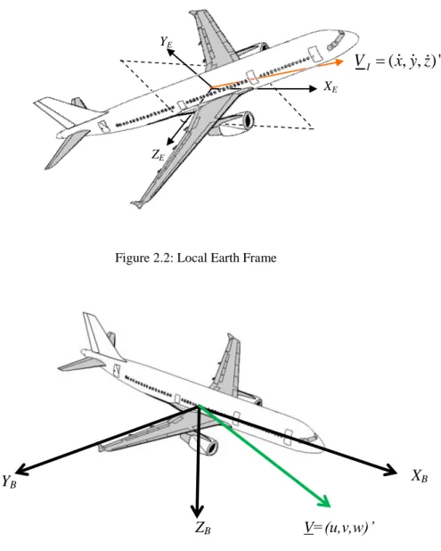
The Local Earth Frame (LEF) shown in figure Figure 2.2 defines the angular altitude of the aircraft with respect to the Earth. The LEF is composed of XE – axis

points towards true north, the ZE-axis is perpendicular towards the ground and the YE

– axis completes the right-handed coordinate systems.

The Body-Axis Frame (FB) shown in Figure 2.3 expresses the speed components

(translational and rotational) with respect to the aircraft main inertial axis. Normally the sensitive axes of the accelerometer sensors are made to coincide with the axes of the moving platform in which the sensors are mounted [Noureldin et al., 2013]. The Xb axis lies in the symmetry plane of the aircraft and points forward. The Zb axis also

lies in the symmetry plane, but points downwards. (It is perpendicular to the Xb axis.)

The Yb axis can again be determined using the right-hand rule. The inertial speed in

the body frame is V=(u,v,w)’

X Y YI XI ZI, Z Equator Pane IE

(37)

Figure 2.2: Local Earth Frame

Figure 2.3: Aircraft body axis frame

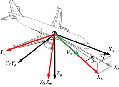
The Stability Reference frame (FS) is a body-carried coordinate system. The Xs

axis is taken as the projection of the velocity vector of the aircraft relative to the air mass, Va into the aircraft plane of symmetry. The angle of attack  is defined as the angle between XS and XB. The ZS axis lies in the plane of symmetry and YS axis is

equal to the YB axis. This frame is considered as an intermediate frame equidistant to

the transformation between the wind frame and the body-fixed axis system. XB ZB YB V=(u,v,w)’ ZE XE YE ( , , ) ' I V  x y z

(38)

is aligned to the ZS axis and the YW axis can now be found using the right-hand rule.

The side slip angle,  is the angle between the Xs and Xw.

Figure 2.4: Wind axis (w), Stability axis (s) and Body axis (b)

2.3 Frame Transformations

According to the physical phenomenon considered it is more convenient to work with one frame than the other. Here the notation for a transformation is RIJ, where I is

the final frame and J is the initial frame.

The transformation from Local Earth Frame to the Body Frame can be done using three Euler’s angles. First we have to rotate over the yaw angle, , around the Z axis. Afterward we rotate over the pitch angle, , about the subsequent Y axis. Finally, the new resulting reference frame is then rotated over the roll angle  - around its X axis. Figure 2.5 shows the transformation. The resulting equation is:

2 1 2 1 ( ) ( ) ( ) ( ) ( ) ( , , ) ( ) ( ) ( ) ( ) ( ) ( ) ( ) ( ) ( ) ( ) ( ) ( ) ( ) ( ) ( ) ( ) ( ) ( ) ( ) ( ) ( ) ( ) ( ) ( ) ( ) ( ) ( ) B v v LB v v L c c c s s R R R R s s c c s s s s c c c s c s c s s c s s s c c c                                            _          _              (2.1)

where ( )c  stands for cos( ) and ( )s  stands for sin( ) . As this rotation matrix is orthonormal, the transformation from the Local Earth Frame to the Body Frame is obtained by inverting the above matrix or taking the transpose.

W X W Y B Y B X B Z W Z   W X W Y B Y B X B Z W Z   XS ZS, YS, Va

(39)

1 2 1 1 ( ) ( ) ( ) ( ) ( ) ( ) ( ) ( ) ( ) ( ) ( ) ( ) ( , , ) ( ) ( ) ( ) ( ) ( ) ( ) ( ) ( ) ( ) ( ) ( ) ( ) ( ) ( ) ( ) ( ) ( ) ( ) ( ) ( ) v v v BL L v L c c s s c c s c s c s s R R R R c s s s s c c c s s s c s c s c c                                                     _          _        (2.2)

In order to avoid angular ambiguities and to comply with transportation aircraft operations the following limits are considered:

-<<, -/2<</2, and -<<

Figure 2.5: Transformation from inertial frame to the body frame [Mora-Camino, 2014]

Another transformation matrix is from the Wind Reference Frame to the Body-Axis Frame. It is used to express the aerodynamic forces and moments in the Body-Axis Frame. The aircraft is first aligned along the wind vector and then rotation through the side slip angle  is performed to reach the Stability Frame before finally a rotation by an angle .

1 1

cos cos sin cos sin

( ) ( ) sin cos 0

cos sin sin cos cos

B WB W R R R                       _{ } _      (2.3)

This rotation matrix is also orthonormal; therefore inversing the matrix to transform back to the Wind Frame is also achieved by transposing this matrix.

(40)

1 1

cos cos sin cos sin

( ) ( ) sin cos cos sin cos

sin 0 cos B BW W R R R                      _  _      (2.4)

For the navigation purposes, we need to transform the LEF to the ECEF frame. The rotation between the ECEF and LEF frames is described by two single axis rotation matrices, and only by the longitude angle, , and latitude angle  as the LEF frame is constrained to have its z-axis to always be perpendicular to the reference ellipsoid. The rotation matrix is given by:

sin( ) cos( ) sin( ) cos( ) cos( ) sin( ) sin( ) cos( ) cos( ) sin( )

cos( ) 0 sin( ) EL R                       _    _      (2.5)

2.4 Aircraft Speeds and Wind Speed

To determine the distance an aircraft has travelled, continuous and accurate information of the ground speed GS should be available to the pilot and other shareholders such as the ATC and the destination airport. An aircraft ground speed GS can be greatly enhanced or diminished by the wind. Therefore the consideration of two speeds: wind speed W and airspeed Va must be considered. Airspeed is the

speed of an aircraft in relation to the surrounding air. Ground speed is the horizontal inertial speed of an aircraft relative to the ground given by:

2 2

GS  x y (2.6)

The components of the wind, W (W W Wx, y, Z) ' in the Local Earth Frame can be represented in the Body Frame using the transformation matrix RLB:

x x y LB y z z w W w R W w W      _               (2.7)

(41)

Figure 2.6: Relative wind

The relationship between the inertial speed VI , wind speed W and air speed Va is

given by:

I a

V V W (2.8)

The inertial speed VI can be expressed both in the Body Frame and the Local Earth

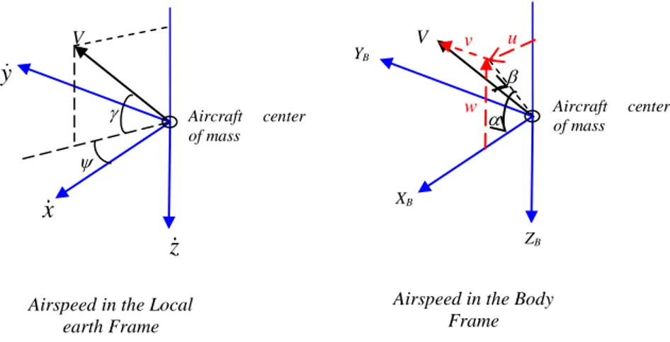
Frame. Before moving into the presentation of each inertial speed VI, understanding

the orientation of the aircraft airspeed Va with respect to Body Frame and the Local

Earth Frame needs to be done (Figure 2.7). The orientation of the aircraft airspeed Va

in the Local Earth Frame can be expressed by flight path angle  and heading angle  while the orientation of the airspeed in the Body Frame can be defined by angle of attack  and side slip angle :

Figure 2.7: Angles relating the orientation of the airspeed Va with respect to Local Earth and Body frame respectively

V

 

Airspeed in the Local earth Frame

V

ZB

 

Airspeed in the Body Frame y XB YB Aircraft center of mass Aircraft center of mass x z u v w W Va VI

(42)

Firstly, considering that there is no wind, from equation 2.8 the inertial speed VI is

the same as the aircraft airspeed Va. Hence the inertial speed in the Local Earth

Frame ( VI ) and in the Body Frame (VB) can be defined from the observation of

Figure 2.7. Then, the aircraft inertial speed in the Local Earth Frame VI is given by:

cos cos cos sin sin a I a a x V V y V z V              _{  } _    _      (2.9)

and the inertial speed in the Body Frame, VB is given by:

cos cos sin cos sin a B a a u V V v V w V              _{  } _         (2.10)

Following a simple trigonometric the airspeed, Va can be given by:

     

2 2 2

a

V  u  v  w or V_a 

     

x 2 y 2 z 2 (2.11)

The angles, flight path angle , heading angle , side slip angle  and angle of attack

(43)

1 sin z V  _        (2.12) 1 2 2 sin y x y  _  _ _  _    (2.13) arctan w u   _{ }   (2.14) arcsin a v V   _ _   (2.15)

Now we will consider when the wind speed is not zero, the inertial speed will not be the same as the airspeed. From equation 2.8 the inertial speed represented in equation 2.9 will become: cos cos cos sin sin a x I a y a z x V W V y V W z V W                  _{  } _{ } _    _          (2.16)

while the airspeed, flight path angle and heading angle will be:





2





2





2 a x y z V  x W  y W  z W (2.17) 1 ( ) sin z Wz V  _         (2.18) 1 2 2 ( ) sin ( ) ( ) x x y y W x W y W  _      _ _ _    (2.19)

Then inertial speed with respect to Body Frame can be found through the conversion from Local Earth Frame to Body Frame. Recalling the transformation matrix in equation 2.1, the inertial speed in the body frame VB can be expressed with the

(44)

cos cos cos sin sin a x LB a y a z u V W v R V W w V W                 _   _             _          (2.21)

and the angle of attack  and sideslip  can be obtained by substituting equation 2.21 into equation 2.14 and 2.15.

2.5 Flight path angle

The flight path angle gives the information to the pilot where the aircraft is heading to in the verticle plane. Flight path angle (angle between the local horizontal plane and the considered speed) can be affected by the wind. From [Mora-Camino, 2014], it was shown that the inertial and air flight path angle (I and a respectively) can be

written as:

arcsin a ( sin cos cos sin cos sin cos cos sin cos ) z I I I V W V V    _             _   (2.22) and

arcsin a ( sin cos cos sin cos sin cos cos sin cos ) a I V V    _            _   (2.23)

If there is no wind and both bank angle,  and sideslip angle  is zero, the classic formula is obtained:

I a

     (2.24)

2.6 The Standard Atmosphere

The performance of an aircraft is dependent on the properties of the atmosphere. Since the real atmosphere never remains constant at any particular time or place, it is impossible to determine aircraft performance parameters precisely without defining the state of the atmosphere. Therefore a hypothetical model called the standard

(45)

atmosphere will be used as an approximation to the real atmosphere. The standard atmospheric model used today was introduced in 1952 and is known as International Standard Atmosphere (ISA) model. With this model the air is assumed to be devoid of dust, moisture, and water vapor and is at rest with respect to the Earth. Three main characteristics of air that are important to understand flight in the atmosphere are the pressure, temperature and density.

Table 2.1: ISA assumes the conditions at mean sea level (MSL)

Properties SI units Pressure Density Temperature Speed of sound Acceleration of gravity Gas constant Po = 101 325 N/m2 o = 1.225 kg/m3 To = 288.15oK ao = 340.294 m/s go = 9.80665 m/s2 R = 287.04 J/kg K

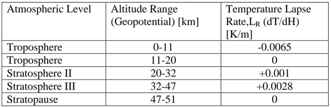
The temperature, pressure and density along with the altitude. The modeling of the three main characteristic of air is as follows. The pressure variation modeling in ISA is calculated using the hydrostatic equations, perfect gas law and the temperature lapse rate (LR) equations. LR is defined as rate of atmospheric temperature increase

with increasing altitude.

Table 2.2: Variation of TLR according to altitude

Atmospheric Level Altitude Range (Geopotential) [km] Temperature Lapse Rate,LR (dT/dH) [K/m] Troposphere 0-11 -0.0065 Troposphere 11-20 0 Stratosphere II 20-32 +0.001 Stratosphere III 32-47 +0.0028 Stratopause 47-51 0

The derivation of ISA can be found from [Cavcar, 2000, Daidzic, 2015, Anderson, 2005]. The change in temperature, pressure and density with altitude within the troposphere are given by the following equations:

(46)

0 {[g /(L R_R )] 1} a o o T T            (2.26) 1 R( 1) T  T L h h (2.27)

Figure 2.8: International Standard Atmosphere Figure 2.9: International Standard Atmosphere

This standard atmosphere is a generalization of the standard atmosphere. The lapse rate is assumed constant for each layer however some variation along the altitude may exist and also the gravitational force is not constant. However, this model is fairly accurate up to about 11km and most flight operation is limited to the troposphere and the stratosphere.

2.7 Flight dynamic equations

The many assumptions done in general for establishing the flight dynamics equations in view of the control of the flight of an aircraft and more specifically in view of the control of its trajectory using the control techniques are [Etkin and Reid, 1996] :

 The aircraft is assumed to be a rigid body

 The mass of the aircraft is taken as constant during a short period of time.

 The atmospheric parameters (static temperature and pressure, viscosity, volumic mass) are supposed to follow the standard atmospheric model.

(47)

 The modulus of the gravity vector is taken as constant in its direction towards the local vertical line.

A detailed computation of flight dynamics equations can be obtained from [Etkin and Reid, 1996],[Nelson, 1998],[Cook, 2013] and [Stevens and Lewis, 2003]. The rigid body assumption leads to consider the Euler equations relating the rotational speed components in the body frame to the rate of change of the attitude angles

( , , ) '  

  given in equation 2.28.

( )_bE

    (2.28)

1 sin tan cos tan

( ) 0 cos sin cos 0 tan cos                  _  _       (2.29)

The flight dynamic equations are governed by the force and moment equations according to Newton’s law:

Force equations: F mV_Bm_bEV_B (2.30) Moment equations: M I_bE_bEI_bE (2.31)

where the moments of inertia of the aircraft I is such as: 0 0 0 0 x xz y xz z I I I I I I             (2.32)

m is the aircraft mass and I is the aircraft inertial matrix in which the aircraft is assumed to be symmetrical (ie. Ixy=Iyx and Iyz=Izy are zero). VB=(u,v,w)’ is the

velocity of the center of gravity of the aircraft expressed in Body Frame. , bE =

(p,q,r)’ is the angular rotation vector of the body about the center of mass of the aircraft.

(48)

2.7.1 Forces

2.7.1.1 Gravity and Engine Thrust

As said before, the aircraft forces are made up by weight, thrust and also the aerodynamic forces. The Gravitational force, mg is directed normal from the earth surface, and is considered constant over the altitude envelope.

sin sin cos cos cos G F mg            _ _     (2.33)

As for the engine thrust, T, it is parallel to the aircraft body x-axis and the engine is mounted such that the thrust lies on the body-axes XZ-plane, offset from the center of gravity by ZTP along the z-axis. These gives:

0 0 T T F            (2.34)

2.7.1.2 The Aerodynamic forces

Figure 2.10: Aerodynamic Forces

The aerodynamic forces depend on other variables, like the angular rates (p, q, r) and

  Va Xa Za Ya L D Y

(49)

of control surfaces (a,e,r) and thrust command (Th) also influence these

aerodynamic forces.

From figure 2.10, it can be seen that the aerodynamic components, Lift (L), Drag (D) and Side Force (YF) are resolved in the aerodynamic frames (Xa,Ya,Za). The

components of the aerodynamic forces can be defined through the transformation matrix RWB such as:

X Y WB F Z F D F R Y F L       _         _      (2.35)

Where D is the drag force, YF is the lateral aerodynamic force and L is the lift force.

These aerodynamic forces are related to the dynamic pressure, the airspeed and the aircraft wing surface area through the following equation:

2 1 ( , , ) 2 a a D D  x y z V SC (2.36) 2 1 ( , , ) 2 a a L L  x y z V SC (2.37) 2 1 ( , , ) 2 F a a Y Y   x y z V SC (2.38)

where CD, CY and CL are respectively the dimensionless aerodynamic coefficients of

the drag, the side force and the lift which depend mainly on the angle of attack α and the side-slip angle β, and through the Mach number, on the airspeed and the flight level. The accepted expression of the aerodynamic forces coefficients are [Duke et al., 1988],[Etkin and Reid, 1996]:

(50)

0 E L L L Lq L e a q C C C C C V        (2.39) 0 2 2 r Y Y Y Yr Yp Y r a a rb pb C C C C C C V V         (2.40) 0 2 2 D D D D C C C C       (2.41)

From equation 2.30, the force equations in the body-axis reference frame can be written as: 1 sin ( x T) u rv qw g F F m       (2.42) 1 cos sin ( y) v pw ru g F m       (2.43) 1 cos cos ( _z) w qu pv g F m       (2.44)

2.7.2 Moments

As for the moments, the moment due to the thrust that lies on the body-axes XZ-plane, offsets from the center of gravity by ZTP along the z-axis as given by:

0 0 E TP M T Z     _  _     (2.45)

The aerodynamic moment MA=(LM,M,N) is expressed directly in the aircraft

Body-Axis Frame. The aerodynamic moments are also dependent on multiple variables as states for the aerodynamic forces. The moment of the aircraft is dependent on the airspeed, the dynamic pressure and also the aircraft reference chord length,c , and reference span, b. The accepted expressions of the aerodynamic moments are given by [Duke et al., 1988],[Etkin and Reid, 1996]:

2 1 ( , , ) 2 M M a a L L   x y z V S b C  (2.46)

(51)

2 1 ( , , ) 2 a a M M   x y z V S c C  (2.47) 2 1 ( , , ) 2 a a N N   x y z V S b C  (2.48)

And the contributing factor to the yawing moment CLM, pitching moment CM and

rolling moment CN coefficients are:

2 2 M a r L lo l lr lp l a l r a a rb pb C C C C C C C V V          (2.49) 2 2 e th M mo m m mq m e m th a a c qc C C C C C C C V V               (2.50) 2 2 a r N no n nr np n a n r a a rb pb C C C C C C C V V           (2.51)

From equations 2.30 and 2.31 moment equations in the body-axes reference frame can be written as:



2



2 1 { [( _y _z) _z _xz ] [( _x _y _z) _xz] } _z _xz x z xz p r I I I I I I I I p q I L I N I I I          (2.52)



2 2



1 ( z x) xz( ) T TP y q pr I I I p r M F Z I        (2.53)



2



2 1 { [( _x _y) _x _xz ] [( _x _y _z) _xz] } _z _xz x z xz r p I I I I I I I I r q I N I L I I I          (2.54)

2.8 A State Representation of Flight Dynamics

All these equation can be rewritten as a 12th order state representation considering the state variables p,q,r,,,,u,v,w,x,y and z. These equations are composed of:

(52)



2



2 1 { [( _y _z) _z _xz ] [( _x _y _z) _xz] } _z _xz x z xz p r I I I I I I I I p q I L I N I I I          (2.55a)



2 2



1 ( z x) xz( ) T TP y q pr I I I p r M F Z I        (2.56b)



2



2 1 { [( _x _y) _x _xz ] [( _x _y _z) _xz] } _z _xz x z xz r p I I I I I I I I r q I N I L I I I          (2.57c)

b) The aircraft Euler equations:

tan ( sin cos )

p q r      (2.58a) cos sin q r     (2.59b) sin cos cos q  r      (2.60c)

c) The acceleration components of the center of gravity in the body frame:

1 sin ( _x _T) u rv qw g F F m       (2.61a) 1 cos sin ( _y) v pw ru g F m       (2.62b) 1 cos cos ( _z) w qu pv g F m       (2.63c)

d) The speed components of the center of gravity of the aircraft in the LEF frame: ( ) ( ) ( ) ( ) ( ) ( ) ( ) ( ) ( ) ( ) ( ) ( ) ( ) ( ) ( ) ( ) ( ) ( ) ( ) ( ) ( ) ( ) ( ) ( ) ( ) ( ) ( ) ( ) ( ) x y z x c c s s c c s c s c s s u W y c s s s s c c c s s s c v W z s c s c c w W                                               _ _ _ _ _ _ _ _ _ _   _           _ _ _ _ _           (2.64)

The input parameters are composed of controlled parameters:

1. The total thrust of the engines (all engines are targeted to work identically) 2. The deflection of the main aerodynamic surfaces actuators (e.i. aileron,

(53)

3. The deflection of the secondary aerodynamic surfaces actuators (e.i. flaps, slats, spoiler, speed break) define the aerodynamic configuration of the aircraft on the medium term.

The uncontrolled parameters composed mainly of the wind components (Wx,Wy,Wz)

which can change with the atmosphere.

2.9 Global view of Flight Equations

As can be seen from the previous sections, the flight equations appear as a very complex system. However this complex system can be analyzed through the decoupling between the longitudinal and lateral motion and from the causal relationship between fast and slow dynamic modes. A subset of the aircraft flight dynamics system state’s variables are predominantly characterized by “fast dynamics” that is short time constants, high natural frequencies and bandwidth, and the “slow dynamics” with slow natural modes and longer transient response.

Figure 2.11: Global view of flight equations [Mora-Camino, 2014]

As shown in Figure 2.11, typically the piloting dynamics are faster than the guidance dynamics and they are the input to the guidance dynamics. In this thesis, the guidance dynamics will be addressed in order to design controllers to track specific aircraft reference trajectories. While it is assumed that the piloting dynamics are properly controlled by the autopilot.

The guidance dynamics are then given by:

a) The acceleration components of the center of gravity in the body frame: Attitude dynamics (fast) Guidance dynamics (slow) r q p



z

y

x

T   , , Engine dynamics T  , 

(54)

1 sin ( ) 1 cos sin ( ) 1 cos cos ( ) x T y z rv qw g F F m u v pw ru g F m w qu pv g F m       _ _ _ _          _ _ _ _             _ _ _      (2.65a)

b) The speed components of the center of gravity of the aircraft in the LEF frame: ( ) ( ) ( ) ( ) ( ) ( ) ( ) ( ) ( ) ( ) ( ) ( ) ( ) ( ) ( ) ( ) ( ) ( ) ( ) ( ) ( ) ( ) ( ) ( ) ( ) ( ) ( ) ( ) ( ) x y z x c c s s c c s c s c s s u W y c s s s s c c c s s s c v W z s c s c c w W                                               _ _ _ _ _ _ _ _ _ _   _           _ _ _ _ _           (2.65b) Equation 2.65 is composed of nonlinear ordinary differential equations and they are complex. Each equation consists of coupled state vectors. For simple analysis such as flight trimming and analysis of flight response on the longitudinal and lateral motions, these equations can be decoupled but this will not be discussed in this thesis. It can be found by further reading on the literature from [Nelson, 1998] and [Blakelock, 1991]. This thesis is only concern with the nonlinear ordinary differential equations.

2.10 Conclusion

From the above analysis, it appears that the guidance dynamics can be summarized by equations 2.65a and 2.65b. Once an autopilot system is available to control the attitude dynamics of the aircraft with short response time with respect to the guidance dynamics, the effective controller inputs of the guidance dynamics become the reference values for the pitch and bank angles and the total thrust of the engines, while the wind has indirect (equation 2.65a) and direct (equation 2.65b) effects. From the control point of view, the guidance dynamics form a strongly coupled nonlinear system where aircraft parameters (mass, configuration) have important influence.

(55)

CHAPTER 3

(56)

(57)

Chapter 3: Modern Flight Guidance Systems

3.1 Introduction

In this chapter a description and analysis of flight guidance systems on board modern air transport aircraft is performed. In the text, the terminologies are taken from Airbus aircraft but an equivalent Boeing aircraft also existed. The flight guidance function on board modern aircraft is designed to drive the aircraft along a safe and efficient trajectory. This function is embedded in the Flight Management System (FMS) and operates in close relation with the Navigation functions. Flight plans are generated by the Flight Management System (FMS) in accordance with tactical choices of the airline operating that aircraft. In general, a flight plan combines lateral and vertical parts composed of different segments. Each segment corresponds in general to some local objective with respect to the guidance variables. This induces a sequence of different guidance modes along the flight from initial climb to landing. A flight plan can be followed automatically by the flight guidance system where the FMS provides the successive decisions with respect to the shift from one guidance mode to the next and to the choice of the guidance target parameters. In that case, the guidance system is managed by the FMS. In other situations, the pilot takes over the control of the flight guidance systems, imposing a different sequence of modes (selected mode) and guidance parameters. This second situation happens normally at take-off and when the ATC produces injunctions with respect to the trajectory of the aircraft. This can also happen when the pilot reacts to a guidance alarm, including or not a resolution advice.

Pilot

Flight Plans generation

MCDU Automatic Automatic Piloting Rotational Dynamics FCU Guidance Dynamics MANAGED

SELECTED _{Mechanical Backup}

Navigation

(58)

Figure 3.1: Overall classical structure of flight control systems [Mora-Camino, 2014]

So in this chapter, to understand better the organization and operation of the flight guidance systems, first, a description of up-to-date FMSs and the main characteristics of the generated flight plans which must be achievable by the flight guidance system will be introduced.

3.2 The Flight Management Systems

3.2.1 Flight Management Functions

Today the Flight Management System integrates closely related functions to allow the aircraft and its pilot to perform a safe and efficient flight. These related functions are:

- The navigation function which allows to appreciate any difference between the current position of the aircraft and its planned one, possibly for correction through the guidance function.

- The trajectory predictive function which provides information and predictions about the actual flight, allowing for instance to check if delays resulting from late departure or different winds than forecasted can be compensated.

- The flight planning function which helps the pilot to choose the horizontal track to be followed all along the flight.

- The performance function which computes for a particular flight characteristic parameters such as take-off speed and an optimized vertical profile to be fed to the guidance system.

- and finally the flight guidance function.

It appears rather difficult to distinguish the flight guidance system from the other systems imbedded in the flight management system, especially when, as is generally the case with modern aircraft where all these functions are developed

Flight guidance along 3D+T trajectories and space indexed traffic management

T

T

H

H

È

È

S

S

E

E

DOCTORAT DE L’UNIVERSITÉ DE TOULOUSE

M

AB WAHID

ACKNOWLEDGMENT

ABSTRACT

RESUME

CONTENTS

LIST OF FIGURES

LIST OF TABLES

NOMENCLATURE

CHAPTER 1

Chapter 1: General Introduction

CHAPTER 2

TRANSPORTATION AIRCRAFT FLIGHT

DYNAMICS

Chapter 2: Transport Aircraft Flight Dynamics

2.1 Introduction

2.2 The reference frames

2.3 Frame Transformations

2.4 Aircraft Speeds and Wind Speed

     

     













2.5 Flight path angle

2.6 The Standard Atmosphere

2.7 Flight dynamic equations

2.7.1 Forces

2.7.2 Moments













2.8 A State Representation of Flight Dynamics













2.9 Global view of Flight Equations







z

y

x

2.10 Conclusion

CHAPTER 3

Chapter 3: Modern Flight Guidance Systems

3.1 Introduction

3.2 The Flight Management Systems

3.2.1 Flight Management Functions