HAL Id: inserm-00335194
https://www.hal.inserm.fr/inserm-00335194
Submitted on 28 Oct 2008
HAL is a multi-disciplinary open access
archive for the deposit and dissemination of
sci-entific research documents, whether they are
pub-lished or not. The documents may come from
teaching and research institutions in France or
abroad, or from public or private research centers.
L’archive ouverte pluridisciplinaire HAL, est
destinée au dépôt et à la diffusion de documents
scientifiques de niveau recherche, publiés ou non,
émanant des établissements d’enseignement et de
recherche français ou étrangers, des laboratoires
publics ou privés.
The Labeling of Cortical Sulci using Multidimensional
Scaling
Mani Meena, Srivastava Anuj, Barillot Christian
To cite this version:
Mani Meena, Srivastava Anuj, Barillot Christian. The Labeling of Cortical Sulci using
Multidimen-sional Scaling. MICCAI Workshop - Manifolds in Medical Imaging: Metrics, Learning and Beyond,
Sep 2008, New-York, United States. �inserm-00335194�
The Labeling of Cortical Sulci using
Multidimensional Scaling
Meena Mani1, Anuj Srivastava2, and Christian Barillot1
1 INRIA/INSERM, Visages Project, IRISA, Rennes, France. 2 Department of Statistics, Florida State University, Tallahassee, USA.
{memani, cbarillot}@irisa.fr, [email protected]
Abstract. The task of classifying or labeling cortical sulci is made diffi-cult by the fact that individual sulci may not have unique distinguishing features and usually need to be identified by a multivariate feature set that takes the relative spatial arrangement into account. In this paper, classical multidimensional scaling (MDS), which gives a geometric inter-pretation to input dissimilarity data, is used to classify 180 sulci drawn from the ten major classes of sulci. Using a leave-one-out validation strat-egy, we acheive a success rate of 100% in the best case and 78% in the worst case. For these more difficult cases, we propose a second stage of classification using shape based features. One of these features is the geodesic distance between sulcal curves obtained from a new open curve representation in a geometric framework.
With MDS, we offer a simple and intuitive approach to a challenging problem. Not only can we easily separate left and right brain sulci, but we also narrow the classification problem from, in this case, a 10-class to a 2-class problem. More generally, we can identify a region-of-interst (ROI) within which one can carry out further classification.
1
Introduction
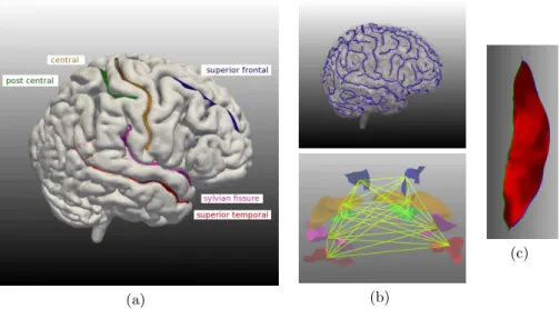
The large variability present in the human brain cortex makes it one of the most challenging of brain anatomies to segment, label, classify or model. The sulci, which are fissures or grooves in the cortical surface (Figure 1), vary not just in their shape and placement, but even in their number. Even so, the underlying architectonic and functional organization of the brain influences to some degree the size, shape and placement of the folding patterns [1]. The length, depth, the pure shape (i.e. after removing scaling, rotation and translation), the spatial arrangement and orientation of some of these individual sulci are characteristic features shared across a population. Collectively, these features can form the basis for classification, labeling and the study of selective differentiation of tissue that results from neurodegenrative pathologies, the action of genes or even as a result of cognitive activity. This study fills an important need and can lead to such wide-ranging applications as landmark or guidance-based neurosurgical procedures or the differential diagnosis of degenerative brain disease.
Accurate sulcal identification can be a challenge even for expert neuroanatomists. A strategy that is used in manual annotation is to identify sulci in relation to
the major sulci for which we can show consistent anatomical correspondence be-tween subjects. The major sulci provide a context and coupling this information with shape attributes, which are usually not unique to a class of sulci, helps in identification [2]. The automated and semi-automated labeling methods that incorporate this idea typically involve using a large feature set and computa-tionally intensive algorithms [3]. We propose a simpler approach, not considered before, which uses only distance or dissimilarity data to individually identify unlabeled sulci against a reference graph (Figure 1(b)).
Multidimensional scaling (MDS) is a technique that gives a geometric inter-pretation to dissimilarity data and is a natural tool for such an application. By minimizing a loss function calculated for different possible configurations, we can assign a set of coordinates to objects. The resulting map, or embedding, places objects that have similar attributes close to each other. MDS can be used as a classification tool by introducing unlabeled sulci to an existing map. Membership is then assigned to the nearest node using a minimum distance classifier.
There is a growing recognition, in medical image analysis, that to take advan-tage of the full range of information presented in an image, one has to consider shape attributes. Sulcal shape analysis has typically used a multivariate fea-ture set to describe shape attributes such as angle, curvafea-ture, depth, length [4]. To date, little work has been done using a formal definition of shape spaces of sulcal curves. In this paper, we use a new geometric representation for studying shapes of three-dimensional sulcal curves using metrics invariant to the standard shape-preserving transformation.
In Section 2 we briefly explain the MDS method and how it is used for labeling the major sulci. Next, we present a new shape representation for open curves in Section 3. Though the formalism itself has a wider scope, the focus in this paper is its application to sulcal curves. In Section 4, we describe the other features used in our dissimilarity calculations. Finally, in Section 5, we present the preliminary results. In the discussion that follows, Section 6, we outline our plans to develop this classification method further.
2
Metric Multidimensional Scaling
Multidimensional scaling is a method that allows us to compute an optimal configuration, X, for a set of n observations using only their interpoint distances. If ∆ = [δij] is a non-negative, symmetric matrix of dissimilarities computed from a set of (hidden) coordinates, Xrof rank r, with MDS, we can represent Xr as Xd, d ≤ r, such that the distance matrix D computed from it is close to ∆. An intermediate step would be to derive the scalar product matrix, B = XXT, from the squared dissimilarities by double centering. An eigen decomposition, B = Γ ΛΓT, gives us Λ, a diagonal matrix of eigenvalues, and Γ, a matrix of orthonormal eigenvectors. X, the square root of XXT, is then Γ Λ1
2. Since B is of
(a) (b)
(c)
Fig. 1.(a) The five major sulci used in this study. (b) Top: Sulcal curves, in blue, form a complex and widely varying pattern on the cortex. Bottom: Graph representation where the distances are the edges and the sulci are the nodes. (c) An individual sulcus. The top or superficial curve, which points in the direction of the outer cortex, is in blue. The bottom curve is in green.
the stress function:
σ(x1, . . . , xn) = n X i=2 i−1 X j=1 (kxi− xjk − δij)2. (1) 2.1 Out-of-sample Embedding
For classification, our objective is to introduce k additional points, y1,. . . ,yk, without disturbing an existing representation. Using Eqn. 1 to embed n + k points, however, gives an entirely new map. Intead, if we optimize
σ(y1, . . . , yk) = 2 n X i=1 k X j=1
(kxi− yjk − ai(n+j))2+ k X i=1 k X j=1
(kyi− yjk − a(n+i)(n+j))2,
where A = [aij] is the augmented (n + k) × (n + k) dissimilarity matrix, we can get yi, the coordinates for the k points, while xi, the original points remain fixed. This treatment, detailed in Trosset et al. [5], is an extension of the optimization solved by Eqn. 1.
3
Elastic Shape Analysis of Sulcal Curves
We use a new square-root velocity description for shapes of three-dimensional sulcal curves. This representation is related to the velocity function used in [6]
and to the complex square-root representation for planar curves in [7]. The advantage of this representation, first proposed by Joshi et al. [8] for closed curves, is that the resulting pre-shape becomes a unit hypersphere space and one can use the geometry of the sphere for computations.
3.1 Curve Representation and Pre-Shape Space
Let β : [0, 1] → R3 be a unit-length, parameterized curve such that its speed k ˙β(t)k is non-zero everywhere. We define its square-root velocity function as:
q(t) = qβ(t)˙ k ˙β(t)k
, t ∈ [0, 1] .
The space of all square-root velocity representations of curves in R3, B, is a unit hypersphere and submanifold of L2([0, 1], R3). Since B is a Riemannian manifold with the inner product metric hw1, w2i , we can derive an exponential and an inverse exponential map. We can also compute geodesic paths between curves using
ψ(t) = 1
sin(θ)[sin(θ − t)q1+ sin(t)q2] , (2) where θ = cos−1(hq1, q2i) is the geodesic distance, denoted by dc(q1, q2), between two points.
3.2 Shape Space
The elements of B do not represent the shape of a curve uniquely. Any re-parametrization or rigid rotation of β, results in a different square-root velocity function, q, while preserving its shape. We will call B the pre-shape space of open curves. This variability can be represented using the actions of the re-parameterization group, Γ , and the rotation group, SO(3), on B. These actions commute and both groups act on B in an isometry. We can thus define the shape space as:
S = B/(Γ × SO(3).
Let [q] denote an orbit resulting from all possible re-parameterizations and rota-tions of a curve denoted by q ∈ B. S is the set of all such orbits and it inherits a Riemannian structure from B, under which, the geodesic distance between two orbits [q1] and [q2] is:
ds([q1], [q2]) = min
γ∈Γ,O∈SO(3)dc(q1,p ˙γOq2(γ)) . (3) The geodesic is given by [ψt], where ψt is the geodesic in B between q1 and p ˙γ∗O∗q2(γ∗). Here (O∗, γ∗) are the optimal transformations of q2that minimize dc. A closer look at that distance function reveals:
argmin γ∈Γ,O∈SO(3)
cos−1Dq1,p ˙γOq2(γ)E= argmin γ∈Γ,O∈SO(3)
This equality says that to minimize the arc length on a unit sphere is the same as minimizing the chord length.
3.3 Karcher Means of Open Curves
To get the mean shape for a given set of curves, we compute a Karcher mean,
¯ µn= argmin [q]∈S n X i=1 ds([q], [qi])2 . (5)
A gradient-based approach to find the minimum is commonly used for finding means on nonlinear manifolds. The extrinsic mean, µ 7→ µ/kµk, is used to ini-tialize the gradient search. We update µ by computing the exponential map, expµ(ǫ¯v), to get a local minimizer for the cost function in Eqn. 5.
4
Feature Set
For the MDS evaluation, we used four descriptors, position, depth, length and orientation, in addition to shape. These contain physical information not cap-tured in the shape of a 1D curve alone. For each of these descriptors, our features were the distances between sulci or the class averages of sulci.
Spatial PositionThe mid-point of each sulcal curve was used for the position coordinates.
Mean DepthThe depth profile for each sulcus was first obtained by resampling 100 points along the length of the sulcus and computing the distance between points on the top sulcal curve with corresponding points on the bottom curve. The mean depth was then calculated by averaging these.
LengthThe length of a sulcus was computed using R1
0 k ˙β(t)kdt, the length of the curve β.
Orientation Using singular value decomposition (SVD), the relative orienta-tions, O, between sulcal curves were computed for each subject.
The class average for each of these descriptors was calculated by averaging across the 18 subjects. For the relative orientation, the average was obtained by computing a SVD ofP
iOi. The Karcher mean gave us the mean shape. The distance matrix was computed using the feature distances between two sulci. For position we computed a euclidean distance. For depth and length, we used an absolute distance. For orientation, we used do=k log(O√1OT2)k
2 , where k.k is the Frobenius norm. For shapes, the geodesic distance was used.
The composite distance between any two sulci was also computed by using a combination of the scaled distances, d = w1ds+ w2dp+ w3dd + w4dl+ w5do, where the wi could be chosen by trial and error.
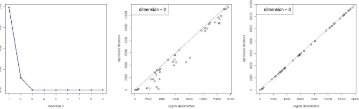
Fig. 2.Evaluating the number of dimensions required to represent the data. The scree plot (left), shows that 3 dimensions is adequate for the MDS map. The Shepard plot for 2D data (middle) shows more spread than the corresponding 3D plot (right).
5
Results
5.1 Data and Initial Processing
We used a database of 18 T1-MR 3D SPGR brain images of healthy subjects, matched for sex (male), handedness (right), and age (35 ± 10 years). Five major sulci, the central, postcentral, superior frontal, sylvian fissure and superior tem-poral, were extracted from each hemisphere using the method described in [2, 9]. This gave us 18 × 10 = 180 sulci for classification. These primary sulci were chosen because they can consistently be identified in all normal individuals. The left and right precentral sulci were later included to test and extend the classi-fier. This expanded the dataset to 18 × 12 = 216 sulci. For analysis, the top and bottom sulcal lines extracted from each sulcus (see Figure 1(c)), were used.
5.2 Evaluating Dimensionality, Assessing Fit
MDS reproduces a high dimensional input in a lower dimensional space. A scree test was used to determine the dimension that best represents the sulcal data. In Figure 2, an elbow in the plot at d = 3, represents the optimal dimension beyond which only minor reductions in stress are acheived. The Shepard diagram, which plots the scaled MDS distances against the original dissimilarity data, was then used to assess fit for 2 and 3D data. A good fit is indicated by a minimal spread in the scatter plot and evidence of a monotonically ascending relation. A comparison between the two Shepard plots, shows that the output distances are highly correlated to the input dissimilarities for the 3D data. As a final test, the MDS map we obtain, reflects the actual arrangement of sulci in the brain.
5.3 Classification
Our goal was to label segmented sulci making no assumptions about pre-defined relationships or any other information. For this we designed a 10-class MDS classifier. We evaluated the classification using leave-one-out (LOO) cross-validation. The 18 sulci for each of the 10 sulcal classes were split 17:1 into a training set and a testing set. As expected, the best results for the 18 LOO it-erations were obtained when spatial distances were used for the dissimilarities. We got an overall true positive rate of 90% and 90.6% for the top and bottom sulcal classifiers respectively (Table 1), and were able to correctly label all the superior frontal sulci (100%). The sylvian fissure, the most difficult class, had a success rate of 78%. The sylvian fissure is composed of a number of small folds that are difficult to extract completely. As a result, the features used to describe the sylvian fissure have a noisy multimodal distribution.
Classification was also done for shape, using geodesic paths for distances, and for scaled combinations of shape, position, length and depth. The shape classi-fier labeled all the central sulci, which are very regular, but was less successful with the other classes. Combining the features did not improve the success rate. Rather, the results achieved by the spatial distance classifier were compromised (Figure 4). The depth and length classifiers could not discriminate right and left brain sulci, and while the orientation information improved results in cases where the orientations of the sulci differed, these were offset by the errors introduced.
6
Discussion
Fig. 3.Depth boxplot. An MDS spatial distance classifier offers several
ad-vantages. First, if n is the number of classes, we need only make n(n−1)2 distance measurements, off-line, to construct a reference map. For classification, data from unlabeled sulci supplement this distance ma-trix. Second, our results suggest that we can very quickly assign a given sulcus to a small region of the left or right hemisphere. All 180 sulci were correctly identified when we relaxed the classification criteria to include the second nearest sulcus. Third, the clas-sifier is robust to normal population variation. The results we obtained, were for data that had not been spatially normalized. Both the top and more stable bottom sulcal classifiers, moreover, gave comparable results (Table 1). We were even able to correctly iden-tify a displaced and distended superior frontal sulcus, taken from a tumor patient.
Central to our approach to sulcal classification is the use of a reference graph. This imposes several constraints which narrow down possible solutions so that a high average classification rate is achieved. The classifier works best when only
a small number of well separated sulcal classes are used in the training set. We saw the performance degrade from 90.6% to 84.3% when two additional classes, the left and right precentral sulcus were added (Figure 5). Based on preliminary results and characterization, we propose a two stage classification scheme where the spatial distance classifier will serve as a front end to identify a region of interest. Specialized feature classifiers can then be applied in the second stage. A depth classifier, for instance, can discriminate between the sylvian fissure(SF) and the superior temporal sulcus(ST) (Figure 3). These two sulci were sometimes misclassified, one for the other, with the position classifier.
References
1. Van Essen, D.: A tension-based theory of morphogenesis and compact wiring in the central nervous system. Nature 385(6614) (1997) 313–318.
2. Le Goualher, G., Procyk, E., Collins, D.L., Venugopal, R., Barillot, C., Evans, A.C.: Automated extraction and variability analysis of sulcal neuroanatomy. IEEE Trans. Med. Imaging 18(3) (1999) 206–217.
3. Rivi`ere, D., Mangin, J.F., Papadopoulos-Orfanos, D., Martinez, J.M., Frouin, V., R´egis, J.: Automatic recognition of cortical sulci using a congregation of neural networks. In: MICCAI ’00. (2000) 40–49.
4. Hurdal, M.K., Gutierrez, J.B., Laing, C., Smith, D.A.: Shape analysis for automated sulcal classification and parcellation of MRI data. J. Comb. Optim. 15(3) (2008) 257–275.
5. Trosset, M.W., Priebe, C.E.: The Out-of-Sample Problem for Classical Multidimen-sional Scaling. Computational Statistics & Data Analysis 52(10) (2008) 4635–4642. 6. Balov, N., Srivastava, A., Li, C., Ding, Z.: Shape analysis of open curves in R3 with applications to study of fiber tracts in DT-MRI data. In: EMMCVPR. (2007) 399–413.
7. Michor, P.W., Mumford, D., Shah, J., Younes, L.: A metric on shape space with explicit geodesics. Rend. Lincei Mat. Appl. 9 (2008) 25–57.
8. Joshi, S., Klassen, E., Srivastava, A., Jermyn, I.H.: A novel representation for Riemannian analysis of elastic curves in Rn. In: Proc. IEEE Computer Vision and Pattern Recognition (CVPR), Minneapolis, USA (June 2007)
9. Le Goualher, G., Barillot, C., Bizais, Y.: Modeling cortical sulci with active ribbons. IJPRAI 11(8) (1997) 1295–1315.
Acknowledgement
MM would like to thank Michael Trosset for making his R-code for out-of-sample embedding available.
Table 1.Confusion Matrix for MDS Spatial Distance LOOCV.
The true positive rate (blue), gives the % of the sulci correctly identified in 18 LOO tests. The off-diagonal terms (red) give the % of false negatives.
Top Sulcal Curve Bottom Sulcal Curve
True Label 1 2 3 4 5 6 7 8 9 10 1 2 3 4 5 6 7 8 9 10 T es t L a b el Left central 1 10016 8916 L. postcentral 2 84 1184 L. sup. frontal 3 100 100 L. sylvian fissure 4 8411 8411 L. sup. temporal 5 1689 1689 Right central 6 94.522 94.522 R. postcentral 7 5.5 78 5.5 78 R. sup. frontal 8 100 100 R. sylvian fissure 9 8916 94.5 5.5 R. sup. temporal 10 1184 5.5 94.5
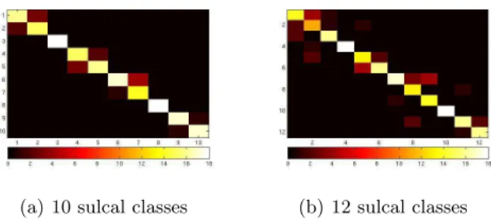
Fig. 4.Confusion map for MDS classification: the shape distance results (left) improve considerably when the shape & spatial distances (middle) are combined; the spatial distance alone (right) gives the best perfomance.
(a) 10 sulcal classes (b) 12 sulcal classes
Fig. 5.The results for the spatial distance deteriorated when the two precentral sulci were added, increasing the number of classes to 12. The precentral sulcus was sometimes miscategorized as the adjacent sylvian fissure, the central or superior frontal sulcus.