Learning and Using Structures for Constraint Acquisition

HAL Id: tel-01816945

https://tel.archives-ouvertes.fr/tel-01816945

Submitted on 15 Jun 2018

HAL is a multi-disciplinary open access

archive for the deposit and dissemination of

sci-entific research documents, whether they are

pub-lished or not. The documents may come from

teaching and research institutions in France or

abroad, or from public or private research centers.

L’archive ouverte pluridisciplinaire HAL, est

destinée au dépôt et à la diffusion de documents

scientifiques de niveau recherche, publiés ou non,

émanant des établissements d’enseignement et de

recherche français ou étrangers, des laboratoires

publics ou privés.

Learning and Using Structures for Constraint

Acquisition

Abderrazak Daoudi

To cite this version:

Abderrazak Daoudi. Learning and Using Structures for Constraint Acquisition. Other [cs.OH].

Uni-versité Montpellier; UniUni-versité Mohammed V (Rabat), 2016. English. �NNT : 2016MONTT316�.

�tel-01816945�

Université Mohammed V Faculté des Sciences de Rabat

Collège doctoral du languedoc-roussillon Université de Montpellier

N◦_{d’ordre: . . . .}

THÈSE DE DOCTORAT

présentée par

Abderrazak D

AOUDI

Discipline : Sciences de l’ingénieur

Spécialité : Informatique

L

EARNING AND

U

SING

S

TRUCTURES

FOR

C

ONSTRAINT

A

CQUISITION

Soutenue le 10 Mai 2016 devant le jury composé de :

M. Mohammed BENKHALIFA Professeur U. Mohammed V, Maroc Président

M. Christian BESSIERE DR CNRS U. de Montepellier, France Directeur de thèse M. El Houssine BOUYAKHF Professeur U. Mohammed V, Maroc Directeur de thèse M. Redouane EZZAHIR Professeur U. Ibn Zohr, Maroc Rapporteur

Mme Souhila KACI Professeur U. de Montepellier, France Examinateur Mme Élise VAREILLES HDR École des Mines d’Albi, France Rapporteur

i

To my parents

To my sisters and brothers

Contents

2.1.2 Examples of Constraint Networks . . . 14

2.1.3 Solving Methods . . . 16

2.2 Constraint Language and Basis . . . 17

2.3 Concept Learning . . . 18

2.4 Constraint Acquisition . . . 18

2.4.1 Passive Learning . . . 19

2.4.2 Active Learning . . . 20

2.4.3 Constraint Acquisition as a Search . . . 20

2.5 Existing Constraint Acquisition Systems. . . 20

2.5.1 CONACQ.1. . . 21

2.5.2 CONACQ.2. . . 23

2.5.3 MODELSEEKER. . . 24

3 Constraint Acquisition with Generalization Queries 31

3.1 Introduction . . . 31

3.2 GENACQAlgorithm . . . 33

3.2.1 Description of GENACQ . . . 34

3.2.2 Completeness and Complexity . . . 34

3.2.3 Illustrative Example . . . 35

3.2.4 Using Generalization in QUACQ . . . 36

3.3 Strategies . . . 37

3.3.1 Query Selection Heuristics . . . 38

3.3.2 Using Cutoffs. . . 39

3.4 Experimentations . . . 39

3.4.1 Benchmark Problems . . . 39

3.4.2 Results . . . 40

3.5 Conclusion . . . 44

4 Detecting Types of Variables for Constraint Generalization 45 4.1 Introduction . . . 45

4.2 MINE&ASKAlgorithm . . . 48

4.2.1 Description of MINE&ASK . . . 48

4.2.2 M-QUACQ Algorithm . . . 50

4.3 An Illustrative Example . . . 50

4.4 Extraction of Potential Types . . . 51

4.4.1 Optimizing Modularity . . . 51

4.4.2 Edge Betweenness Centrality . . . 53

4.4.3 Quasi-cliques Detection . . . 53

4.5 Experimentations . . . 54

4.5.1 Benchmark Problems . . . 55

4.5.2 Results . . . 56

4.6 Conclusion . . . 57

5 Constraint Acquisition with Recommendation Queries 59 5.1 Introduction . . . 59

5.2 PREDICT&ASK Algorithm. . . 60

5.2.1 Description of PREDICT&ASK . . . 61

5.2.2 Using Recommendation in QUACQ . . . 62

5.2.3 Complexity Analysis . . . 62

5.3 An Illustrative Example . . . 63

5.4 Prediction Strategies . . . 65

5.4.1 Adamic-Adar Index (AA) . . . 65

5.4.2 Leicht-Holme-Newman Index (LHN). . . 66

5.5 Experimental Evaluation. . . 66

5.5.1 Benchmark Problems . . . 66

5.5.2 Results . . . 67

CONTENTS v 5.7 Conclusion . . . 71

6 Conclusion & Perspectives 73

Bibliography 75

List of Figures 83

Acknowledgments

The research work presented in this thesis has been conducted in the Laboratory of Informatics Applied Mathematics, Artificial Intelligence and Pattern Recognition (LIMIARF), Faculty of Sciences, University Mohammed V of Rabat, Morocco, and the Laboratory of Informatics, Robotics and Microelectronics of Montpellier (LIRMM), University of Montpellier, France.

This thesis has been done in collaboration between University Mohammed V of Rabat, Morocco, and University of Montpellier, France, under the financial support of the scholarship Averroès funded by the European Commission.

Firstly, I would like to express my deepest gratitude to my supervisors Professor El Houssine Bouyakhf and Professor Christian Bessiere. I will always be grateful for all the support, guidance, encouragement they have given me during these three years. It was a real pleasure for me to work with them. They are so highly moti-vated, enthusiastic and passionate about science. Their guidance, suggestions and relevant feedback helped me a lot to progress and to continue my research in the right direction.

I would like to express my sincere gratitude to the jury for the interest according to my work. I gratefully acknowledge Mr. Mohammed Benkhalifa, Professor at Faculty of sciences, University Mohammed V of Rabat, Morocco, for accepting to chair the jury of my dissertation. I would like to thank Ms. Souhila Kaci, Professor at University of Montpellier, France, for accepting to exanimate my thesis. I am most grateful to my reviewers Ms. Elise Vareilles, Associate Professor (HDR) at Ecole des Mines d’Albi, France, and Mr. Redouane Ezzahir, Associate Professor (PH) at University of Ibn Zohr, Morocco. I thank them all for their comments and fruitful discussions.

The published research works of this thesis have been done in collaboration with so highly motivated, smart and enthusiastic coauthors. I want to thank them for

their hard work and teamwork. I cannot thank my coauthors without giving my special gratitude to Younes Mechqrane, Nadjib Lazaar and Remi Coletta.

My thanks go also to the staffs of the LIRMM and LIMIARF Laboratories. I would like to thank all past and present colleagues at the LIRMM and LIMIARF for the joyful and pleasant working environment. I especially acknowledge the members of the Coconut team: Gilles, Joel, Phillipe, Natasa, Gaelle, Olivier, Nicolas, Mehdi and Robin, and the members of IA team of LIMIARF: Imade, Saida, Yousra, Amine, Mehdi, Zakarya and Ghizlan.

During this thesis, I have been blessed with a cheerful group of friends. I would like to particularly thank Amine, Nawfal, Adil, Mohamed, Abdelhak, Youssef K., Youssef M., Mouad, Lhassan, Salim, Jaouad, Younes and Ahmed.

Last but not the least; I would like to thank my family: my parents, my sisters and brothers for their unconditional support, encouragement and endless love.

Dr. Abderrazak Daoudi Montpellier, May 23, 2016

Abstract

Constraint Programming is a general framework used to model and to solve complex combinatorial problems. However, modeling a problem as a constraint network requires significant expertise in the field. Such level of expertise is a bottleneck to the broader up-take of the constraint technology. To alleviate this issue, several constraint acquisition systems have been proposed to assist the non-expert user in the modeling task. Neverthe-less, in these systems the user is only asked to answer very basic questions. The drawback is that when no background knowledge is provided, the user may need to answer a large number of such questions to learn all the constraints. In this thesis, we show that using the structure of the problem under consideration may improve the acquisition process a lot. To this aim, we propose several techniques. Firstly, we introduce the concept of gen-eralization query based on an aggregation of variables into types. Secondly, to deal with generalization queries, we propose a constraint generalization algorithm, named GENACQ,

together with several strategies. Thirdly, to make the build of generalization queries totally independent of the user, we propose the algorithm MINE&ASK, which is able to learn the structure, during the constraint acquisition process, and to use the learned structure to generate generalization queries. Fourthly, toward a generic concept of query, we introduce the recommendation query based on the link prediction on the current constraint graph. Fifthly, we propose a constraint recommender algorithm, called PREDICT&ASK, that asks recommendation queries, each time the structure of the current graph has been modified. Finally, we incorporate all these new generic techniques into QUACQalgorithm leading to

three boosted versions, G-QUACQ, M-QUACQ, and P-QUACQ. To evaluate all these tech-niques, we have made experiments on several benchmarks. The results show that the extended versions improve drastically the basic QUACQ.

Keywords: Artificial Intelligence (AI), Constraint Programming (CP), Constraint Satisfaction

Problems (CSP), Constraint Acquisition, Learning, Graph Community Detection, Recommenda-tion Systems.

Résumé

La Programmation par Contraintes est un cadre général utilisé pour modéliser et ré-soudre des problèmes combinatoires complexes. Cependant, la modélisation d’un problème sous forme d’un réseau de contraintes nécessite une bonne expertise dans le domaine. Ce niveau d’expertise est un obstacle majeur pour une large diffusion de la programmation par contraintes. Pour remédier à ce problème, plusieurs systèmes d’acquisition de contraintes ont été proposés pour aider l’utilisateur dans la tâche de modélisation. Dans ces systèmes, l’utilisateur ne répond qu’à des questions très simples. L’inconvénient est que lorsqu’aucune connaissance de base n’est fournie, l’utilisateur peut avoir besoin de répondre à un grand nombre de questions pour apprendre toutes les contraintes. Dans cette thèse, nous mon-trons que l’utilisation de la structure du problème peut améliorer considérablement le pro-cessus d’acquisition. Pour ce faire, nous proposons plusieurs techniques. Tout d’abord, nous introduisons le concept de requête de généralisation basée sur une agrégation de vari-ables sous forme de types. Deuxièmement, pour faire face aux requêtes de généralisation, nous proposons un algorithme de généralisation de contraintes, nommé GENACQ, ainsi que plusieurs stratégies. Troisièmement, pour rendre la construction de requêtes de généralisa-tion totalement indépendante de l’utilisateur, nous proposons l’algorithme MINE&ASK, qui

est en mesure d’apprendre la structure au cours du processus d’acquisition, et d’utiliser la structure apprise pour générer des requêtes de généralisation. Quatrièmement, pour aller vers un concept générique de requête, nous introduisons la requête de recommandation basée sur la prédiction de liens dans le graphe de contraintes apprises jusqu’à présent. Cinquièmement, nous proposons un algorithme de recommandation de contraintes, appelé PREDICT&ASK, qui demande à l’utilisateur de classifier des requêtes de recommandation chaque fois que la structure du graphe courant a été modifiée. Enfin, nous intégrons toutes ces nouvelles techniques dans l’algorithme QUACQ, menant à trois nouvelles versions, à savoir G-QUACQ, M-QUACQ, et P-QUACQ. Pour évaluer toutes ces techniques, nous avons fait des expérimentations sur plusieurs jeux de données. Les résultats montrent que les versions étendues améliorent considérablement le QUACQde base.

Mots clefs : Intelligence Artificielle, Programmation par contraintes, Problèmes de

satis-faction de contraintes, Acquisition de contraintes, Détection de communautés, Systèmes de recommandation.

C

1

Introduction

Constraint Programming (CP) is a very active research area within Artificial In-telligence (AI), and its importance has increased dramatically within the last years. CP is a highly successful technology for solving a wide range of combinatorial prob-lems, such as scheduling, resource allocation, and design. Nowadays, a number of companies, like ILOG and Dash Optimization, sell constraint programming toolkits, which are used by companies as diverse as Amazon.com, British Airways, Cisco, Ford, HP, SNCF, and Volvo.

Constraint programming is a declarative style of modeling combinatorial prob-lems. The user identifies the decision variables, their possible domain of values, and specifies constraints over the allowed values. For instance, the constraint X1+X2≤X3 specifies that any combination of values for variables X1, X2and X3 has to be such that the sum of X1and X2less than or equals X3. Sophisticated AI search techniques like constraint propagation, which allow to prune irrelevant parts of the search tree, and chronological backtracking can then be used to find solutions.

Unfortunately, modeling a combinatorial problem as a constraint network re-mains limited to specialists in the field. However, it is well known that modeling a combinatorial problem in the constraint formalism requires significant expertise in constraint programming [Freuder, 1999; Puget, 2004]. Such a level of knowl-edge prevents non-expert users from being able to use constraint networks without the help of an expert. Consequently, this has a negative effect on the uptake of constraint technology in the real-world by novices.

One answer to the task of modeling is constraint acquisition, which is an active research field that lies in the conjunction of two fields, namely Constraint Program-ming and Machine Learning. The idea behind constraint acquisition is to assist

a non-expert user in modeling her problem as a constraint network. Several con-straint acquisition systems have been introduced in the last decade [Bessiere et al., 2005, 2007; Lallouet et al., 2010; Beldiceanu and Simonis, 2012; Bessiere et al., 2013]. Unfortunately, Most of these constraint acquisition systems interact with the user by asking her to classify an example as positive or negative. Such queries do not use the structure of the problem and can thus lead the user to answer a large number of queries. Hence, it can be hard to put constraint acquisition in practice.

The propose of this thesis is to provide new approaches to constraint acquisition in order to make it more efficient in practice. However, we show that learning and using the structure of the problem under consideration may accelerate the process of learning a lot. To this end, we introduce two new concept of queries that use the structure of the problem. The first one, called generalization query, is an op-portunistic query based on the aggregation of variables into types. Generalization query asks the user whether or not a learned constraint can be generalized on other variables of the same types as those of the learned constraint. The second query, called recommendation query, based on the analysis of the partial constraint graph learned so far, by using techniques borrowed from data mining and link predic-tion in dynamic graphs. Recommendapredic-tion query asks the user whether or not a predicted constraint may belongs to the target network.

We propose several algorithms that manage these new concept of queries. First, we propose GENACQalgorithm, which is a generic algorithm that asks generalization queries. Second, we present MINE&ASK algorithm, which is able to learn types during the constraint acquisition process and to use the extracted types to build generalization queries. Third, we introduce PREDICT&ASK, which is a constraint recommender algorithm that uses the structure, of the constraint graph learned so far, to predict new constraints that may belong to the target network, and to ask the user to classify recommendation queries. Finally, all these generic algorithms are incorporated into QUACQleading to three boosted versions, which areG-QUACQ(i.e, QUACQ+GENACQ),M-QUACQ(i.e, QUACQ+MINE&ASK), andP-QUACQ(i.e, QUACQ+ PREDICT&ASK). To show the efficiency of our new techniques, we experimentally evaluate their benefit on several benchmark problems. The results show that G-QUACQ,M-QUACQ andP-QUACQ dramatically improve the basic QUACQ algorithm in terms of number of queries.

The organization of this thesis is as follows. In chapter 2, we present the es-sential material to understand the technical presentation of this thesis. We present also the state of the art related to the constraint acquisition. In chapter 3, we in-troduce the concept of generalization query based on an aggregation of variables into types. We present a constraint generalization algorithm that can be plugged into any constraint acquisition system. We propose several strategies to make our approach more efficient in terms of number of queries. Finally, we experimentally

9 compare the recent QUACQ system to an extended version boosted by the use of our generalization functionality. The results show that the extended version dramati-cally improves the basic QUACQ. This chapter is based on the research previously published in the following papers:

— C. Bessiere, R. Coletta, A. Daoudi, N. Lazaar, Y. Mechqrane, and E.H. Bouyakhf. Boosting constraint acquisition via generalization queries. In ECAI 2014 - 21st European Conference on Artificial Intelligence, 18-22 August 2014, Prague, Czech Republic - Including Prestigious Applica- tions of Intelligent Sys-tems (PAIS 2014), pages 99–104, 2014.

— C. Bessiere, R. Coletta, A. Daoudi, N. Lazaar, Y. Mechqrane, and E.H. Bouyakhf. Acquisition de contraintes par requêtes de généralisation. In Dix-ièmes Journées Francophones de Programmation par Contraintes (JFPC’14), Angers, France, 2014.

— C. Bessiere, R. Coletta, A. Daoudi, E. Hebrard, G. Katsirelos, N. Lazaar, Y. Mechqrane, N. Narodytska, C. Quimper, and T. Walsh. New Approaches to Constraint Acquisition. In ICON Book, Lecture Notes in Artificial Intelligence, April 2016.

In chapter 4, we present a new algorithm that is able to learn the structure of the problem during the constraint acquisition process. The idea is to infer potential types by analyzing the structure of the current constraint network and to use the extracted types to ask generalization queries. Our approach gives good results al-though no knowledge on the types is provided. Chapter4 is based on the research previously published in the following paper:

— A. Daoudi, N. Lazaar, Y. Mechqrane, C. Bessiere, and E.H. Bouyakhf. Detecting types of variables for generalization in constraint acquisition. In 27th IEEE International Conference on Tools with Artificial Intelligence, ICTAI 2015, Vietri sul Mare, Italy, November 9-11, 2015, pages 413–420, 2015.

In chapter 5, we propose PREDICT&ASK, an algorithm based on the prediction of missing constraints in the partial network learned so far. Such missing constraints are directly asked to the user through recommendation queries, a new, more infor-mative kind of queries. PREDICT&ASKcan be plugged in any constraint acquisition system. We experimentally compare the QUACQ system to an extended version boosted by the use of our recommendation queries. The results show that the ex-tended version improves the basic QUACQ. Chapter 5 based on the the following paper:

— A. Daoudi, Y. Mechqrane, C. Bessiere, N. Lazaar, and E.H. Bouyakhf. Con-straint acquisition using Recommendation Queries. In IJCAI 2016, New York City, USA.

In chapter6, we conclude this thesis and give some perspective to constraint acqui-sition.

C

2

Background

Preamble

In this chapter, we present the essential material to understand the technical presentation of this thesis. We then present the state of the art related to the constraint acquisition.

Contents

2.1 Constraint Programming . . . 11

2.2 Constraint Language and Basis. . . 17

2.3 Concept Learning. . . 18

2.4 Constraint Acquisition. . . 18

2.5 Existing Constraint Acquisition Systems . . . 20

2.1

Constraint Programming

This section introduces the formalism of constraint programming (CP), which can represent many academic and industrial problems. More details can be found in the text books [Lecoutre,2013;Rossi et al.,2006a;Dechter,2003].

Constraint programming is a declarative paradigm. The basic idea underlying CP is to model a combinatorial problem as a constraint network. That is, to specify a set of variables, a set of domain values, and a set of constraints. Each constraint is a rule that impose a limitation on the values that a variable, or a combination of variables, may be assigned. A solution of the constraint network is an assignment of variables to domain values that satisfies all constraints in the network. The Con-straint Satisfaction Problem (CSP) is, therefore, the problem of determining whether

a solution exists, finding one or all solutions, finding whether or not a partial instan-tiation can be extended to a full solution. The CSP is not known to admit polynomial running time algorithms to solve its instances; hence, CSP is NP-hard.

After this brief overview of CP, we first start with formal definition of the central concepts.

2.1.1

Basic Definitions

Constraint satisfaction problems include two important components, namely variables with associated domains and constraints.

Definition 2.1 (Variable and Domain). Variables are objects or items that can take

on a variety of values. The set of possible values for a given variable is called its

domain. In our context, the pair (X,D) is called the vocabulary, with X is a finite set

{x1, ..., xn} of variables, and D = {D(x1),...,D(xn)} are a finite subsets of Z named the domains.

The second component of a constraint satisfaction problem is the set of con-straints themselves.

Definition 2.2 (Constraint). Constraints are rules that impose a limitation on the

values that a variable, or a combination of variables, may be assigned. Formally speaking, a constraint c is a pair (var(c), rel(c), where var(c) is a sequence of variables of X, called the constraint scope of c, and rel(c) is a relation over D|var(c)|, called the constraint relation of c. For each constraint c, the tuples of rel(c) indicate the allowed combinations of simultaneous value assignments for the variables in var(c). The arity of a constraint c is given by the size |var(c)| of its scope.

For the purpose of clarity, we limit ourselves to binary constraints; that is, con-straints with a scope involving only two variables. In the following, we use cij to refer to the binary relation that specifies which pairs of values are allowed for the sequence〈x_i, x_j〉. For instance, =6 ₁₂ denotes the constraint specified on 〈x₁, x₂〉 with

the relation “not equal”.

A model that includes variables, their domains, and constraints is called a con-straint network.

Definition 2.3 (Constraint Network). A constraint network over a given vocabulary

(X,D) is a finite set C of constraints.

In real problems, variables often represent components of the problem that can be classified in various types. For instance, in a school time-tabling problem, vari-ables can represent teachers, students, rooms, courses, or time-slots. Such types are often known by the user.

Definition 2.4 (Variable Type). A type Ti is a subset of variables defined by the user as having a common property. A variable x is of type Ti if and only if x∈Ti. A scope

2.1 Constraint Programming 13 var = (x1, . . . , xk) of variables is said to belong to a sequence of types s = (T1, . . . , Tk) (denoted by var∈s) if and only if xi∈Ti for all i≤k. Consider s = (T1, T2, . . . , Tk) and s′_{= (T}′

1, T ′ 2, . . . , T

′

k) two sequences of types. We say that s

′_{covers s (denoted by s⊑s}′_{) if} and only if Ti⊆T_i′for all i∈1..k. A relation rholds on a sequence of types s if and only if (var, r)∈C for all var∈s. A sequence of types s ismaximal with respect to a relation r if and only if r holds on s and there does not exist s′_{covering s on which r holds.}

When a variable is assigned a value from its domain, we say that the variable has been instantiated.

Definition 2.5 (Assignment/Example). Given a vocabulary (X,D). Let Y = {x1, ..., xk} be a subset of X. An assignment is a vector ey= {v1, ..., vk} in D|Y|. This assignment is partial if and only if Y6= X, complete otherwise (dented by e). ey is rejected by a constraint c (i.e., ey6|= c) if and only if var(c)⊆var(ey) and the projection ey[var(c)] of ey on var(c) is not in c. Otherwise we say that eyis accepted by c.

A solution of the constraint network is an assignment of variables to domain values that satisfies all constraints of the network.

Definition 2.6 (Solution of a Constraint Network). A solution of a Constraint

Net-work C is an assignment of each variable of the constraint network to a value in its domain such that all the constraints are simultaneously satisfied. Formally speaking, a complete assignment e of X is a solution of C if and only if for all c∈C, c does not reject e. We denote by sol(C) the set of solutions of C.

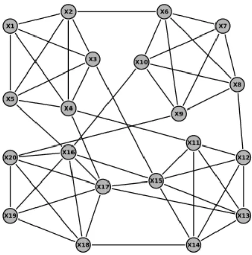
Figure 2.1 – An example of constraint graph

Graph concept is very useful in capturing the structure of a constraint prob-lem. A constraint network can be represented by a graph called a primal constraint

graph, where each vertex represents a variable and the arcs connect all vertices whose variables belong to a constraint scope (see Figure2.1).

Definition 2.7 (Constraint Graph). A constraint graph can be associated with a

con-straint graph G = (V, E), where vertices V represent variables X, and edges E represent constraints C.

2.1.2

Examples of Constraint Networks

In this section, we present some common examples of problems that can be intuitively modeled as constraint networks.

Queens Problem

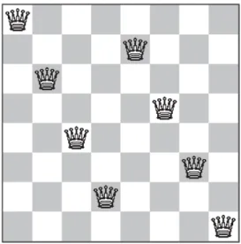
Figure 2.2 – An example of 8-Queens problem

The Description. The classic example used to illustrate a constraint satisfaction

problem is the n-queens problem (see Figure2.2). The problem is to place n queens on a n×nchessboard such that the placement of no queen constitutes an attack on any other.

The Model. One possible constraint network formulation of the problem is as

fol-lows. There is a variable for each column of the chessboard. Variables: X = {x1, . . . , xn};

Domains: D_i= {1,...,n}; Constraints:

— ∀i, j∈{1, . . ., n} xi6= xj(One queen each row.)

2.1 Constraint Programming 15

Graph-coloring Problem

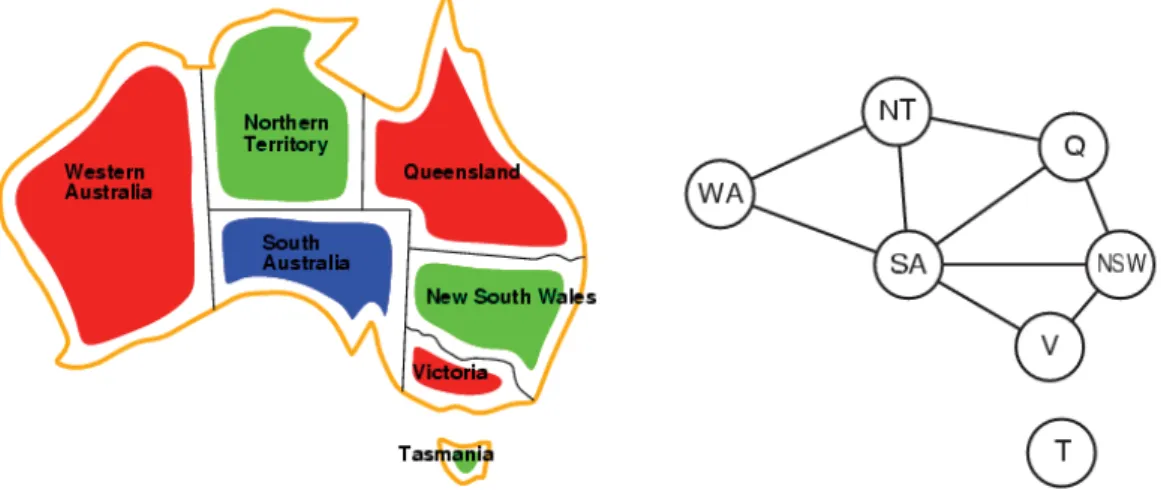
The Description. Another example of constraint network is the graph-coloring

problem. In this problem, the goal is to color the nodes of a graph so that there is not a pair of linked nodes colored with the same color. Each node has a finite number of possible colors. This problem can be modeled as a constraint network by representing each node of the graph as a variable. The domain of each variable is defined by the possible colors that this variable can take. There exits a constraint between each pair of linked variables that forbids these variables to have the same color.

Figure 2.3 – An example of graph-coloring problem

The Model. The graph-coloring problem of Figure2.3is modeled as follows. Variables: X = {WA, NT, Q, NSW, V, SA, T };

Domains: Di= {red,green,blue};

Constraints: adjacent regions must have different colors.

Sudoku Problem

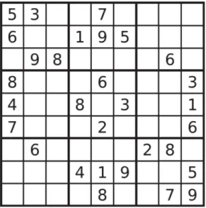
The Description. Sudoku, originally called Number Place, is a logic-based

combi-natorial number-placement puzzle (Figure 2.4). The task is to fill a 9×9 grid with digits so that each column, each row, and each block contains all of the digits from 1 to 9. The puzzle setter provides a partially completed grid, which for a well-posed puzzle has a unique solution.

The Model. The Sudoku puzzle can be modeled as follows.

Variables: X = {x11, . . . , x99};

Domains: D = {D_ij= {1,...,9} |∀i, j∈1, . . . , 9};

Constraints:

— ∀j∈1, . . . , 9 AllDifferent(xij| i∈1, . . . , 9);

— ∀i, j∈1, . . . , 9 AllDifferent(x_(3i+k)(3j+q)| k, q∈1, . . . , 3).

Figure 2.4 – An example of sudoku problem.

2.1.3

Solving Methods

Constraint satisfaction problems are solved using search techniques. The most used techniques are variants of backtracking, constraint propagation, and local search.

Backtracking Search

Backtracking is a recursive algorithm [Knuth, 1968; Rossi et al., 2006b]. It maintains a partial assignment of the variables. Initially, all variables are unas-signed. At each step, a variable is chosen, and all possible values are assigned to it consecutively. For each value, the consistency of the partial assignment with the constraints is checked, and in case of consistency, a recursive call is performed. When all values have been tried, the algorithm backtracks. In this basic backtrack-ing algorithm, consistency is defined as the satisfaction of all constraints whose variables are all assigned. In the literature, several variants of backtracking have been proposed. Backmarking [Gaschnig, 1977] improves the efficiency of check-ing consistency. Backjumpcheck-ing [Prosser, 1993] allows saving part of the search by backtracking “more than one variable” in some cases. Constraint learning [Dechter, 1990] infers and saves new constraints that can be later used to avoid exploring part of the tree search. Look-ahead [Haralick and Elliott,1980] is also often used in

2.2 Constraint Language and Basis 17 backtracking to anticipate the effects of choosing a variable or a value, thus, some-times determining in advance when a subproblem is satisfiable or unsatisfiable.

Propagation

Constraint propagation techniques are methods used to modify the structure of a constraint satisfaction problem [Bessiere,2006]. More accurately, they are meth-ods that enforce a form of local consistency, which are conditions related to the consistency of a group of variables and/or constraints. Constraint propagation has various uses. First, it change a problem into equivalent one, which is usually sim-pler to solve. Second, it may prove satisfiability or unsatisfiability of problems. This is not guaranteed to happen in general; however, it always happens for some forms of constraint propagation and for some certain kinds of problems. The most used form of local consistency are arc consistency, hyper-arc consistency, and path con-sistency. The most popular constraint propagation method is the AC − 3 algorithm [Mackworth,1977], which enforces arc consistency.

Local search

Local search methods [Hoos and Tsang,2006] are incomplete satisfiability algo-rithms. They may find a solution of a problem, but they may fail even if the problem has a solution. They work by iteratively improving a complete assignment over the variables. At each step, it changes the values of some variables, with the over-all purpose of increasing the number of constraints satisfied by this assignment. based in that principle, the min-conflicts algorithm [Minton et al., 1992] is a local search algorithm dedicated for solving CSPs. In practice, local search appears to work well when these changes are also affected by random choices. Integration of backtracking search with local search has been developed, leading to hybrid algo-rithms [Wallace and Schimpf,2002].

2.2

Constraint Language and Basis

In this section, we present two essential components for the constraint acquisi-tion problem, which are constraint language and basis. A constraint language is a set of relations that restricts the type of constraints that are allowed when modeling a constraint satisfaction problem as a constraint network.

Definition 2.8 (Constraint Language). A constraint language is a set Γ = {r1, . . . , rt} of t relations over some subset ofZ.

We are now ready to define the basis for the constraint acquisition problem. The basis is the set of all possible constraints that are candidate for being in the target constraint network.

Definition 2.9 (Basis). Given a vocabulary (X,D) and a constraint language Γ . The

basis for the constraint acquisition problem is the set B of all constraints c for which var(c) is a sequence of variables of X, and there exists a relation r_i in Γ such that rel(c) = ri∩D|var(c)|.

It is worth to notice that the building of a basis B using a constraint language of bounded arity k is polynomial in the input dimension; the size of B is bounded by nkt in the general case, and by n2t _{in the case of binary constraint networks. However,} if Γ contains global constraints, th size of B is no longer polynomial; as one global constraint gives rise to 2n_{possible constraints in B.}

Example 2.1. Consider the binary constraint language Γ = {6=,≥,≤} overZ. Given the vocabulary defined by X = {x1, x2, x3} and D = {1, 2, 3, 4}, we observe that the constraint network C = {6=₁₂,≥₁₂,≤₂₃} is indeed a subset of the basis B = {6=₁₂,≥₁₂,≤₁₂,6=₁₃,≥₁₃,≤₁₃

,6=₂₃,≥₂₃,≤₂₃}.

2.3

Concept Learning

Inducing general functions from specific training examples is a main issue of machine learning [Mitchell,1997]. Concept Learning consists on acquiring the def-inition of a general concept from positive and negative training examples of the target concept. Concept Learning can be seen as a problem of searching through a predefined space of potential hypotheses for the hypothesis that is consistent with the training examples. The hypothesis space has a general-to-specific ordering of hypotheses, and the search can be efficiently organized by taking advantage of a naturally occurring structure over the hypothesis space.

In our setting, which is acquiring constraints from examples, a general concept is a Boolean function over DX_{= Πx}

i∈XD(xi); that is, a map that assigns to each example

e∈DXa value in {0,1}. A representation of a general concept f is a constraint network Cfor which f−1_{(1) = sol(C). A general concept f is said to be representable by a basis} Bif there is a subset C of B such that C is a representation of f. We call target concept the concept fT that returns 1 for e if and only if e is a solution of the problem the user has in mind. The target concept is represented by a target constraint network denoted by CT.

Definition 2.10 (Membership query). A membership query Ask(e), with var(e)⊆X, is a classification question asked to the user, where e is an assignment in Dvar(e)= Π_xi∈var(e)D(xi). A set of constraints Caccepts an assignment e if and only if there does not exist any constraint c∈C rejecting e. The answer to Ask(e) isyes if and only if CT accepts e.

2.4

Constraint Acquisition

In Constraint Programming, it is well known that the modeling task is a bot-tleneck [Freuder,1999; Puget,2004]. This bottleneck has a negative effect on the

2.4 Constraint Acquisition 19 uptake of CP technology on a large scale, especially in the industrial field. An an-swer to the modeling task is constraint acquisition, which lies in the conjunction of two research areas, namely Constraint Programming and Machine Learning. The idea behind that is to assist a non-expert user in modeling her problem as a con-straint network. Several concon-straint acquisition systems have been proposed in the last decade; we will survey the existing systems in the following section. In this section, we formally define constraint acquisition.

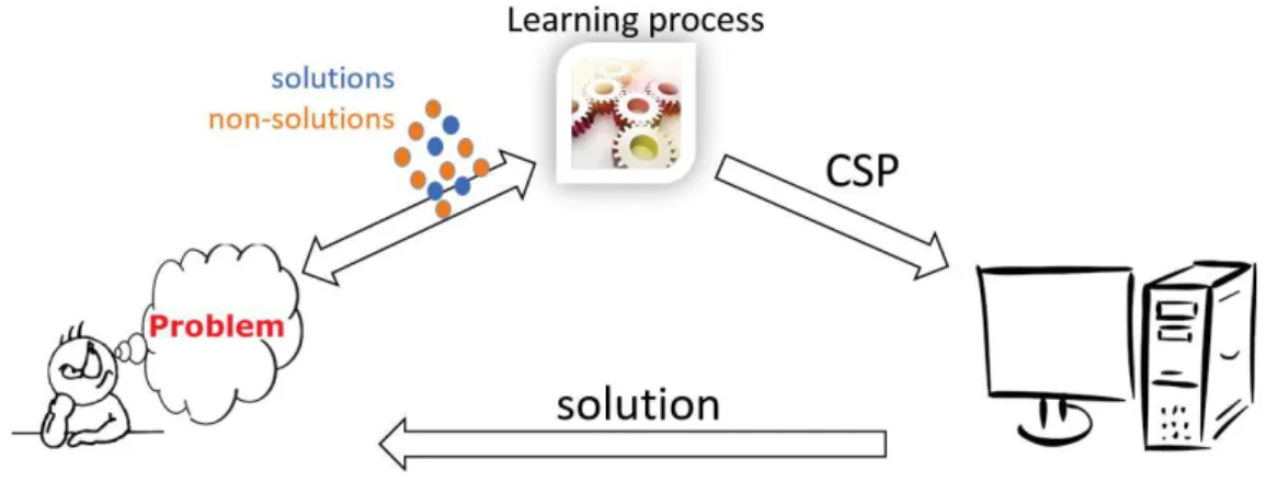
Figure 2.5 – Constraint acquisition.

Constraint acquisition can be seen as an interplay between the user and the learner (see Figure2.5). The learner has a combinatorial problem in her mind, noted CT. We suppose that the common knowledge between the user and the learner is the vocabulary (X,D). In one hand, the user has in her disposal a set of examples that represent both solutions and non-solutions of her problem. In the other hand, the learner owns a library of constraints L and a basis B that we suppose capturing the problem of the user. The objective of the learner is to induce a constraint network CLthat best fits the training examples proposed by the user, and which is equivalent to CT (i.e, CL≡CT). That is, a constraint network that accepts the positive examples and rejects the negative ones.

In the literature, there are two forms of constraint acquisition. The first form is a passive learning, and the second form is an active learning.

2.4.1

Passive Learning

In a passive constraint acquisition context, there is no interplay between the user and the learner. The user provides a set of positive and negative examples, and the learner tries to find a set of constraints that classifies the training examples.

Definition 2.11 (Passive constraint acquisition problem). Given a vocabulary (X,D),

solu-tions E+, and an other set of non-solutions E−of the problem the user has in mind, the constraint acquisition problem is, therefore, to find C such that:

— C⊆B

— For each e∈E+, e satisfies all constraints in C

— For each e∈E−, e rejected by at least one constraint in C

2.4.2

Active Learning

By contrast, in an active setting, the user dialogs with the learner. The learner proposes informative examples, and the user classifies them as positive or negative. The benefit of such kind of learning is that it provides less of a burden on the user.

Definition 2.12 (Active constraint acquisition problem). Given a basis B and an

unknown user classification function f, the active constraint acquisition problem is to find a converging sequence Q = {q₁, . . . , qm} of queries. That is, a sequence such that qi+1is a query relative to B and CL, where CLis the constraint network learned so far, i.e the learned constraint network after classifying qi. After the classification of the query qm, the learner converges on the target constraint network, i.e CL≡CT.

The general context underlying this thesis is the active constraint acquisition. Our objective is to make this kind of learning more efficient in practice despite the context of use.

2.4.3

Constraint Acquisition as a Search

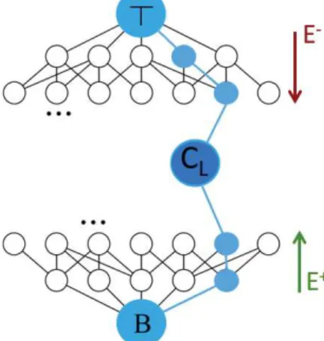
Constraint acquisition can be seen as a form of search through a search space. The search space can be represented as a lattice (see Figure 2.6). Each node of the lattice is a possible constraint network. The top ⊤ of the lattice represents

the general constraint network, which accepts all examples provided by the user. The specific born of the lattice is represented by all constraints of the basis B. The search space is explored via examples classified by the user. In the case of a positive example, we prune the search space by removing all constraints that reject the example. Hence, we generalize our learned constraint network, and we then go up through the lattice. In the case of a negative example, we learn at least one constraint that explains the rejection of that example. That is, we specify our learned constraint network, by going dawn through the lattice.

2.5

Existing Constraint Acquisition Systems

In this section, we survey the existing constraint acquisition systems proposed in the last years.

2.5 Existing Constraint Acquisition Systems 21

Figure 2.6 – Search space in constraint acquisition

2.5.1

C

.1

CONACQ.1 is a SAT-based algorithm presented in [Bessiere et al., 2004, 2005] for acquiring constraint networks based on version space [Winston,1992;Mitchell,

1997]. In CONACQ.1, Bessiere et al. made the assumption that the only thing the user is able to provide is examples of solutions and non-solutions of the target problem. Based on these examples, the CONACQ.1 system learns a set of constraints that correctly classifies all examples given so far. This type of learning is called passive learning.

Description of CONACQ.1

The set of the training examples provided to CONACQ.1 by the user is composed of negative and positive examples.

Definition 2.13 (Training Data). The set Ef _{of training examples provided to} CONACQ.1 is composed of a set E of instances and a classification function f : E−→ {0, 1}. Given an element e of E, f(e) = 1 if and only if e is a solution of the problem that the user has in mind. That is, e is a positive example noted e+. If e is a non-solution of the problem, therefore, f(e) = 0, and we say that the example is negative, noted e−.

We say that a constraint network C is consistent with the training data Ef_{if and} only if each example e+_∈Ef _{belongs to the set of solutions of C, and each e}−_∈Ef _is a non-solution of C. Given a basis B and a set of training data Ef_{, the problem of} constraint acquisition consists on finding a constraint network C admissible for B and consistent with the training data Ef_.

CONACQ.1 is a constraint acquisition system based on the version space intro-duced by Mitchel in [Mitchell, 1997]. The version space is a supervised machine

learning technique that aims at acquiring a target concept from positive and nega-tive examples. Formally speaking, given a set of hypotheses H and a set of training examples E, the version space is the set of hypotheses of H that are consistent with the training examples. In the setting of constraint acquisition, the version space VB(Ef), of a constraint acquisition problem, is the set of all constraint networks admissible by B and consistent with the training examples Ef_{. In the SAT-based} for-mulation of CONACQ.1, the version space is encoded by the clausal theory K, where each model of this theory is a constraint network of VB(Ef).

If B is the basis, a literal is either an atom bijof B or its negation ¬bij. It is wroth to stress that ¬bij is not a constraint, but it point out that bij does not belong to the learned constraint network. A clause is a disjunction of literals, and the clausal theory K is a conjunction of clauses.

Definition 2.14 (Interpretation). Let B be a basis. An interpretation I over B is a

function that assigns to each literal bijin B a value I(bij) in {0,1}

Definition 2.15 (Transformation). Let B be a basis. A transformation is a function φ

that assigns to each interpretation I of B the constraint network φ(I) admissible by B and such that:

C_ij∈φ(I) iff C_ij=T{bp_ij∈B | I(bp_ij) = 1}

An interpretation I is a model of the clausal theory K if K is true in I according to the standard propositional semantic. The set of all the models of K is noted Models(K).

The construction of K is as follows. For each training example e provided by the user, CONACQ.1 builds the set k(e), of literals corresponding to the constraints bij∈B, that rejects e. Then, CONACQ.1 adds iteratively a set of clauses such that, for each interpretation I of Models(K), the network φ(I) classifies correctly the the training examples given so far, as well as the example e. The update of the clausal theory differs according to the learning class of e:

— If e is a negative example, then one of the constraints in k(e) explains the rejection of e. We then add to K the disjunction {W_bij∈k(e)bij}of elements of k(e). — If e is a positive example, then CONACQ.1 is ensured that no one of the con-straints of k(e) belongs to the target network. Consequently, K is updated by adding the conjunction of the unitary clauses ¬bijof k(e).

The analysis of positive instances of Ef _{allows to simplify, with unitary} propaga-tion, the clauses that explain the rejection of negative examples. The correction of the algorithm CONACQ.1 is formulated by the theorem2.1.

Theorem 2.1 (Correctness of CONACQ.1). Let Ef_{be a set of training examples and B} a basis. The clausal theory built byCONACQ.1 for Ef_{and B is such that:}

2.5 Existing Constraint Acquisition Systems 23

Proof. The proof of the theorem 2.1is given in [Bessiere et al.,2005].

CONACQ.1 has numerous advantages. Firstly, the formulation is generic; there-fore, it can use any SAT solver as a basis for version space learning. Secondly, it can exploit powerful SAT concepts, such as unit propagation and backbone detection to improve learning rate. Finally, CONACQ.1 can easily incorporate domain-specific knowledge in constraint programming to improve the quality of the learned net-work. Specifically, for handling redundant constraints in constraint acquisition, two generic techniques have been developed. The first is based on the notion of redundancy rules, which can deal with some forms of redundancy. The second technique, based on backbone detection, is far more powerful.

Despite its distinct number of advantages, CONACQ.1 has also some limitations. Firstly, It cannot acquire global constraints. Secondly, it may require a number exponential of examples to get the target network [Bessiere and Koriche,February, 2012]. Thirdly, and finally, CONACQ.1 needs positive examples to learn constraints; why modeling a problem if we have already, at our disposal, solutions for it?

2.5.2

C

.2

To overcome the limitations reproached to CONACQ.1, Bessiere et al. have pro-posed an active learning version, called CONACQ.2 [Bessiere et al., 2007]. The system CONACQ.2 proposes examples to the user to classify as solutions or non-solutions. Such questions are called membership queries [Angluin,1987].

Description of CONACQ.2

In order to generate queries, the authors proposed several approaches. First, a random affectation to the variables, which is a baseline approach. Second, a query with a small K(e). Finally, a query with a large k(e). It is worth to notice that using these approaches could generate useless queries. In fact, a query does not contain information if it is rejected by the version space. We then talk about redundant queries.

Definition 2.16 (A redundant query). A redundant query is a query that do not allow

us to learn new informations. Let e be an example, we have tow cases of redundant queries:

— Either k(e) = ∅ and in this case we automatically detect that e is a solution; — Or all constraints rejecting e are already in K; then, any constraint network in

the version space accepts e.

Hence, redundant queries are useless, and it is not necessary asking the user to classify them.

To make CONACQ.2 more efficient in terms of number of queries, the authors propose some optimizations. They propose to break some clauses of K. That is, they propose to compute a query with k(e) containing a strict subset of literals present in

the clause that they wish to break. If this query is classified as negative, they get a smaller clause that contains only literals existing in k(e). Otherwise, they decrease the size of the clause by setting all literals of k(e) to false. Note that if one seeks a query with a k(e) of size 1, and if the query is classified by the user as negative; then, the clause will be simplified to a single variable, which must therefore be true. The last optimization, proposed by the authors, concerns a case occurring if they try to break clauses. This case arises when they force the not fixed variables to be true in order to such variables do not appear in k(e). In this case, it is possible that no query exists. They propose to extract a conflict set S of literals and to add the clauseWbij∈S¬bij forcing at least one of the variables to be false. In practice, there

are several methods to produce such conflict sets. One method is, for each variable bij∈k(e), to test whether to fix it to true; then, K becomes inconsistent. In this case, this variable must be false.

Even that CONACQ.2 is active and generates only informative examples, it re-mains exponentially large in terms of number of queries; it may require a large number of queries to get the target constraint network. Thus, it is hard to put CONACQ.2 in practice. An other weakness of CONACQ.2 is that it is not able to learn global constraints that are not decomposable.

2.5.3

M

S

In [Beldiceanu and Simonis, 2012], Beldiceanu and Simonis proposed Model Seeker, another passive learning approach. Positive examples are provided by the user. The system arranges these examples as a matrix, or any other data structure, and identifies constraints in the global constraints catalog ([Beldiceanu et al.,2007]) that are satisfied by rows or columns of all examples.

Description of MODELSEEKER

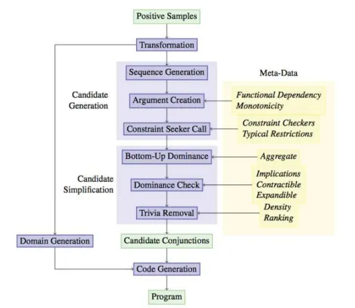
The general schema of MODELSEEKERis shown in Figure2.7. Here, we will give a general overview of the different steps of the system. MODELSEEKER takes as input positive examples of the problem that we want to model as a constraint network.

Transformation In the first step, MODELSEEKER tries to convert the format of in-put examples to other more appropriate representations. For instance, it tries to replace a boolean format with finite domain values. MODELSEEKER also converts different graph representations into the successor variable form used by the global constraints in the catalog.

Candidate Generation The second step (Sequence Generation) tries to group the

variables of the example into regular subsets. For instance, it interprets the input vector as a matrix and creates subsequences for all rows and all columns. In the Ar-gument Creationstep, MODELSEEKER creates call patterns for constraints from the subsequences. it can try each subsequence on its own, or combine pairs of subse-quences, or use all subsequences together in a single collection. It also tries to add additional arguments based on functional dependencies of constraints, described

2.5 Existing Constraint Acquisition Systems 25

Figure 2.7 – General schema of MODELSEEKER.

as meta-data in the global constraint catalog. For each call pattern, MODELSEEKER then calls the Constraint Seeker to discover matching constraints, which satisfy all subsequences of each example. Only the highest ranking candidates are retained for further analysis.

Candidate Simplification After the Constraint Seeker step, MODELSEEKER poten-tially has a very large list of possible candidate global constraints (up to 2 000 global constraints for some examples). The next step is to reduce this list as much as pos-sible. first, MODELSEEKERapplies a Dominance Check to remove all candidate con-straints that are implied by other concon-straints in the candidate list. The dominance check is the core of modeling system, helping to remove useless constraints from the candidate list. In the last step before the final candidate list output, the system removes trivial constraintsand simplifies some constraint pattern. At the end of this step, MODELSEEKERperforms a ranking of the remaining candidates based on the constraint and sequence generator used.

Code Generation As a side effect of the initial transformation in the first step,

consideration. In the default case, the system just creates variable domains using all values occurring in the examples. But, for some graph-based transformations a more accurate domain definition is used. At the last step, which is Code Generation, given the candidate list and domains for the variables, It can be easily to generate code for a model using the constraints. MODELSEEKER produces SICStus Prolog code using the call format of the catalog. The generated code can then be used to validate the provided examples or to find solutions for the learned constraint network.

MODELSEEKER remains the only system that deals with global constraints. The major drawback of MODELSEEKER is that it does not handle all global constraints in the catalog [Beldiceanu et al., 2007]. It deals only with 67 global constraints. Another reproach to that system is that it learns only from positive examples; hence, it makes the system hard to put in practice, as the provide of such examples by a novice is not an obvious task.

2.5.4

Q

A

QUACQ is a recent active learner system that is able to ask the user to classify partial queries [Bessiere et al., 2013]. Using partial queries and given a negative example, QUACQ is able to find a constraint of the problem the user has in mind in a number of queries logarithmic in the size of the example. This key component of QUACQ allows it to always converge on the target set of constraints in a polynomial number of queries. However, even that good theoretical bound can be hard to put in practice. For instance, QUACQ requires the user to classify more than 8000 examples to get the complete Sudoku model.

Description of QUACQ

QUACQ takes as input a basis B on a vocabulary (X,D). It asks partial queries of the user until it has converged on a constraint network CL equivalent to the target network CT, or collapses. When a query is answered yes, constraints rejecting it are removed from B. When a query is answered no, QUACQenters a loop (functions FindScopeand FindC) that will end by the addition of a constraint to CL.

QUACQ (see Algorithm 1) initializes the network CL it will learn to the empty set (line 2). If CL is unsatisfiable (line 6), the space of possible networks collapses because there does not exist any subset of the given basis B that is able to correctly classify the examples already asked of the user. In line 8, QUACQ computes a complete assignment e satisfying CL but violating at least one constraint from B. If such an example does not exist (line 10), then all constraints in B are implied by CL, and we have converged. If we have not converged, we propose the example e to the user, who will answer by yes or no. If the answer is yes, we can remove from B the set κB(e)of all constraints in B that reject e (line12). If the answer is no, we are sure that e violates at least one constraint of the target network CT. We then call the function FindScope to discover the scope S of one of these violated constraints (line

2.5 Existing Constraint Acquisition Systems 27

Algorithm 1: QUACQ: Acquiring a constraint network CT with partial queries 1 CL← ∅;

2 while true do

3 if sol(CL) = ∅ then return “collapse”;

4 choose e in DXaccepted by C_L and rejected by B ; 5 if e = nil then return “convergence on CL”; 6 if ASK(e) = yes then B ← B \ κ_B(e);

7 else

8 _{S ← FindScope(e,∅,X,false);} 9 c_{S← FindC(S);}

10 if cS= nil then return “collapse”; 11 else C_{L← CL}∪{cS};

20). FindC will return a constraint of CT whose scope is in S (line9). If no constraint is returned (line 22), this is again a condition for collapsing as we could not find in B a constraint rejecting one of the negative examples. Otherwise, the constraint returned by FindC is added to the learned network CL (line28).

The recursive function FindScope (see Algorithm2) takes as parameters an ex-ample e, two sets R and Y of variables, and a Boolean ask_query. An invariant of FindScopeis that e violates at least one constraint whose scope is a subset of R∪Y. When FindScope is called with ask_query = false, we already know whether R con-tains the scope of a constraint that rejects e (line 3). If ask_qery = true we ask the user whether e[R] is positive or not (line4). If yes, we can remove all the constraints that reject e[R] from the basis, otherwise we return the empty set (line5). We reach line6only in case e[R] does not violate any constraint. We know that e[R∪Y]violates a constraint. Hence, as Y is a singleton, the variable it contains necessarily belongs to the scope of a constraint that violates e[R∪Y]. The function returns Y. If none

of the return conditions are satisfied, the set Y is split in two balanced parts (line 7) and we apply a technique similar to QUICKXPLAIN ([Junker,2004a]) to elucidate the variables of a constraint violating e[R∪Y]in a logarithmic number of steps (lines 8–10).

The function FindC (see Algorithm3) takes as parameter Y, the scope on which FindScopehas found that there is a constraint from the target network CT. FindC first removes from B all constraints with scope Y that are implied by CL because there is no need to learn them (line 3). The set ∆ is initialized to all candidate constraints (line 4). In line6, an example e is chosen in such a way that ∆ contains both constraints rejecting e and constraints satisfying e. If no such example exists (line 7), this means that all constraints in ∆ are equivalent wrt CL[Y]. Any of them is returned except if ∆ is empty (lines 8-9). If a suitable example was found, it is proposed to the user for classification (line10). If classified positive, all constraints rejecting it are removed from B and ∆ (line 11). Otherwise we test whether the

Algorithm 2: Function FindScope: returns the scope of a constraint in CT 1 function FindScope(in e: example, R,Y: scopes, ask_query: Boolean): scope; 2 begin

3 if ask_query then

4 if ASK(e[R]) = yes then B ← B \ κB(e[R]); 5 else return ∅;

6 if |Y| = 1 then return Y;

7 split Y into<Y1, Y2>such that |Y1|=⌈|Y|/2⌉; 8 S1← FindScope(e,R∪Y1, Y2,true);

9 S2← FindScope(e,R∪S1, Y1, (S16= ∅)); 10 return S1∪S2;

Algorithm 3: Function FindC: returns a constraint of CT with scope Y 1 function FindC(in Y: scope): constraints;

2 begin

3 B ← B \ {cY| CL|= cY}; 4 _{∆ ← {cY}|(c_Y∈B[Y]);

5 while true do

6 choose e in sol(C_L[Y])such that ∃cY, c_Y′ ∈∆, e |= cY and e6|= c_Y′; 7 if e = nil then

8 if ∆ = ∅ then return nil; 9 else pick cY in ∆; return c; 10 if ASK(e) = yes then

11 _{B ← B \ κB}(e); ∆ ← ∆\κB(e);

12 else

13 if∃cS∈κB(e) | S ( Y then

14 return FindC(FindScope(e,∅,Y,false)); 15 else ∆ ← ∆∩κB(e);

example e does not violate constraints with scope strictly included in Y (line13). If yes, we recursively call FindScope and FindC to find that smaller arity constraint before the one having scope Y (line 14). If no, we remove from ∆ all constraints accepting that example e (line15) and we continue the loop of line5.

Complexity of QUACQ

The complexity of QUACQ, in terms of queries, is given by Theorem2.2.

2.5 Existing Constraint Acquisition Systems 29 constraints, and a target network CT, QUACQ uses O(CT.(log|X| + |Γ|)) queries to find the target network or to collapse and O(|B|) queries to prove convergence.

Proof. The proof of the theorem 2.2is given in [Bessiere et al.,2013].

Illustrative Example

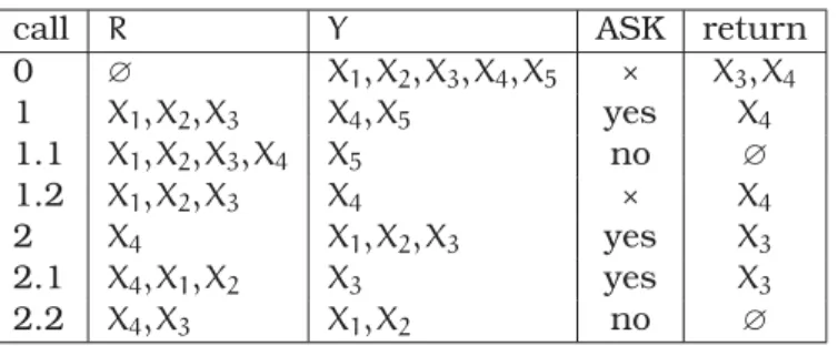
Table 2.1 – The example

call R Y ASK return

0 ∅ X1, X2, X3, X4, X5 × X3, X4 1 X1, X2, X3 X4, X5 yes X4 1.1 X1, X2, X3, X4 X5 no ∅ 1.2 X1, X2, X3 X4 × X4 2 X4 X1, X2, X3 yes X3 2.1 X4, X1, X2 X3 yes X3 2.2 X4, X3 X1, X2 no ∅

We illustrate the behavior of QUACQ on a simple example. Consider the set of variables X1, . . . , X5 with domains {1..5}, a language Γ = {=,6=}, a basis B = {=ij ,6=ij| i, j∈1..5, i<j}, and a target network CT = {=15, 6=34}. Suppose the first exam-ple generated in line 8 of QUACQ is e1= (1,1,1,1,1). The trace of the execution of FindScope(e1, ∅, X1. . . X5,false) is in Table 2.1. Each line corresponds to a call to FindScope. Queries are always on the variables in R. ’×’ in the column ASK means

that the previous call returned ∅, so the question is skipped. The queries in lines 1 and 2.1 in the table permit FindScope to remove the constraints6=12,6=13,6=23 and

6

=₁₄,6=₂₄from B. Once the scope (X3, X4)is returned, FindC requires a single example to return6=₃₄and prune =34from B. Suppose the next example generated by QUACQ is e2= (1,2,3,4,5). FindScope will find the scope (X1, X5) and FindC will return =15 in a way similar to the processing of e1. The constraints =12, =13, =14, =23, =24 are removed from B by a partial positive query on X1, . . . , X4 and 6=15 by FindC. Finally, examples e3= (1,1,1,2,1) and e4= (3,2,2,3,3), both positive, will prune 6=25,6=35, =45 and =25, =35,6=45 from B respectively, leading to convergence.

C

3

Constraint Acquisition with

Generalization Queries

Preamble

In this chapter, we introduce the concept of generalization query based on an aggregation of variables into types. We present a constraint generalization al-gorithm that can be plugged into any constraint acquisition system. We propose several strategies to make our approach more efficient in terms of number of queries. Finally we experimentally compare the recent QUACQ system to an extended version boosted by the use of our generalization functionality. The results show that the extended version dramatically improves the basicQUACQ.

Contents

3.1

Introduction

Constraint programming (CP) is used to model and to solve combinatorial prob-lems in many application areas, such as resource allocation or scheduling. However, building a CP model requires some expertise in constraint programming. This pre-vents the use of this technology by a novice and thus this has a negative effect on the uptake of constraint technology by non-experts.

Several techniques have been proposed for assisting the user in the modeling task. In [Freuder and Wallace, 2002], Freuder and Wallace proposed the

match-maker agent, an interactive process where the user is able to provide one of the constraints of her target problem each time the system proposes a wrong solution. In [Lallouet et al.,2010], Lallouet et al. proposed a system based on inductive logic programming that uses background knowledge on the structure of the problem to learn a representation of the problem correctly classifying the examples. In [Bessiere et al.,2004,2005], Bessiere et al. made the assumption that the only thing the user is able to provide is examples of solutions and non-solutions of the target problem. Based on these examples, the Conacq.1 system learns a set of constraints that cor-rectly classifies all examples given so far. This type of learning is called passive learning. In [Beldiceanu and Simonis, 2012], Beldiceanu and Simonis proposed Model Seeker, another passive learning approach. Positive examples are provided by the user. The system arranges these examples as a matrix and identifies con-straints in the global concon-straints catalog ([Beldiceanu et al.,2007]) that are satisfied by rows or columns of all examples.

By contrast, in an active learner like Conacq.2, the system proposes examples to the user to classify as solutions or non solutions [Bessiere et al., 2007]. Such questions are called membership queries [Angluin, 1987]. CONACQ introduces two computational challenges. First, how does the system generate a useful query? Second, how many queries are needed for the system to converge to the target set of constraints? It has been shown that the number of membership queries required to converge to the target set of constraints can be exponentially large [Bessiere and Koriche,February, 2012].

QUACQ is a recent active learner system that is able to ask the user to classify partial queries [Bessiere et al., 2013]. Using partial queries and given a negative example, QUACQ is able to find a constraint of the problem the user has in mind in a number of queries logarithmic in the size of the example. This key component of QUACQ allows it to always converge on the target set of constraints in a polynomial number of queries. However, even that good theoretical bound can be hard to put in practice. For instance, QUACQ requires the user to classify more than 8000 examples to get the complete Sudoku model.

In this chapter, we propose a new technique to make constraint acquisition more efficient in practice by using variable types. In real problems, variables often repre-sent components of the problem that can be classified in various types. For instance, in a school time-tabling problem, variables can represent teachers, students, rooms, courses, or time-slots. Such types are often known by the user. To deal with types of variables, we introduce a new kind of query, namely, generalization query. We expect the user to be able to decide if a learned constraint can be generalized to other scopes of variables of the same type as those in the learned constraint. We propose an algorithm, GENACQ for generalized acquisition, that asks such general-ization queries each time a new constraint is learned. We propose several strategies and heuristics to select the good candidate generalization query. We plugged our generalization functionality into the QUACQ constraint acquisition system, leading to theG-QUACQalgorithm. We experimentally evaluate the benefit of our technique

3.2 GENACQAlgorithm 33 on several benchmark problems. The results show that G-QUACQ dramatically im-proves the basic QUACQ algorithm in terms of number of queries.

The rest of this chapter is organized as follows. Section Section 3.2 describes the generalization algorithm. In Section 3.3, several strategies are presented to make our approach more efficient. Section3.4presents the experimental results we obtained when comparing G-QUACQ to the basic QUACQ and when comparing the different strategies in G-QUACQ. Section3.5concludes the chapter and gives some directions for future research.

3.2

G

A

Algorithm

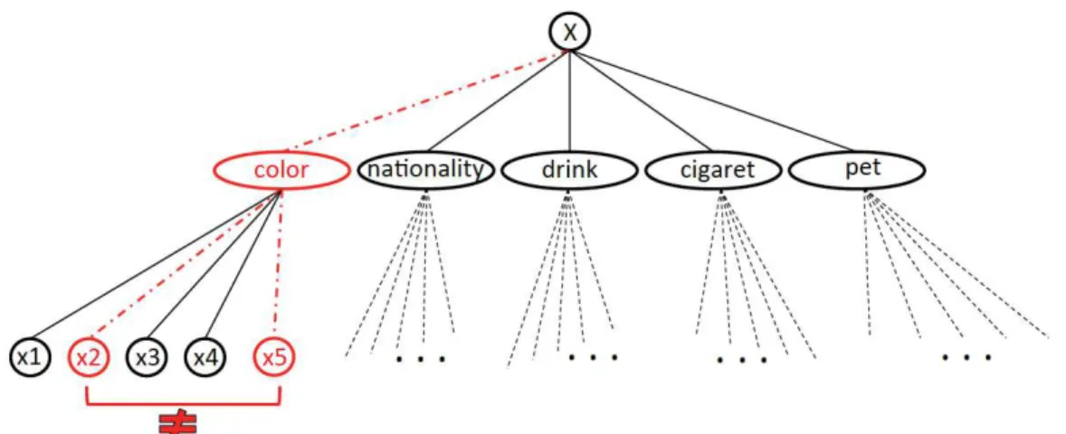
In this section we present GENACQ, a generalized acquisition algorithm, The idea behind this algorithm is, given a constraint c learned on var(c), to generalize this constraint to sequences of types s covering var(c) by asking generalization queries AskGen(s, r). A generalization query AskGen(s,r) is answered yes by the user if and only if for every sequence var of variables covered by s the relation r holds on var in the target constraint network CT.

Algorithm 4: GENACQ (c,NonTarget) 2

2 Table ← {s | var(c)∈s} \ {var(c)} 4 4 _{G ← ∅} 6 6 #NoAnswers ← 0 8 8 foreach s∈Table do 10 10 if ∃(s′_{, r)∈NegativeQ | rel(c)⊆} r∧s′_⊑sthen 12 12 Table ← Table \ {s} 14 14 if ∃c′_{∈NonTarget | rel(c}′ ) = rel(c)∧var(c′_)∈sthen 15 Table ← Table \ {s} ; 17

17 while Table6_{= ∅ ∧ #NoAnswers}<cutoffNo do 19

19 pick s in Table 21

21 if AskGen(s,rel(c)) = yes then 23

23 G ← G∪{s} \ {s′_{∈G | s}′_⊑s} 25

25 _{Table ← Table \ {s}′∈Table | s′_⊑s} 27

27 #NoAnswers ← 0 28 else

30

30 Table ← Table \ {s′∈Table | s⊑s′_} 32

32 _{NegativeQ ← NegativeQ}∪{(s,rel(c))} 34

34 #NoAnswers + + 36

3.2.1

Description of G

A

The algorithm GENACQ (see Algorithm 4) takes as input a target constraint c that has already been learned and a set NonTarget of constraints that are known not to belong to the target network. It also uses the global data structure NegativeQ, which is a set of pairs (s,r) for which we know that r does not hold on all sequences of variables covered by s. c and NonTarget can come from any constraint acquisition mechanism or as background knowledge. NegativeQ is built incrementally by each call to GENACQ. GENACQ also uses the set Table as local data structure. Table will contain all sequences of types that are candidates for generalizing c.

In line 2, GENACQ initializes the set Table to all possible sequences s of types that contain var(c). In line3, GENACQ initializes the set G to the empty set. G will contain the output of GENACQ, that is, the set of maximal sequences from Table on which rel(c) holds. The counter #NoAnswers counts the number of consecutive times generalization queries have been classified negative by the user. It is initialized to zero (line 6). #NoAnswers is not used in the basic version of GENACQ but it will be used in the version with cutoffs. (In other words, the basic version uses cutoffNo = +∞ in line17).

The first loop in GENACQ (line8) eliminates from Table all sequences s for which we already know the answer to the query AskGen(s,rel(c)). In lines10-12, GENACQ eliminates from Table all sequences s such that a relation r entailed by rel(c) is already known not to hold on a sequence s′_{covered by s (i.e., (s}′

, r)is in NegativeQ). This is safe to remove such sequences because the absence of r on some scope in s′_{implies the absence of rel(c) on some scope in s (see Lemma3.1). In lines 14-15,} GENACQ eliminates from Table all sequences s such that we know from NonTarget that there exists a scope var in s such that (var,rel(c))∉CT.

In the main loop of GENACQ (line 17), we pick a sequence s from Table at each iteration and we ask a generalization query to the user (line 21). If the user says yes, s is a sequence on which rel(c) holds. We put s in G and remove from G all sequences covered by s, so as to keep only the maximal ones (line 23). We also remove from Table all sequences s′_{covered by s (line 25) to avoid asking redundant} questions later. If the user says no, we remove from Table all sequences s′_{that cover} s(line30) because we know they are no longer candidate for generalization of rel(c) and we store in NegativeQ the fact that (s,rel(c)) has been answered no. The loop finishes when Table is empty and we return G (line16).

3.2.2

Completeness and Complexity

We analyze the completeness and complexity of GENACQ in terms of number of generalization queries.

Lemma 3.1. If AskGen(s,r) = no then for any (s′_{, r}′_{) such that s⊑s}′ _{and r}′_{⊆r, we} have AskGen(s′