HAL Id: hal-00979804
https://hal.inria.fr/hal-00979804
Submitted on 17 Apr 2014
HAL is a multi-disciplinary open access
archive for the deposit and dissemination of
sci-entific research documents, whether they are
pub-lished or not. The documents may come from
L’archive ouverte pluridisciplinaire HAL, est
destinée au dépôt et à la diffusion de documents
scientifiques de niveau recherche, publiés ou non,
émanant des établissements d’enseignement et de
Patterns
Elias Egho, Chedy Raïssi, Nicolas Jay, Amedeo Napoli
To cite this version:
Elias Egho, Chedy Raïssi, Nicolas Jay, Amedeo Napoli. Mining Heterogeneous Multidimensional
Sequential Patterns. [Research Report] RR-8521, INRIA. 2014. �hal-00979804�
ISSN 0249-6399 ISRN INRIA/RR--8521--FR+ENG
RESEARCH
REPORT
N° 8521
April 2014 Project-Teams OrpailleurMining Heterogeneous
Multidimensional
Sequential Patterns
RESEARCH CENTRE NANCY – GRAND EST 615 rue du Jardin Botanique CS20101
54603 Villers-lès-Nancy Cedex
Mining Heterogeneous Multidimensional
Sequential Patterns
Elias Egho
˚, Chedy Raïssi
˚, Nicolas Jay
˚, Amedeo Napoli
˚Project-Teams Orpailleur
Research Report n° 8521 — April 2014 — 25 pages
Abstract: All domains of science and technology produce large and heterogeneous data. Although much work has been done in this area, mining such data is still a challenge. No previous research targets the mining of heterogeneous multidimensional sequential data. In this work, we present a new approach to extract heterogeneous multidimensional sequential patterns with different levels of granularity by relying on external taxonomies. We show the efficiency and interest of our approach with the analysis of trajectories of care for colorectal cancer using data from the French casemix information system.
Key-words: multidimensional sequential patterns, data mining, heterogeneous sequential data
Séquentielles Multidimensionnelles et Hétérogènes
Résumé : Tous les domaines de la science et de la technologie produisent gros volumes de don-nées hétérogènes. L’exploration de tels volumes de dondon-nées reste toujours un défi. Peu de travaux ciblent l’exploration et l’analyse de données séquentielles multidimensionnelles et hétérogènes. Dans ce travail, nous présentons une nouvelle approche appeléeMMISP pour extraire des motifs séquentiels à partir de données séquentielles multidimensionnelles et hétérogènes, selon différents niveaux de granularité dépendant de connaissances extérnes. L’approache MMISP a été ap-pliquée à l’analyser de trajectoires de soins de santé de patients en oncologie. Les données proviennent d’une base de données médico-administrative incluant toutes les informations sur les hospitalisations des patients dans la région Lorraine (France).
Mots-clés : motifs séquentiels multidimensionnels, fouille de données, données hétérogènes séquentielles
Mining Heterogeneous Multidimensional Sequential Patterns 3
1
Introduction
Sequential pattern mining, introduced by Agrawal et al [1], is a popular approach to discover patterns in ordered data. Frequent sequence mining can be seen as an extension of the well known itemset mining problem where the input data is modeled as sequences elements. This method is rather efficient to discover rules of the type: “customers frequently first buy DVDs of seasons I, II of Sherlock, then buy within 6 months season III of the same crime drama series". Sequential pattern mining has been successfully used so far in various domains : amino-acids protein sequence analysis [2], web log analysis [3], and music sequences matching [4].
Many efficient approaches were developed to mine patterns depending on time or order where most of them are based on theApriori property [1], which states that any super pattern of a non-frequent pattern cannot be non-frequent. The main algorithms areGSP [5], SPADE [6], PrefixSpan [7] andClosSpan [8]. However, these techniques and algorithms focus solely on one-dimensional aspect of sequential databases and do not deal with the multidimensional aspect where items can be of different types and described over different levels of granularity. For instance, in a real-world retail company, a database or data warehouse holds much more complex information such as article prices, gender of the customers, geolocation of the stores and so on. In addition, articles are usually represented following a hierarchical taxonomy: apples can be either described as fruits, fresh food or food. Pinto et al. [9], Zhang et al. [10] and Yu et al. [11] introduced the notion of multidimensionality in a sequence and proposed several algorithms to mine this type of data without taking into account the different levels of granularity for each dimension. Plantevit et al. [12] introduced M3
SP, an algorithm able to incorporate several dimensions described over different levels of granularity within the sequential pattern mining process. These approaches focus on homogeneous multidimensional sequence where its elements are described simply as vectors of items. By contrast, in modern life sciences [13], a multidimensional sequential data set is often represented as sequences of vectors with elements having different types (i.e., item and itemset). This special feature is in itself a challenge and multidimensionality in sequence mining needs to be carefully taken into account when devising new efficient algorithms.
In our approach, we aim at providing an approach that extract rules such as: “After buying an article from the fruit category from supermarket A, a customer will buy two articles from the Egg and Dairy products and Beverage categories from supermarket B". This example not only combines two dimensions (supermarket and products) which are ordered over time and are represented with different levels of granularity, but it also characterizes them in a different way as a magazine can be considered as an element taking one value (“item”), while a product can take several values (“itemset”). This example shows that each dimension has to be managed in a proper and suitable way. We believe that our work is the first to present a full framework and al-gorithm to mine such multidimensional sequential patterns from heterogeneous multidimensional sequential database.
The main contribution of this report is to generalize the concept of multidimensional sequence by considering heterogeneous multidimensional sequences. The event in a sequence is considered as a vector of items and itemsets, Such multidimensional and heterogeneous patterns have to be mined by adapted and suitable methods. Accordingly, we propose a new method MMISP (Mining Multidimensional Itemsets Sequential Patterns) to extract sequential patterns from het-erogeneous multidimensional sequential database. In addition, the approach is able to take into account background knowledge lying in taxonomies existing for each dimension. As often with enumeration algorithms, mining all possible sequential patterns from a multidimensional sequen-tial database results in a huge amount of patterns which is difficult to be analyzed [14]. To overcome this problem, MMISP mines only the most specific patterns. We report an extensive empirical study on synthetic datasets and qualitative experiments with a dataset consisting of
Patients Trajectories
s1 xpuhp, ca1,tmp111, mp221uq, puhp, ca1,tmp222uq, pghl, r1,tmp221, mp311uqy
s2 xpuhn, ca1,tmp111uq, puhn, ca2,tmp111, mp211uq, pghl, r1,tmp222, mp312uqy
s3 xpuhn, ca3,tmp112, mp211uq, pghl, r2,tmp222, mp311uqy
s4 xpuhp, ca2,tmp112, mp222uq, pghp, r2,tmp221, mp312uq, pghp, r2,tmp221, mp312uqy
Table 1: An example of a database of patient trajectories.
trajectories of cancer patients extracted from French healthcare organizations. The successive hospitalizations of a patient can be expressed as a sequence of heterogeneous multidimensional attributes such as healthcare institution, diagnosis and set of medical procedures. Our goal is to be able to extract patterns describing patient stays along with combinations of procedures over time. This type of pattern is very useful to healthcare professionals to better understand the global behaviour of patients over time and the associated supports.
The remainder of this report is organized as follows, Section 2 introduces the problem state-ment as well as a running example and briefly reviews the preliminaries needed in our develop-ment. MMISP method is described in Section 3. Section 4 presents experimental results from both quantitative and qualitative point of views and Section 5 concludes the paper.
2
Problem Statement
2.1
An introductory example
In this section, we propose an example to illustrate and ease the understanding of our proposed approach. The example focus on mining patient trajectory in a healthcare system. A patient trajectory can be considered as a sequence of hospitalizations ordered over time, where each time stamp corresponds to one hospitalization. This hospitalization is represented as a vector of 3 elements. Each vector represents specific information about one stay of a patient in a hospital:
• The hospital where a patient is admitted. • A reason for hospitalization.
• Set of medical procedures that a patient undergoe
Table 1 describes four patient trajectories. For example, s1is a patient trajectory with three
hos-pitalizations and the vectorpuhp, ca1,tmp111, mp221uq fully describes the first hospitalization of
patient s1who was admitted to the hospital uhpfor treatment of lung cancer ca1, and underwent
procedures mp111 and mp221. In a patient trajectory, background knowledge is usually available
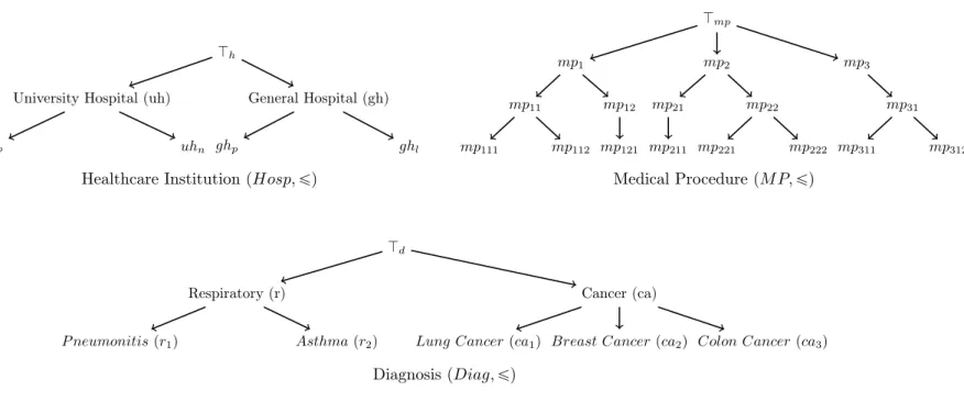
in form of taxonomies, classification or concept hierarchies. Each element in the hospitalization can be represented at different levels of granularity, by using a taxonomy (see Figure 1).
Our goal is to find specific patterns that appears frequently in patients trajectories’, by taking advantage of different levels of granularity for each element as background knowledge. Such patterns are very helpful to improve hospitalization planning, optimize clinical processes or detect anomalies.
2.2
Basic definitions
We assume in the following that domain knowledge always exists in the form of taxonomies. A sequence is an ordered set of vectors whose components are items or itemsets. Each item is a node
M ining H eter ogene ous M ultidimensional Se quential Patterns 5 ’ Jh
University Hospital (uh) General Hospital (gh) uhp uhn ghp ghl
Jmp
mp1 mp2 mp3
mp11 mp12 mp21 mp22 mp31
mp111 mp112 mp121 mp211 mp221 mp222 mp311 mp312
Healthcare InstitutionpHosp, ďq Medical ProcedurepM P, ďq
Jd
Respiratory (r) Cancer (ca)
P neumonitispr1q Asthmapr2q Lung Cancerpca1q Breast Cancer pca2q Colon Cancer pca3q
DiagnosispDiag, ďq
Figure 1: Taxonomies for the healthcare institution, the medical procedure and the diagnosis
RR
n
°
in a taxonomy. For the sake of simplicity we call a multidimensional sequence a“md-sequence" and we define it as follows:
Definition 1. (md-sequence)
A md-sequence s=xs1, s2, ..., sny is defined as set of elementary vectors si “ pe1, ..., ekq ordered
by the temporal order relation ăt such as s1 ăt s2 ăt s3... ătsn, where n is called the size of
the sequence s; i.e.,|s| “ n.
The vector e “ pe1, ..., ekq is more specific than e1 “ pe11, ..., e1kq, denoted by e ď e1, iff
eiď e1ifor all iď k. Then, ordering over md-sequence is defined as follows
Definition 2. (Ordering of Multidimensional Sequences) Given two md-sequences s “ xs1, s2, ..., sn1y and s
1 “ xs1
1, s12, ..., s1n2y, the sequence s “
xs1, s2, ..., sn1y is more specific than s
1 “ xs1
1, s12, ..., s1n2y, denoted by s ď s
1, if there exist a
set of indices 1ď i1ă i2ă ... ă in2 ď n1 such that sj ď s
1
ij for all jP t1 . . . n2u and n2ď n1.
s1 is said to be more general than s.
Example 1. Consider the three taxonomies pHosp, ďq, pDiag, ďq and pM P, ďq in Figure 1. The elementary vector e“ puhp, ca1,tmp111, mp121uq is more specific than e1 “ puh, ca, tmp11,
mp12uq, as uhp ď uh, ca1 ď ca and tmp111, mp121u ď tmp11, mp12u. The sequence s “
xpuhp, ca1,tmp111, mp121uq, pghl, r2,tmp121, mp131uqy is a md-sequence with two elementary
vec-tors s1 “ puhp, ca1,tmp111, mp121uq and s2 “ pghl, r2, tmp121, mp131uq where s1 comes before
s2 over time. The sequence s1“ xpuh, ca1,tmp11, mp12uq, pghl, r, tmp13uqy is more general than
s, as s1ď s11, s2ď s12 and s1 and s11 come before s2 and s12 over time.
Given a set MSDB “ ts1, s2, ..., smu of m md-sequences. The set MSDB is called a
mds-database. The support of an elementary vector in a mds-database is defined as follows: Definition 3. (Support of an elementary vector)
Let MSDBbe a mds-database and let e“ pe1, e2, ..., ekq be an elementary vector. The support
of the elementary vector e in MSDB, denoted by supppe, MSDBq, is defined as follows:
supppe, MSDBq “ |tsiP MSDB; Dj ď |si|; e ď siju|
While the support of a sequence s in MSDBis defined as follows:
Definition 4. (Support of md-sequence)
Let MSDB be a mds-database and let s be a md-sequence. The support of s, denoted by
suppps, MSDBq is defined as follows:
suppps, MSDBq “ |tsiP MSDB; siď su|
Given a positive integer σ as minimal support threshold, and a mds-database MSDB, the
elementary vector e is called frequent, iff supppe, MSDBq ě σ. A md-sequence is frequent in
MSDB if its support in MSDB exceeds the minimal support threshold σ. A frequent md-sequence is called a “mds-pattern". The problem of mining md-sequences is to enumerate all possible mds-patterns, given a mds-database MSDB and a minimal support threshold.
Example 2. The sequence s“ xpuh, ca, tmp11, mp2uq, pJh,Jd,tmp222uqy has a support which is
equal to 3 (i.e., suppps, MSDBq “ 3) in the database MSDB (see Table 1) and is a mds-pattern
Mining Heterogeneous Multidimensional Sequential Patterns 7
2.3
Most specific multidimensional sequential patterns
In this section, we present the problem of mining the most specific mds-patterns. Mining all possible mds-patterns from MSDB results in a huge amount of patterns that is difficult to
manage. Thus, we extract a set of mds-patterns that are not only frequent but also the most specific. This second constraint allows the reduction of the number of returned sequences by discarding patterns that are“too general". The most specific mds-pattern is defined as follows: Definition 5. (Most specific mds-pattern)
Given a positive integer σ as minimal support threshold and a mds-database MSDB. The
sequence s is a most specific mds-pattern in MSDBif and only if suppps, MSDBq ě σ and there
does not exist any sequence s1 such that suppps1, MS
DBq ě σ and s1ď s.
In this precise setting, the frequency for sequences ismonotone; i.e., whenever s is frequent, any generalization of s is also frequent. For example, if s “ xpuhp, ca1,tmp111, mp112uqy is
frequent in MSDB then s1 “ xpuh, ca, tmp1uqy which is more general than s is also frequent.
Thus, the most specific sequential patterns constitute a basic for retrieving all sequential patterns. Let σ“ 3 be a minimal support threshold, the sequence s “ xpuh, Jd,tmp1uq, pJh,Jd,tmp2uqy
is frequent, but is not the most specific one as the sequence s1 “ xpuh, ca, tmp
11, mp2uq, pgh, r,
tmp22, mp31uqy is frequent and verifies that s1ď s. The sequence s1is a most specific mds-pattern
as it is frequent and there is no other sequence in MSDB which is frequent and more specific.
The problem of mining mds-patterns is reduced to discover only the most specific patterns to significantly decrease the complexity of the problem and save computational time.
3
MMISP algorithm
In this section, we present an approach for extracting the most specific patterns from a mds-database MSDB. Our approach is called MMISP (Mining Multidimensional Itemsets
Sequential Patterns). The basic idea of MMISP consists in transforming the mds-data into a “classical form” (i.e., sequence of itemsets) and then applying a standard algorithm for sequential pattern mining. MMISP is based on three steps:
1. Extraction of frequent elementary vectors
The algorithm searches for the frequent and specific elementary vectors. 2. Transformation
In this step, all frequent elementary vectors are mapped into an alternate representation, then, the mds-database is encoded by using this new representation.
3. mds-patterns mining
In this step, a standard sequential algorithm is applied to the sequential database produced at the preceding step.
3.1
Step 1: Extracting all frequent elementary vectors:
The basic step in MMISP is extracting all frequent elementary vectors from MSDB w.r.t. the
ordering relation existing between their elements.
If the elementary vector is infrequent, then neither it nor its specifications will appear in mds-patterns. Thus, MMISP extracts only the frequent elementary vectors from MSDBto find
all the most specific mds-patterns. The main challenge in this step ishow to efficiently mine the frequent elementary vectors.
Assume that we have an elementary vector, composed of k bottom elements (i.e., K“ pK1
, ...,Kkq), is more specific than any other elementary vector. If element of the vector is an
item, then we consider a nodeKiconnected by edges to all leaves of taxonomy as a bottom node.
Otherwise if the element is an itemset, then the bottom is a set of all the leaf nodes. In our running example, the bottom elementary vector is pKh,Kd,tmp111, mp112, mp121, mp211, mp221, mp222,
mp311, mp312uq. The set of all the elementary vectors E with the bottom vector K is a lattice
pE Y tKu, ďq. Given two elementary vectors e “ pe1, ..., ekq and e1 “ pe11, ..., e1kq in E, the join
(\) of e and e1is defined as the join of ithelement in e and e1; i.e., e\ e1“ pe
1\ e11, ..., ek\ e1kq.
The join of two nodes in a taxonomy is the lowest common ancestor of these nodes, while the join of two set of nodes c“ tc1, ..., cnu and c1 “ tc11, ..., c1mu is the most specific values from the
sett@pi, jq; ci\ c1ju ; i ď n and j ď m.
Example 3. Consider the three taxonomiespHosp, ďq, pDiag, ďq and pM P, ďq in Figure 1, the two elementary vectors e“ puhp, ca2,tmp111, mp2uq and e1“ puhn, ca,tmp121, mp21uq. The join
of e and e1, e\ e1, is puh
p\ uhn, ca2\ ca, tmp111, mp2u \ tmp121, mp21uq, where the join of
uhp and uhn is uh , ca2 and ca is ca and the join oftmp111, mp2u and tmp121, mp21u is the set
tmp1, mp2u. Thus, the The join of e and e1 is the elementary vector puh, ca, tmp1, mp2uq.
The meet ([) of two elementary vector e and e1 is e[ e1 “ pe1[ e1
1, ..., ek[ e1kq. The meet
between two nodes in a taxonomy is the most specific one if they are comparable, otherwise it is the bottom nodeKi. The meet of two set of nodes c“ tc1, ..., cnu and c1“ tc11, ..., c1mu is the
most specific values from the set of the ancestors of each item in the two sets c and c1.
Example 4. Consider the three taxonomies pHosp, ďq, pDiag, ďq and pM P, ďq in Figure 1, the two elementary vectors e“ puhp, ca2,tmp111, mp2uq and e1“ puhn, ca,tmp121, mp21uq. The
meet of e and e1, e[ e1, ispuh
p[ uhn, ca2[ ca, tmp111, mp2u [ tmp121, mp21uq, where the meet
of uhp and uhn is Kh , ca2 and ca is ca2 and the meet of tmp111, mp2u and tmp121, mp21u
is the set tmp111, mp121, mp21u. Thus, the The meet of e and e1 is the elementary vector pKh
, ca2,tmp111, mp121, mp21uq.
Finally, we can say that pE Y tKu, ďq is a lattice, while the frequent elementary vectors considers as a join-semilattice pF E, ďq. The main challenge now is how to efficiently build the join-semilattice pF E, ďq. This task is achieved through a depth-first, and from left-to-right traversal [15], starting from the most general elementary vector J “ pJ1, ...,Jkq, we consider
it as frequent elementary vector. Then, for each frequent elementary vector e, we recursively generate all the immediate successors of e, and for each of them, we compute its support in MSDBand we keep the frequent one.
We need to define an effective and nonredundant way to characterize the immediate successors in pF E, ďq of a given elementary vector e “ pe1, ..., ekq as follows. Firstly, we will assume that
elements of the elementary vector are ordered according to a fixed total ordering. We will define an index z over the elementary vector to generate its immediate successors without redundancy and to buildpF E, ďq from left to right. This index is defined as the position of the element in ewhich is more specific thanJiand all the elements after this one until end of e are Ji (in the
case of e ispJ1, ...,Jkq, the index z equals to 1).
Example 5. Given the elementary vector e“ pJh, ca,Jmpq, then the index z equals to 2 as the
second element is notJd; i.e., e2“ ca, and all the elements after ca until end of e are top; i.e.,
e3“ Jmp.
To generate the immediate successors of an elementary vector e, we substitute each element in e, which has its position greater than or equal to the index z, with one of its immediate successors and the rest of the elements are kept as it is.
Mining Heterogeneous Multidimensional Sequential Patterns 9
puh, Jd,Jmpq pgh, Jd,Jmpq pJh, ca,Jmpq
puh, ca, Jmpq pgh, ca, Jmpq
pJh, ca1,Jmpq pJh, ca2,Jmpq pJh, ca3,Jmpq pJh, ca,tmp1uq pJh, ca,tmp2uq pJh, ca,tmp3uq Generated bypJh, ca,Jmpq Generated by puh, Jd,Jmpq Generated by pgh, Jd,Jmpq
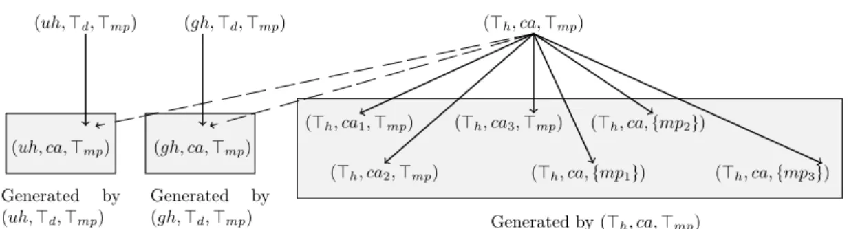
Figure 2: The immediate successors ofpJh, ca,Jmpq
Example 6. Given the same previous example e“ pJh, ca,Jmpq, as we see that the index z in
e is equal to 2, then its immediate successors are consisted of two sets. The first one contains all the elementary vectors which are generated by substituting the second element ca with one of its immediate successors and keeping the first and the third element; i.e.,Jh andJmp respectively.
While the second set contains all the elementary vectors which are generated by substituting the third element Jmp with one of its immediate successors and keeping the first and the second
element; i.e., Jh and ca respectively.
The immediate successors of an element depend on its type, if an element is an item then we follow the standard definition of immediate successor in the taxonomy. For example, given the taxonomypDiag, ďq in Figure 1, the immediate successors of ca are ca1, ca2and ca3.
In case, the element is an itemset c“ tc1, c2, ..., cmu, then to generate nonredundant
immedi-ate successors of c, we assume that its items are ordered according to a fixed total ordering. The immediate successors of c are splitted into two sets. The first one is generated by substituting the last item in c; i.e., cm, with one of its immediate successors and the rest of the items are kept
as it is; i.e., the first set of the immediate successors of c contains an itemset c1 “ tc1
1, ..., c1mu
where c1
i “ ci for all iă m and c1mis one of the immediate successors of cm. The second set is
generated by adding new item cm`1to end of c, where cm`1is one of the right siblings of cmand
all its ancestor nodes; i.e., the second set of the immediate successors of c contains an itemset c1“ tc1
1, ..., c1m, c1m`1u where ci1 “ ci for all iď m and c1m`1is one of the right siblings of cmand
all its ancestor nodes.
Example 7. Given the taxonomy pM P, ďq in Figure 1, the immediate successors of c “ tmp1,
mp21u are generated by substituting the last item mp21 in c with its immediate successors; i.e.,
tmp1, mp211u, and by adding the right siblings of mp21 and all its ancestor nodes; i.e., mp22 and
mp3, to the end of c; i.e.,tmp1, mp21, mp22u and tmp1, mp21, mp3u.
Given the taxonomies in Figure 1, the immediate successors of e “ pJh, ca, Jmpq are
puh, ca, Jmpq, pgh, ca, Jmpq, pJh, ca1,Jmpq, pJh, ca2,Jmpq, pJh, ca3,Jmpq, pJh, ca,tmp1uq, pJh,
ca,tmp2uq and pJh, ca,tmp3uq. The first two are generated from puh, ca, Jmpq and pgh, ca, Jmpq
respectively, while the rest are generated from pJh, ca, Jmpq. First by replacing only ca with
one of ca1, ca2 and ca3 and keeping Jh and Jmp; i.e., pJh, ca1,Jmpq, pJh, ca2,Jmpq and
pJh, ca3,Jmpq. Then, by replacing only Jmpwith one oftmp1u, tmp2u and tmp3u and keeping
Jh and ca; i.e.,pJh, ca,tmp1uq, pJh, ca,tmp2uq and pJh, ca,tmp3uq (see Figure 2).
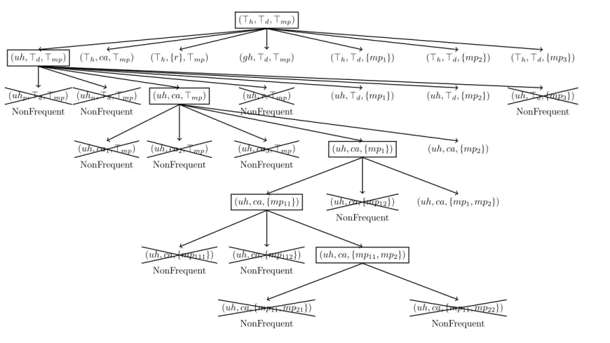
The frequency of an elementary vector is monotone, the specialization of a non-frequent ele-mentary vector is also non-frequent. We use this monotonicity to prune the enumeration space and efficiently build the semilatticepF E, ďq. Figure 3 shows an example of generation of a part
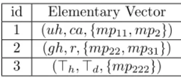
id Elementary Vector 1 puh, ca, tmp11, mp2uq
2 pgh, r, tmp22, mp31uq
3 pJh,Jd,tmp222uq
Table 2: The most specific frequent elementary vectors extracted frompF E, ďq.
of pF E, ďq with σ “ 3 which is detailed as follows. As the first step we consider the most general elementary vector pJh,Jd,Jmpq, from which seven new frequent elementary vectors,
puh, Jd,Jmpq, pgh, Jd,Jmpq, pJh, r,Jmpq, pJh, ca,Jmpq, pJh,Jd,tmp1uq, pJh,Jd, tmp2uq and
pJh,Jd,tmp3uq, are generated. Let us consider the first elementary vector, puh, Jd,Jmpq, the
im-mediate successors generate byMMISP arepuh, ca, Jmpq, puh, Jd,tmp1uq and puh, Jd,tmp2uq.
Now, for the vector puh, ca, Jmpq obtained in the previous level, further immediate successors
puh, ca, tmp1uq and puh, ca, tmp2uq are generated. Similarly we obtain the following two vectors
puh, ca, tmp11uq and puh, ca, tmp1, mp2uq and puh, ca, tmp11, mp2uq from puh, ca, tmp1uq and
puh, ca, tmp11uq respectively. Finally, for the vector puh, ca, tmp11, mp2uq, no any new frequent
elementary vectors can be found, thus the generation stops.
As the objective ofMMISP is extracting the most specific sequential patterns, we retain only the most specific elementary vectorsMSFEV inpF E, ďq. The most specific frequent elementary vectors constitute collection of elementary vectors in MSDBwith respect to σ which are frequent
and most specific. Table 2 shows the set of most specific frequent elementary vectors which are extracted frompF E, ďq.
The pseudocode of the first step inMMISP is presented in Algorithm 1. The idea is simple: Lines 2-3 generate the most general elementary vector e“ pJ1, ...,Jmq, while Line 6 adds e to
pF E, ďq. Then, Line 7 recursively calls the function get_rec_msf ev starting from e to build the join-semilattice pF E, ďq and to get all the most specific frequent elementary vectors M SF EV .
Algorithm 2 presents the pseudocode of the function get_rec_msf ev. Lines 2-5 get the index zin e, Line 6 generates the immediate successor of e based on the index z, while Line 7 keeps only the frequent ones. When there are no frequent immediate successors of e, then e considers as one of the most specific frequent elementary vectors (see Lines 8-9). Otherwise, we call recursively the function get_rec_msf ev for each frequent immediate successors of e (Lines 10-13).
Algorithm 3 shows how to generate immediate successors of an elementary vector. Line 2 shows that generation starts from the zthelement. Lines 3-9 show that if an element is an item,
we substitute it with one of its immediate successors and the rest of the elements are kept as it is. While, if an element is an itemset c, we substitute it with another itemset. This itemset is generated by substituting the last item in c with one of its immediate successors (Lines 13-17). Then, by appending the right sibling of last item in c at its end (Lines 18-22). Finally, by appending the right siblings of all the ancestors of last item in c at its end (Lines 23-29).
3.2
Step 2: Transformation of mds-database:
We now study the temporal relation between the extracted specific frequent elementary vectors as follow. Firstly, we replace each elementary vector in each md-sequence of MSDB with all its
generalizations from MSFEV set. Given a sequence s“ xs1, ..., sny in MSDB the replacement
consists in substituting each elementary vector si in s by several elementary vectors eP MSFEV
such that siď e.
M ining H eter ogene ous M ultidimensional Se quential Patterns 11 pJh,Jd,Jmpq
puh, Jd,Jmpq pJh, ca,Jmpq pJh,tru, Jmpq pgh, Jd,Jmpq pJh,Jd,tmp1uq pJh,Jd,tmp2uq pJh,Jd,tmp3uq
puhp,Jd,Jmpq
NonFrequent
puhn,Jd,Jmpq
NonFrequent
puh, ca, Jmpq puh, r, Jmpq
NonFrequent
puh, Jd,tmp1uq puh, Jd,tmp2uq puh, Jd,tmp3uq
NonFrequent puh, ca1,Jmpq NonFrequent puh, ca2,Jmpq NonFrequent puh, ca3,Jmpq NonFrequent
puh, ca, tmp1uq puh, ca, tmp2uq
puh, ca, tmp11uq puh, ca, tmp12uq
NonFrequent puh, ca, tmp1, mp2uq puh, ca, tmp111uq NonFrequent puh, ca, tmp112uq NonFrequent puh, ca, tmp11, mp2uq puh, ca, tmp11, mp21uq NonFrequent puh, ca, tmp11, mp22uq NonFrequent
Figure 3: The steps of generating the elementary vectors in pF E, ďq with σ “ 3.
RR
n
°
Algorithm 1:Mining All The Most Specific Frequent Elementary Vector
input : mds-database MSDB, Minimum support threshold σ, Set of m taxonomies
T ax“ tT ax1, ..., T axmu.
output: The set MSFEV of all most specific frequent elementary vectors, The join semi-lattice FE.
begin
/* Generating the most general elementary vectors pJ1,J2, ...,Jmq */
foriÐ 1 to m do ei=Ji;
M SF EV Ð H ; F E Ð H ;
F E Ð F E Yt e u ;
/* The recursive method to build the join-semilattice pF E, ďq and to get all the most specific frequent elementary vectors M SF EV . */ call get_rec_msf ev(MSDB,e,σ,Tax,F E,M SF EV );
Algorithm 2:Routine get_rec_msf ev
input : mds-database MSDB, Elementary vector e, Minimum support threshold σ, Set of
mtaxonomies T ax“ tT ax1, ..., T axmu, Set of frequent elementary vectors F E,
Set of most specific elementary vectors M SF EV . begin
/* Computing the index z */
z =1;
foriÐ 1 to m do if ei‰ Ji then
z =i;
Cand Ð immediate_successor_elementary_vector(e,z,T ax) ; F req Ð t e1 P Cand ; supppe1, MS
DBq ě σu;
if F req = H then
/* e is a most specific elementary vector */ M SF EV Ð M SF EV Yt e u ;
else
/* Recursive call get_rec_msf ev for each new frequent elementary
vector generated */
foreache1 P F req do
F E Ð F E Yt e1 u ;
Mining Heterogeneous Multidimensional Sequential Patterns 13
Algorithm 3: Routine immediate_successor_elementary_vector
input : Elementary vector e, Index z, Set of m taxonomies T ax“ tT ax1, ..., T axmu.
output: A set of immediate successors of e. begin
foriÐ z to m do
/* In cas the element ei is an item */
if ei is an item then foreachx P immediate_successor (ei,T axi) do e1 =e; e1i=x ; OutputÐ Output Y t e1 u ; end end
/* In cas the element ei is an itemset */
else if ei is an itemset then
c“ ei;
k“ |c| ;
/* Replacing the last item in c with its immediate successor */ foreachx1 P immediate_successor (c k,T axi) do e1 =e; e1i“ append_at_endpczck, x1q ; OutputÐ Output Y t e1 u ; end
/* Appending the right sibling of ck at the end of c */
foreachx1P right_siblingpc k, T axi) do e1 =e; e1 i“ append_at_endpc, x1q ; OutputÐ Output Y t e1 u ; end
/* Appending the right sibling of all the ancestors of ck at the
end of c */ foreachxP ancestorspck, T axi) do foreachx1P right_siblingpx, T ax i) do e1 =e; e1i“ append_at_endpc, x1q ; OutputÐ Output Y t e1 u ; end end end return Output ; end RR n° 8521
Patients Trajectories p
s1 xtpuh, ca, tmp11, mp2uqu, tpJh,Jd,tmp222uqu, tpgh, r, tmp22, mp31uquy
p
s2 xtpuh, ca, tmp11, mp2uqu, tpJh,Jd,tmp222uq, pgh, r, tmp22, mp31uquy
p
s3 xtpuh, ca, tmp11, mp2uqu, tpJh,Jd,tmp222uq, pgh, r, tmp22, mp31uquy
p
s4 xtpuh, ca, tmp11, mp2uq, pJh,Jd,tmp222uqu, tpgh, r, tmp22, mp31uqu, tpgh, r, tmp22, mp31uquy
Table 3: A mds-database yMSDB which is the transformation of the patient trajectories in
Table 1 by using the set of all most specific frequent elementary vector in Table 2. Patients Trajectories
p
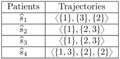
s1 xt1u, t3u, t2uy
p
s2 xt1u, t2, 3uy
p
s3 xt1u, t2, 3uy
p
s4 xt1, 3u, t2u, t2uy
Table 4: Transformed database in Table 3
intoxtpuh, ca, tmp11, mp2uq, pJh,Jd,tmp222uqu, tpgh, r, tmp22, mp31uqu, tpgh, r, tmp22, mp31uquy
where:
• The elementary vector s41,puhp, ca2,tmp112, mp222uq, is replaced by puh, ca, tmp11, mp2uq and
pJh,Jd,tmp222uq from MSFEV set in Table 2, with s41ď puh, ca, tmp11, mp2uq and s41ď pJh,
Jd,tmp222uq.
• The elementary vector s42and s43,pghp, r2,tmp221, mp312uq, are replaced by pgh, r, tmp22, mp31uq
from MSFEV set.
Table 3 shows the transformation of MSDB in Table 1 based on the set of all most specific
frequent elementary vectorsMSFEV in Table 2. Transformation of MSDBdenoted by yMSDB.
3.3
Step 3: mds-patterns mining:
In a classical sequential pattern mining algorithm, the sequential database to be mined should be represented as a set of pairspsid, sq where sid is a unique sequence identifier and s is a sequence of itemsets. To apply this algorithms on yMSDB, we transformed it as follows:
• Each elementary vector inMSFEV is assigned a unique id which is used during the mining (see Table 2).
• For each sequence psi in yMSDB and for each elementary vector e inpsij wherepsij Ppsi, e is
replaced by its id.
Example 9. The sequenceps4“ xtpuh, ca, tmp11, mp2uq, pJh,Jd,tmp222uqu, tpgh, r, tmp22, mp31uqu,
tpgh, r, tmp22, mp31uquy in yMSDB(see Table 3) is transformed intoxt1, 3u, t2u, t2uy as: ptuhu, tcau,
tmp11, mp2uq, ptghu, tru, tmp22, mp31uq and pJh,Jd,tmp222uq inps4has id 1, 2 and 3 respectively
in Table 2.
Table 4 shows the transformation of the database yMSDB in Table 3 by using the identifiers
Mining Heterogeneous Multidimensional Sequential Patterns 15
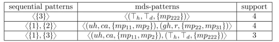
sequential patterns mds-patterns support xt3uy xpJh,Jd,tmp222uqy 4
xt1u, t2uy xpuh, ca, tmp11, mp2uq, pgh, r, tmp22, mp31uqy 4
xt1u, t3uy xpuh, ca, tmp11, mp2uq, pJh,Jd,tmp222uqy 3
Table 5: All the most specific sequential patterns extracted from MSDBin Table 1 with σ“ 3.
We use CloSpan [8] as a sequential pattern mining algorithm to extract sequential patterns form Table 4. Table 5 displays all sequential patterns in their transformed format and the frequent patient trajectories in which identifiers are replaced with their actual values, with σ“ 3.
These 3 steps allow us to extract from heterogeneous multidimensional sequential database patterns that include elements with different levels of granularity.
4
Implementation and Experimental Validation
We conduct experiments on both real and synthetic datasets. The MMISP algorithm is imple-mented in Java and the experiments are carried out on a MacBook Pro with a 2.5GHz Intel Core i5, 4GB of RAM Memory running OS X 10.6.8. Extraction of sequential patterns is based on the public implementation of CloSpan algorithm [8] supplied by the IlliMine1 toolkit.
4.1
Healthcare Trajectory
4.1.1 Mining healthcare trajectories
In order to assess the effectiveness of our approach, we run several experiments on PMSI2, which
is a French national information system for managing hospital activity with both economical and medical points of view. This section describes the results obtained after applying MMISP on a set of 2600 patients suffering from lung cancer who live in the Lorraine region, of Eastern France. We reconstituted the sequence of hospitalizations of patients who have treatment between 2006 and 2010. Each event in a sequence was characterized by the following dimensions : hospital, principal diagnosis, medical procedures delivered during the stay.
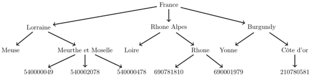
Thehospital dimension was associated with a geographical taxonomy of 4 levels, first level refers to the root (France) and second, third and fourth level correspond to administrative region, administrative department and hospital respectively. Figure 4 illustrates University Hospital of Nancy (code: 540002078) as a hospital in Meurthe et Moselle, which is a department in Lorrain in the Region of France. There are 151 nodes in this taxonomy.
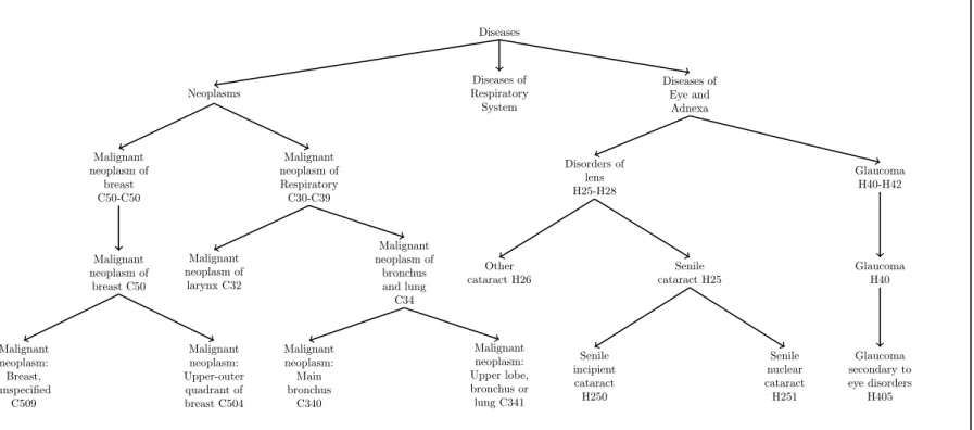
The principal diagnosis dimension could be described at 5 levels of the 10th International
classification of Diseases (ICD10): root , chapter, block, 3-character, 4-character, terminal nodes. Figure 5 depicts chapters such as N eoplasms have specializations: block C30´C39 is a malignant neoplasms of respiratory, block C50´ C50 which is a malignant neoplasms of breast etc. The block C30´ C39 has specializations: malignant neoplasm of larynx (code: C34), malignant neoplasm of bronchus and lung (code: C32), etc. C34 (Lung cancer) has specializations: C340 is a cancer of the main bronchus, C341 is a cancer of upper lobe etc. The number of nodes in the disease taxonomy is 990 nodes.
1
http://illimine.cs.uiuc.edu/ 2
Programme de Médicalisation des Sytèmes d’Information.
France
Lorraine Rhone Alpes Burgundy
Meuse Meurthe et Moselle Loire Rhone Yonne Côte d’or 540000049 540002078 540000478 690781810 690001979 210780581
Figure 4: A geographical poset of the healthcare institution
Patients Trajectories
P atient1 xp540002078, C341, tZBQKuq, p570023630, Z51, tZBQK, GF F Auq, . . .y
P atient2 xp100000017, C770, tZBQKuq, p210780581, C770, tZZQK, Y Y Y Y uq, . . .y
P atient3 xp210780110, H259, tY Y Y Y uq, p210780110, H259, tZZQKuq, . . .y
Table 6: Care trajectories of 3 patients
Themedical procedures dimension can have 5 levels of CCAM3which is a French nomenclature
for coding procedures performed by physicians. For example, ZBQK is a chest radiography for respiratory system, which is one of the procedures applied for respiratory diseases. These procedures are a part of the respiratory procedure which in turn is included in the medical procedure.
Table 6 shows an example of care trajectories for 3 patients. For example, P atient1 has two
hospitalizations, the first was in the University Hospital of Nancy (code: 540002078) for lung cancer (code: C341) where he underwent a chest radiography (code: ZBQK). Then, he was hospitalized in a private clinic in Metz (code: 570023630), for a chemotherapy session (code: Z51) where he had a chest radiography and pneumonectomy (code: GF F A).
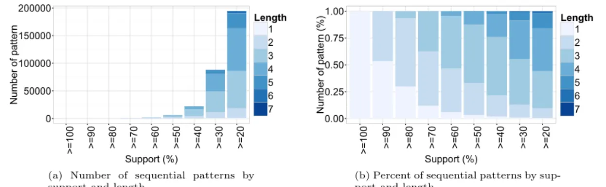
In this experiment, the support value is set to 500 patients (i.e. σ“ 20%). MMISP generates 194 650 different frequent trajectories. Figure 6.a shows the number of discovered patterns at different thresholds according to their length. With support threshold equals 20%, the high num-ber of length 3 and 4 patterns is explained by a combinatorial effect resulting from a high numnum-ber of sequences of length 5-11 in the database. These frequent sequences correspond to the patients who underwent chemotherapy and usually had around 3 and 6 stays for 1 cycle. Figure 6.b shows the percentage discovered patterns at different thresholds according to their length. Here we can observe that 80% of patterns for which support is over 20% have at most 4 hospitalizations which correspond to the case where in each hospitalization the patient underwent chemotherapy. With support threshold equals to 100%, there is only one pattern xpF rance, C34,tZBQKuqy
which shows that 100% of the patients in France whose had a Lung cancer they underwent chemotherapy during their visit.
Table 7 shows the items appearing in principal diagnosis dimension of patterns for which support is over 40%. It can be noticed that the ICD10 tree has been mined at different levels. In the neoplasm branch, the most specific observed item is of depth 3, “ malignant neoplasm of bronchus and lung”. In the branch of “factors influencing health status and contact with health services”, items of depth 4 (“chemotherapy session for neoplasm") have been extracted. Children of“Malignant neoplasm of bronchus and lung” are not frequent enough to be extracted, but “chemotherapy session” appears in a sufficient proportion of trajectories to be seen. Such results cannot be obtained by representing items at an arbitrary pre-determined level.
3
M ining H eter ogene ous M ultidimensional Se quential Patterns 17 Diseases Neoplasms Diseases of Respiratory System Diseases of Eye and Adnexa Malignant neoplasm of breast C50-C50 Malignant neoplasm of Respiratory C30-C39 Disorders of lens H25-H28 Glaucoma H40-H42 Malignant neoplasm of breast C50 Malignant neoplasm of larynx C32 Malignant neoplasm of bronchus and lung C34 Other cataract H26 Senile cataract H25 Glaucoma H40 Malignant neoplasm: Breast, unspecified C509 Malignant neoplasm: Upper-outer quadrant of breast C504 Malignant neoplasm: Main bronchus C340 Malignant neoplasm: Upper lobe, bronchus or lung C341 Senile incipient cataract H250 Senile nuclear cataract H251 Glaucoma secondary to eye disorders H405
Figure 5: A disease taxonomy
RR
n
°
0 50000 100000 150000 200000 >=1 0 0 >=9 0 >=8 0 >=7 0 >=6 0 >=5 0 >=4 0 >=3 0 >=2 0 Support (%) N u mb e r o f p a tt e rn Length 1 2 3 4 5 6 7 0.00 0.25 0.50 0.75 1.00 >=1 0 0 >=9 0 >=8 0 >=7 0 >=6 0 >=5 0 >=4 0 >=3 0 >=2 0 Support (%) N u mb e r o f p a tt e rn (% ) Length 1 2 3 4 5 6 7
(a) Number of sequential patterns by support and length.
(b) Percent of sequential patterns by sup-port and length.
Figure 6: Distribution of sequential patterns by support and length ICD10 level – Diagnosis Taxonomy
0– Root 1– Neoplasms
2– Malignant neoplasms of respiratory and intrathoracic organs (C30–C39) 3– Malignant neoplasm of bronchus and lung (C34)
1– Factors influencing health status and contact with health services
2– Persons encountering health services for specific procedures and health care (Z40-Z54) 3– Other medical care (Z51)
4– Chemotherapy session for neoplasm (Z511)
Table 7: Items extracted in the Principal Diagnosis dimension, (minimal support equals to 40%)
The mds-patterns can be analyzed per se. For example, the patternxpLorraine, C34, tChemo, P neumouqy shows that 93% of patients had pneumonectomy and chemotherapy for a lung cancer in any hospital in Lorraine Region in France. The pattern xpLorraine, TDiag,tZ40 ´
Z54uq, pLorraine, C34, tChemo, P neumuq, pLorraine, TDiag, tZ51uqy shows that 59% of
pa-tients had three hospitalizations where in the first one they started their treatment by under-doing chemotherapy then having pneumonectomy and chemotherapy for a lung cancer and a subsequent stay in the Lorraine Region for complementary treatments and follow-up.
This kind of information helps healthcare managers and deciders in planning and organizing healthcare resources at a regional level. Besides, sequential patterns can be seen as a condensed representation of care trajectories. As such, patterns can be reused as new variables to distinguish subgroups of patients in subsequent analysis.
4.1.2 MMISP versus Standard sequential pattern mining method
In this section, we compareMMISP with a standard sequential pattern mining method such as CloSpan [8]. All standard sequential pattern mining algorithms require that the dataset to be mined is composed of pairs of the formpid, seqq, where id is a sequence identifier and seq is a sequence of itemsets. We transfer each sequence siin MSDB with anextended-sequencepsi. Each
elementary vector of a sequence si is transformed into a single itemset by replacing its elements
with all its ancestors. For example, the elementary vector (uhp, ca1,tmp111, mp221u) would be
replaced with tJh, uh, uhp, Jd, ca, ca1, Jmp, mp1, mp2, mp11, mp22, mp111, mp221u as
uhhď uh ď Jh, ca1ď ca ď Jd, mp111ď mp11ď mp1ď Jmpand mp221ď mp22ď mp2ď Jmp.
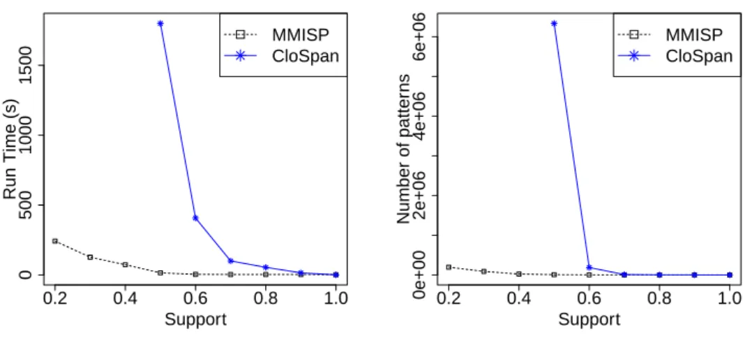
Mining Heterogeneous Multidimensional Sequential Patterns 19 0.2 0.4 0.6 0.8 1.0 0 500 1000 1500 Support MMISP CloSpan Run Time (s)
(a) Runtime sequences over frequency threshold
0.2 0.4 0.6 0.8 1.0 0e+00 2e+06 4e+06 6e+06 Support MMISP CloSpan Number of patter ns
(b) Number patterns over frequency threshold
Figure 7: MMISP versus CloSpan
database. This way of managing hierarchies has been used in GSP which is proposed by [5]. Our main goal is to evaluate the quality of the frequent trajectories mined withMMISP and its performance compared to naive approach usingCloSpan. We firstly transform the 2400 patients trajectories, then we apply the two approaches using minimum supports threshold ranging from 100% to 20%. Figure 7 reports the execution time and the number of frequent trajectories according to different values of support threshold for bothCloSpan and MMISP.
Actually,CloSpan cannot finish its calculations for support threshold less than 50% because the transformation increases number of items in itemset and generates a large number of density similar sequences. Whereas,MMISP runs in acceptable time for support as low as 20%.
MMISP is able to extract condensed frequent trajectories w.r.t. the ones mined by CloSpan. For example, the trajectoryxtJh, uh,Jd, ca,Jmp, mp1, mp2, mp11u tJh, gh,Jd, r,Jmp, mp2, mp3,
mp22, mp31uy generated by CloSpan contains redundant information as a hospitalization
con-taining mp22will also containJmp and mp2. MMISP is not affected by this pattern because it
extracts just the most specific frequent elementary vector in the first step of the algorithm. CloSpan extracts all the frequent trajectories (i.e., the general and specific ones) while MMISP generates just the more specific ones. For example, ifxpJh,Jd,tmp222uqy is a frequent trajectory.
MMISP does not extract the trajectories which are more general like xpJh,Jd,tmp22uqy while
CloSpan extracts both the general and specific ones. Figure 7 shows the difference between the number of frequent trajectories extracted byCloSpan and MMISP. For example, with a support threshold of 70 %, MMISP extracts 565 frequent trajectories while CloSpan extracts 6 335 683 frequent trajectories.
Finally, we may conclude that:
• MMISP is more efficient than CloSpan over extended-sequential database with low support threshold.
• The trajectories extracted by CloSpan require post processing while this is not the case withMMISP.
• MMISP extracts just the most specific frequent trajectories while CloSpan extracts both general and specific ones. This means that CloSpan extracts a huge number of patterns. Analyzing all of them is not an easy task for healthcare managers and decision makers.
4.1.3 M M ISP versus M3
SP
Another experiment is carried out for comparing M3
SP with MMISP. Our main goal is to evaluate the effectiveness of sequential patterns mined byMMISP compared to the ones extracted by M3
SP. For this purpose, we applied M3
SP with hospital, diagnosis and medical procedures as analysis dimensions. The support value is set to 500 patients (i.e. σ“ 20%). Table 8 reports an example of the extracted patterns with M3
SP andMMISP.
Firstly, we observe thatMMISP is able to extract condensed trajectories w.r.t. the ones mined by M3
SP. For example, 48 trajectories, Pattern #1,..., Pattern #48, generated by M3
SP are summarized by3 ones, Pattern #50, Pattern #51 and Pattern #52, extracted by MMISP (see Table 8). This shows that the rigid structure of multidimensional item assumed by M3
SP limits the expressivity of the results.
Besides that, in M3
SP, several dimensions can be repeated at the same hospitalization. For example, in M3
SP, Pattern #48 represents one hospitalization including 9 multidimensional items. Each multidimensional item is associated with the same value of hospital and diagnosis (540002078 and C341) and different values of medical procedures. In MMISP, Pattern #50 (extracted by MMISP ) represents the same trajectory as Pattern #48. Pattern #50 has one elementary vector with three elements: hospital 540002078, diagnosis C341 and a set of medical procedure tZBQK, DEQP, GF F A, GLLD, GELD, ZZQK, GELE, F CF A, AGLBu. Pattern #50 is much more compact and informative than Pattern #48.
Given a minsup threshold,MMISP extracts sequential patterns that are not found by M3
SP. For instance, Pattern #53 extracted by MMISP is not found by M3
SP. This is due to the fact thatMMISP extracts new frequent hospitalizations not extracted by M3
SP. For instance e=(Lorraine,JDiseases, {GEQE, ACQH, ZCQH}) and e1=(Lorraine,Diseases of the Respiratory,
{ACQH}) are extracted by MMISP. As e and e1 are frequent and not comparable (i.e. e ę e1
and e1 ę e), M3
SP extracts only (Lorraine, Diseases of the Respiratory, ACQH) and not (Lorraine,JDiseases, ACQH) as (Lorraine, Diseases of the respiratory, ACQH) is more specific
than(Lorraine,JDiseases, ACQH).
From a quantitative point of view,MMISP extracts 419 frequent hospitalizations with 194 650 frequent trajectories while M3
SP extracts102 multidimensional items with 1 242 frequent tra-jectories. The execution time of M3
SP is about 82 seconds while MMISP takes about 242 seconds.
Finally, we may conclude that:
• Several frequent trajectories generated by M3
SP can be summarized by only one mined byMMISP.
• Several multidimensional items generated by M3
SP can be summarized by only one ele-mentary vector inMMISP.
• One elementary vector inMMISP represents one hospitalization in the trajectory while one multidimensional item in M3
SP represents only a part of hospitalization in the trajectory. • Some frequent trajectories can be extracted by MMISP while they can not be extracted
by M3
Mining Heterogeneous Multidimensional Sequential Patterns 21
Methods id Trajectory Patterns M3
SP
1 xtp540002078, C341, GF F Aqp540002078, C341, ZZQKquy
2 xtp540002078, C341, DEQP qp540002078, C341, GF F Aqp540002078, C341, ZZQKquy . . . 48 xtp540002078, C341, ZBQKqp540002078, C341, DEQP qp540002078, C341, GF F Aq p540002078, C341, GLLDqp540002078, C341, GELDqp540002078, C341, ZZQKq p540002078, C341, GELEqp540002078, C341, F CF Aqp540002078, C341, , AGLBquy 49 xpLorraine, Diseases of the respiratory, ACQHqy
MMISP
50 xtp540002078, C341, tZBQK, DEQP, GF F A, GLLD, GELD, ZZQK, GELE, F CF A, AGLBuy 51 xp540002078, C341, tDEQP, GELD, GELE, ZZQK, AGLB, GLLD, GF F Auqy 52 xp540002078, C341, tZBQK, DEQP, GELD, GELE, ZZQK, GLLD, GF F Auqy 53 xpLorraine, JDiseases,tGEQE, ACQH, ZCQHuqy
Table 8: Some patterns obtained by M3
SP and MMISP.
4.2
Experiments on Synthetic Datasets
In this experiment, we study the scalability of the MMISP approach. We consider the number of extracted patterns and the running time with respect several parameters:
• number of elements in each elementary vector. • depth of the taxonomy of each component.
• number of elementary vectors in each sequence (i.e. sequence length). • number of sequences in a sequential database.
The first batch of synthetic data generated contains 1000 sequences defined over 2, 3, 4 and 5 elements in the elementary vector for each sequence. Each sequence contains 15 elementary vectors. Each taxonomy is defined over 3 levels of granularity between its items. Figure 8 reports the results according to different values of support threshold for different numbers of elements in the elementary vector. The running time increases for each newly added component.
In Figure 9, we study the performance ofMMISP by considering several levels of granularity for each taxonomy. We generated 1000 sequences defined over 15 elementary vectors. Each elementary vector has 3 components. Each taxonomy of the element is defined over 3, 4, 5, 6 levels of granularity. The number of extracted patterns does not change with each newly added level asMMISP extracts only the most specific sequential patterns. The execution time increases with the increase in the number of levels in a taxonomy because of the complexity of the product of taxonomies in the first step ofMMISP which generates all the frequent elementary vectors.
We study the performance ofMMISP and the number of extracted patterns with respect the number of sequences in a sequential database and the length of each sequence. Figure 10 shows the execution time and the number of patterns extracted for 1000 sequences with 3 dimensions associated with taxonomy with 3 levels of granularity and with varying sequence length. The execution time increases with the increase in length of a sequence. This is due to the third step ofMMISP which uses CloSpan to mine the transformed sequences.
Figure 11 shows the running time and the number of patterns extracted for several number of sequences (1000, 2000, 3000, 4000 and 5000 sequences) also with 3 dimensions associated with taxonomy with 3 levels of granularity. In these experiments, the sequence length is roughly 15.
Figures 8 - 11 highlight the fact that MMISP is efficient in terms of runtime for a large panel of sequences with varying different parameters.
0.10 0.12 0.14 0.16 0.18 0.20 200 400 600 800 Support ● ● ● ● ● ● ● 2 elements 3 elements 4 elements 5 elements Run Time (s)
(a) Runtime sequences over frequency threshold.
0.10 0.12 0.14 0.16 0.18 0.20 2000 4000 6000 8000 Support ● ● ● ● ● ● ● 2 elements 3 elements 4 elements 5 elements Number of P atter ns
(b) Number patterns over frequency threshold.
Figure 8: Number of sequential pattern extracted and Running time obtained byMMISP with varying in the length of elementary vectors.
0.10 0.12 0.14 0.16 0.18 0.20 0 500 1000 1500 Support ● ● ● ● ● ● ● 3 levels 4 levels 5 levels 6 levels Run Time (s)
(a) Runtime sequences over frequency threshold.
0.10 0.12 0.14 0.16 0.18 0.20 1000 3000 5000 7000 Support ● ● ● ● ● ● ● 3 levels 4 levels 5 levels 6 levels Number of P atter ns
(b) Number patterns over frequency threshold.
Figure 9: Number of extracted pattern (right) and Running Time (left) obtained by MMISP with varying over the levels of granularity between items of the taxonomies.
Mining Heterogeneous Multidimensional Sequential Patterns 23 0.10 0.12 0.14 0.16 0.18 0.20 0 500 1000 1500 2000 Support ● ● ● ● ● ● ● 10 vectors 15 vectors 20 vectors 25 vectors 30 vectors Run Time (s)
(a) Runtime sequences over frequency threshold.
0.10 0.12 0.14 0.16 0.18 0.20 2000 6000 10000 14000 Support ● ● ● ● ● ● ● 10 vectors 15 vectors 20 vectors 25 vectors 30 vectors Number of P atter ns
(b) Number patterns over frequency threshold.
Figure 10: Number of sequential pattern extracted and Running time for a large panel of sequences when varying over sequence length.
0.10 0.12 0.14 0.16 0.18 0.20 0 1000 2000 3000 4000 Support ● ● ● ● ● ● ● 1000 seq 2000 seq 3000 seq 4000 seq 5000 seq Run Time (s)
(a) Runtime sequences over frequency threshold.
0.10 0.12 0.14 0.16 0.18 0.20 0 10000 30000 Support ● ● ● ● ● ● ● 1000 seq 2000 seq 3000 seq 4000 seq 5000 seq Number of P atter ns
(b) Number patterns over frequency threshold.
Figure 11: Number of sequential pattern extracted and Running time for a large panel of sequences when varying over several number of sequences.
5
Conclusion
This report presents a new approach to extract sequential patterns from heterogeneous multi-dimensional sequential database. We provide formal definitions and propose a new algorithm MMISP to mine this kind of data. This method mined the database which are often represented as a sequence of vector of heterogeneous elements with different types (i.e, item and itemset) takes into account background knowledge lying in term taxonomies for each dimension. We con-duct experiments on both real-world and synthetic datasets. The method is applied on real-world data where the problem is to mine healthcare patients trajectories and gives potential interesting patterns for healthcare specialists. For future work, we are planning to use statistical significance tests to evaluate the sequential patterns extracted and choose the most significant ones. On the other hand, proposing a graphical interface to visualize and query the sequential patterns.
References
[1] R. Agrawal and R. Srikant, “Mining sequential patterns,” in Proceedings of the Eleventh International Conference on Data Engineering, ser. ICDE ’95. Washington, DC, USA: IEEE Computer Society, 1995, pp. 3–14. [Online]. Available: http: //dl.acm.org/citation.cfm?id=645480.655281
[2] C. Chothia and M. Gerstein, “Protein evolution. how far can sequences diverge?” Nature, vol. 6617, no. 385, pp. 579–581, 1997.
[3] Q. Yang and H. H. Zhang, “Web-log mining for predictive web caching,” IEEE Trans. on Knowl. and Data Eng., vol. 15, no. 4, pp. 1050–1053, Jul. 2003.
[4] J. Serrà, H. Kantz, X. Serra, and R. G. Andrzejak, “Predictability of music descriptor time series and its application to cover song detection,” IEEE Transactions on Audio, Speech & Language Processing, vol. 20, no. 2, pp. 514–525, 2012.
[5] R. Srikant and R. Agrawal, “Mining sequential patterns: Generalizations and performance improvements,” in Proceedings of the 5th International Conference on Extending Database Technology: Advances in Database Technology, ser. EDBT ’96. London, UK, UK: Springer-Verlag, 1996, pp. 3–17. [Online]. Available: http: //dl.acm.org/citation.cfm?id=645337.650382
[6] M. J. Zaki, “Spade: An efficient algorithm for mining frequent sequences,” Mach. Learn., vol. 42, no. 1-2, pp. 31–60, Jan. 2001. [Online]. Available: http://dx.doi.org/10.1023/A: 1007652502315
[7] J. Pei, J. Han, B. Mortazavi-Asl, J. Wang, H. Pinto, Q. Chen, U. Dayal, and M. Hsu, “Mining sequential patterns by pattern-growth: The prefixspan approach,” IEEE Trans. Knowl. Data Eng., vol. 16, no. 11, pp. 1424–1440, 2004.
[8] X. Yan, J. Han, and R. Afshar, “Clospan: Mining closed sequential patterns in large datasets,” in In SDM, 2003, pp. 166–177.
[9] H. Pinto, J. Han, J. Pei, K. Wang, Q. Chen, and U. Dayal, “Multi-dimensional sequential pattern mining,” inCIKM, 2001, pp. 81–88.
Mining Heterogeneous Multidimensional Sequential Patterns 25
[10] C. Zhang, K. Hu, Z. Chen, L. Chen, and Y. Dong, “Approxmgmsp: A scalable method of mining approximate multidimensional sequential patterns on distributed system,” inFuzzy Systems and Knowledge Discovery, 2007. FSKD 2007. Fourth International Conference on, vol. 2. IEEE, 2007, pp. 730–734.
[11] C.-C. Yu and Y.-L. Chen, “Mining sequential patterns from multidimensional sequence data,” IEEE Transactions on Knowledge and Data Engineering, vol. 17, pp. 136–140, 2005. [12] M. Plantevit, A. Laurent, D. Laurent, M. Teisseire, and Y. W. Choong, “Mining
multidi-mensional and multilevel sequential patterns,” TKDD, vol. 4, no. 1, pp. 1–37, 2010. [13] S. Wodak and J. Janin, “Structural basis of macromolecular recognition.”Adv Protein Chem,
vol. 61, pp. 9–73, 2002.
[14] C. Raïssi and J. Pei, “Towards bounding sequential patterns,” inKDD, 2011, pp. 1379–1387. [15] M. J. Zaki and K. Gouda, “Fast vertical mining using Diffsets,” in 9th ACM SIGKDD
International Conference on Knowledge Discovery and Data Mining, Aug 2003.
Contents
1 Introduction 3
2 Problem Statement 4
2.1 An introductory example . . . 4 2.2 Basic definitions . . . 4 2.3 Most specific multidimensional sequential patterns . . . 7
3 MMISP algorithm 7
3.1 Step 1: Extracting all frequent elementary vectors: . . . 7 3.2 Step 2: Transformation of mds-database: . . . 10 3.3 Step 3: mds-patterns mining: . . . 14 4 Implementation and Experimental Validation 15 4.1 Healthcare Trajectory . . . 15 4.1.1 Mining healthcare trajectories . . . 15 4.1.2 MMISP versus Standard sequential pattern mining method . . . 18 4.1.3 M M ISP versus M3
SP . . . 20 4.2 Experiments on Synthetic Datasets . . . 21
5 Conclusion 24
615 rue du Jardin Botanique BP 105 - 78153 Le Chesnay Cedex inria.fr