O
pen
A
rchive
T
OULOUSE
A
rchive
O
uverte (
OATAO
)
OATAO is an open access repository that collects the work of Toulouse researchers and
makes it freely available over the web where possible.
This is an author-deposited version published in :
http://oatao.univ-toulouse.fr/
Eprints ID : 4712
To link to this article : DOI :10.1149/1.3497297
URL : http://dx.doi.org/
10.1149/1.3497297
To cite this version : Augustin, Christel and Andrieu, Eric and
Baret-Blanc, Christine and Delfosse, Jérôme and Odemer, Grégory
(2010)Empirical Propagation Laws of Intergranular Corrosion
Defects Affecting 2024 T351 Alloy in Chloride Solutions. Journal of
The Electrochemical Society (JES), vol. 157 (n° 12). C428-C436.
ISSN 0013-4651
Any correspondance concerning this service should be sent to the repository
Empirical Propagation Laws of Intergranular Corrosion
Defects Affecting 2024 T351 Alloy in Chloride Solutions
Christel Augustin,aEric Andrieu,aChristine Baret-Blanc,a,zJérôme Delfosse,b and Grégory Odemera
a
Université de Toulouse, CIRIMAT, UPS/CNRS/INPT, 31030 Toulouse Cedex 04, France
b
EADS Innovation Works-IW/MS/MM, 92152 Suresnes Cedex, France
In the present work, a first attempt was made to determine propagation laws of intergranular corrosion defects for Al 2024 T351 in various NaCl solutions as a first step for future predictive modeling of 2024 alloy. In a first step, the effect of chloride concentration on the susceptibility to intergranular corrosion of 2024 alloy was studied using current–potential curves. In a second step, conventional immersion tests were performed in chloride-containing solutions and statistical analysis was carried out to determine the depth of the intergranular corrosion defects, depending on the chloride concentration and on the immersion time. The results were compared to those obtained by measuring the load to failure of precorroded tensile specimens versus preimmer-sion time in a chloride solution. The latter method was selected to measure the depth of the intergranular defects even though results showed that it was not possible to use it for chloride concentrations higher than 3 M and immersion times longer than 1200 h, considering the chloride concentrations and the durations of immersion studied in this work. Thus, empirical propagation laws are proposed for chloride contents as high as 3 M and immersion times as long as 1200 h.
Due to its high-strength/weight ratio, interesting mechanical properties, and corrosion resistance, 2024 T351 aluminum alloy is widely used in the aeronautic industry. Nevertheless, the structural integrity of aging aircraft structures can be affected by corrosion such as pitting corrosion, intergranular corrosion共IGC兲, exfoliation, and stress corrosion cracking.1-7As the time-in-service of an aircraft increases, there is a growing probability that corrosion will interact with other forms of damage, such as single fatigue cracks or multiple-site damage. The aging aircraft may accumulate corrosion damage over service life, and its residual strength depends on pos-sible degradation stemming from corrosion-induced embrittling mechanisms.
Currently, zero corrosion damage is demanded; this means that all the corrosion damage detected is repaired, which implies high maintenance costs. To reduce these costs, one solution consists in being able to determine a critical length of a corrosion defect for which maintenance is necessary. This implies that corrosion defect kinetics are precisely known to lead to predictive propagation mod-els.
Many authors have determined the kinetics of IGC damage growth using different methods. Zhang and Frankel used the foil penetration technique to measure the time for the fastest growing localized corrosion site to penetrate foils of various thicknesses.8,9 They highlighted different kinetics of damage considering the direc-tion of growth as a consequence of the microstructural anisotropy, e.g., slower kinetics in the short transverse共ST兲 direction. Moreover, they enriched this study with the development of a statistical model to predict the anisotropy of IGC kinetics and the effects of microstructure.10To determine the kinetics of sharp IGC cracks in AA7178, Huang and Frankel developed an approach based on sec-tioning and visual observations.11 Their method provides not only the growth rate of long sharp IGC cracks but also the rates of the fastest growing sites.
The above methods do have their limitations. For example, sec-tioning does not take into account the three-dimensional morphol-ogy of the damage or the random nature of intergranular corrosion defect propagation. Furthermore, there is no identification of the parameter responsible for most damage: the fastest growing defect or the average depth of all growing defects.
The aim of this paper is to propose empirical propagation laws of intergranular corrosion defects in 2024 alloy in chloride solutions for different chloride concentrations. This can be done if the depth
of the intergranular defects can be accurately measured over a wide concentration range and for sufficiently long immersion times. In a previous study, characterization of pitting corrosion and IGC of 2024 T351 aluminum alloy in 1 and 3 M chloride media was performed.12The mean depth of the intergranular corrosion defects was first determined using conventional immersion tests. These tests involved immersing the samples in corrosive solutions, followed by sectioning and observation of the samples using optical microscopy. This method was found to be time consuming and led to a lack of reproducibility due to the random nature of the corrosion occurring. Thus, another method was considered.12It consisted of measuring the load to failure on precorroded tensile specimens in comparison to the load to failure of noncorroded samples. The load was more relevant than the stress since the tensile specimens were not consid-ered as volume elements of continuum mechanics but as damaged structural elements. Experimental results showed that for chloride concentrations of 1 and 3 M and for immersion times no longer than 168 h, the intergranular corrosion defects were distributed suffi-ciently homogeneously for the propagation of intergranular corro-sion to be considered as the growth of the thickness of the nonbear-ing zone along the whole length of the tensile specimens. As a consequence of this type of approach, it was assumed that the stress to failurefail共ultimate stress兲 was a constant characteristic of the material; the thickness of the corroded zone, called x共t兲, where t was the time of preimmersion in chloride solutions, was then calculated using the following equation:
x共t兲 = 关1 − 共Lfail共t兲/Lfail兲兴 . 共a/2兲 关1兴 where Lfailwas the maximum load to failure of an uncorroded speci-men, Lfail共t兲 was the maximum load to failure measured for a
pre-corroded specimen共t = immersion time兲, and a was the width of the tensile specimens in the bearing zone. Comparison of the x共t兲 values obtained from mechanical tests with experimental results from con-ventional immersion tests showed that there was good agreement between x共t兲 values and the mean depth of intergranular corrosion defects. Therefore, this method, called T2C 共tensile test for corro-sion兲, which involved measuring the decrease of the mechanical properties on precorroded samples, allowed the mean depth of the corrosion defects to be easily determined. However, results were obtained only for NaCl concentrations equal to 1 and 3 M and for immersion times no longer than 168 h.
In this paper, the same procedure was considered in chloride-containing solutions over a concentration range from 0.5 to 5 M and for immersion times of up to 3000 h. The morphology of the inter-granular corrosion was studied by coupling electrochemical tests
z
and observations using optical microscopy to determine the chloride concentration range and the immersion time range for which the T2C method is reliable, taking into account the distribution of the intergranular corrosion defects. Results were used to evaluate propa-gation kinetics of intergranular corrosion defects.
Experimental
Material.— A 50 mm thick rolled 2024 T351 plate was supplied by EADS IW. Its composition is given in TableI. Treatment T351 consists of a heat-treatment at 495°C共 ⫾ 5°C兲, water quenching, straining, and tempering at room temperature for 4 days.
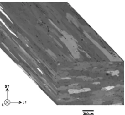
Figure1shows an optical microscope observation of the elon-gated grain structure of the 2024T351 rolled plate under polarized light. Before observation, the sample was mechanically polished with up to 4000 grit SiC papers and up to 1m with diamond paste on the three characteristic planes and then etched. Electrochemical etching was conducted with HBF4共3.5 vol. %兲 in distilled water for
80 s 共twice 40 s兲 under 20 V at room temperature. The average grain sizes in the longitudinal共L兲, long transverse 共LT兲, and short transverse共ST兲 directions were 700, 300, and 100 m, respectively. In addition, a combination of optical microscopy, scanning electron microscopy共SEM兲, and transmission electron microscopy observa-tions revealed a multiphase microstructure in the 2024 T351 alumi-num alloy consisting in共i兲 precipitates of second-phase Al2CuMg
particles共S phase particles兲 共ii兲 Al–Cu–Mn–Fe particles 共iii兲 disper-soids共Al20Mn3Cu兲 in the matrix, and 共iv兲 Al2CuMg particles on
grain boundaries. These observations present fair agreement with the results found in the literature.13
Current–potential curves.— Potentiokinetic polarization tests were performed using a conventional three-electrode cell at room temperature in aerated NaCl solutions for different chloride concen-trations, i.e., 0.5, 1, 3, and 5 M. The 1 M concentration corresponds
to a common chloride content for intergranular corrosion tests. A 5 M chloride solution was studied to reproduce the chemical condi-tions obtained after immersion–emersion cycling which regularly happens during the service life of an aircraft. A saturated calomel electrode共SCE兲 was used as a reference electrode and a platinum network as an auxiliary electrode. Potentiokinetic polarization ex-periments were conducted from the cathodic potential of −900 to the highest potential of −400 mV/SCE at a scan rate of 500 mV h−1.
The exposed surface of the working electrode共2024 aluminum alloy sample兲 corresponds to the LT–ST plane. At least three current– potential curves were plotted for each experimental condition to check the reproducibility of the measurements. In the manuscript, representative curves are given.
Intergranular corrosion tests.— Two types of sample geometries were considered: cubic samples共10 ⫻ 10 ⫻ 10 mm兲 used for con-ventional immersion tests and flat tensile specimens for mechanical tests. Before corrosion tests, both types of samples were degreased in ethanol, then mechanically polished with up to 4000 grit SiC paper in water, followed by ultrasonic cleaning in ethanol and air drying. The detailed description of the two types of samples and the surface preparation before corrosion tests has been given in a previ-ous paper.12Both types of samples were then exposed to aerated NaCl solutions at four different concentrations共0.5, 1, 3, and 5 M NaCl兲. The solution was maintained at room temperature 共25 ⫾ 2兲°C in a water bath. Exposure time varied from 12 to 3000 h. After exposure, cubic samples were sectioned perpen-dicularly to the corroded faces 共LT–ST plane兲 to be observed by optical microscopy. To take into account the random nature of the corrosion processes which is a well-known feature, all the inter-granular defects propagating in the rolling direction were counted and their depths measured.12For each experimental condition, at least four sections共L–ST plane兲 were observed which corresponded to a minimum of 4 cm of material analyzed in the ST direction with defects about 100m long for a mean value, i.e., a minimum of 4 mm2analyzed. Furthermore, SEM observations of several samples
were performed to check that optical microscopy was powerful enough to accurately detect the intergranular defects and to measure their depth. The results were then analyzed statistically. A prelimi-nary study was performed to determine the best method to calculate the mean depth. Results showed that the mean depth had to be calculated by taking into account the logarithm of the individual values.
Tensile tests.— Uncorroded tensile samples were tested to estab-lish the reference curve using a 30 kN Instron 3367 machine. After exposure to chloride solutions, the corroded tensile specimens were subjected to mechanical testing using the same test parameters. The tensile tests were carried out with an imposed displacement rate of 22⫻ 10−3mm s−1with a gage length of 22 mm corresponding to a
strain rate of 10−3s−1. The tests were pursued up to the failure of the
tensile specimens stressed along the ST direction. Elongation 共per-cent兲 was calculated from the ratio between the relative displace-ment and the initial gage length.
Results and Discussion
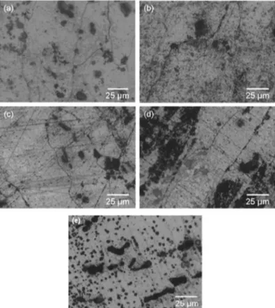
Determination of the application range of the T2C procedure.— Preliminary electrochemical tests.— Figure 2apresents potentioki-netic polarization curves for 2024 T351 aluminum alloy in 0.5, 1, 3, and 5 M NaCl solutions. For 0.5 and 1 M chloride concentrations, the curves exhibit only one breakdown potential corresponding to the corrosion potential, followed by a sharp increase of the anodic current density which can be related to corrosion phenomena. Opti-cal observations of the electrode after electrochemiOpti-cal tests at chlo-ride concentrations of 0.5 and 1 M showed that this breakdown potential was associated to localized corrosion on 2024 aluminum alloy: pitting and intergranular corrosions were observed at the end of the electrochemical tests共Fig.3aandb兲. The initiation potentials for pitting and intergranular corrosions were different but it was not Table I. Chemical composition of 2024 T351 aluminum alloy (wt
%).
Al Cu Mg Mn Fe Si Ti
%
共weight兲 Base 4.464 1.436 0.602 0.129 0.057 0.030
Figure 1. Optical view of a 2024 T351 rolled plate after electrochemical
possible to observe this feature with these current–potential curves. Independent of chloride concentration, a well-defined plateau corre-sponding to oxygen reduction was observed in the cathodic range. The cathodic current densities共in absolute values兲 decreased as the chloride concentration increased from 6⫻ 10−5to 1
⫻ 10−5A cm−2for 0.5 and 5 M chloride solutions, respectively. A
close-up of the cathodic part of the curves is given for clarity共Fig. 2b兲. This result can be easily explained taking into account the de-crease of the oxygen solubility with the inde-crease of chloride concen-tration as reported by Millero et al.14These authors showed that oxygen solubility in chloride solutions was equal to 223, 195, 110,
and 77mol 共kg H2O兲−1 for chloride contents of 0.5, 1, 3, and
5 M, respectively; it can be seen that the ratio between the oxygen content in chloride solutions and various chloride concentrations was well-correlated to the ratio between the cathodic current densi-ties measured on the oxygen reduction plateau for the corresponding solutions.
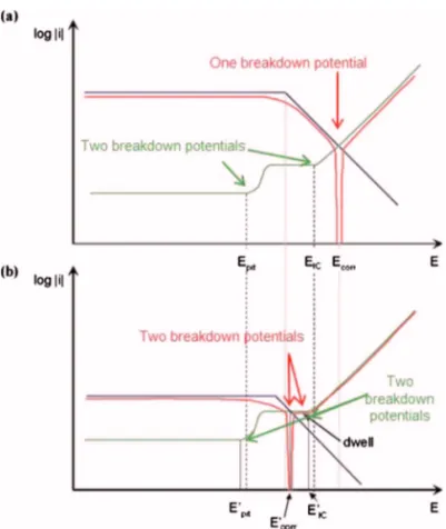
The decrease of the cathodic current densities when the chloride concentration increased could partially explain the shift of the cor-rosion potential toward more cathodic values; the corcor-rosion potential was actually shifted from −0.6 to − 0.88 V/SCE for 0.5 and 5 M chloride solutions, respectively. Moreover, this could also partially explain that the general shape of the current–potential curves was significantly modified since two breakdown potentials were ob-served for 3 and 5 M chloride solutions. Figure2cshows a close-up of the two breakdown potentials observed on the current–potential curves. The first breakdown potential corresponded to the corrosion potential as for 0.5 and 1 M NaCl solutions. The second breakdown potential, corresponding to the highest anodic potentials, is not as well-defined as the corrosion potential共first breakdown potential兲 and is preceded by a short plateau with anodic current densities too high to be attributed to passivity. Optical observations of the elec-trode after the electrochemical tests revealed pitting and intergranu-lar corrosions共Fig.3candd兲. Optical observations of the electrode surface for an interrupted test at −0.78 V/SCE 共between the two breakdown potentials兲 in a 5 M chloride solution exhibited only pitting corrosion, except intermetallic particle dissolution共Fig.3e兲. Therefore, for 3 and 5 M chloride solutions, the first breakdown potential共corrosion potential兲 was thus attributed to pitting corro-sion while the more anodic was related to intergranular corrocorro-sion. Of course, the first breakdown potential共corrosion potential兲 also took into account an anodic contribution corresponding to interme-tallic particle dissolution, but it was not possible to differentiate the two phenomena.13Moreover, comparison of the curves plotted for 3 and 5 M chloride solutions showed that the second breakdown po-tential, i.e., the potential corresponding to initiation of intergranular
Figure 2.共Color online兲 共a兲 Current–potential curves for 2024 T351
alumi-num alloy in 0.5, 1, 3, and 5 M NaCl solutions at 25°C. Scan rate = 500 mV h−1.共b兲 Close-up of the cathodic parts of the curves; 共c兲 Close-up
of the anodic parts of the current–potential curves; vertical lines show the breakdown potentials.
Figure 3. Optical observations of corroded faces on 2024 T351 aluminum
alloy after potentiokinetic polarization in共a兲 0.5, 共b兲 1, 共c兲 3, and 共d兲 5 M NaCl solutions and共e兲 for an interrupted potentiokinetic polarization test at −780 mV/SCE in a 5 M NaCl solution at 25°C.
corrosion damage, was shifted toward more cathodic potentials for a chloride content of 5 M共Fig.2c兲. This was attributed to the aggres-sion of chloride ions toward 2024 aluminum alloy. By analogy, it was assumed that the potential corresponding to pitting initiation was also shifted toward more cathodic values as chloride concentra-tion increased.15,16The influence of chloride content on the suscep-tibility of the 2024 aluminum alloy to localized corrosion contrib-uted to explain the shift of the corrosion potential toward more cathodic values when the chloride concentrations increased. To sum up the effect of the chloride content, Fig. 4presents a schematic view of the potentiokinetic polarization curves for low and high chloride contents. It is important to recall here that the current– potential curves described previously result from the addition of cathodic currents共elementary cathodic curve兲 and anodic currents 共elementary anodic curve兲 and, depending on the relative positions of the elementary curves, the resulting current–potential curves will be different. In particular, the breakdown potentials identified on the elementary curves can be visible or not and/or shifted on the result-ant current–potential curves. In Fig. 4, the elementary cathodic curve, corresponding to the oxygen reduction reaction, is commonly represented by a diffusion plateau followed by a Tafel straight line. The elementary anodic curve is more complex. After the passivity plateau, a first breakdown potential was observed due to the initia-tion of pitting corrosion and intermetallic particle dissoluinitia-tion. A plateau with high anodic current densities was then observed due to pit propagation and intermetallic dissolution. The second breakdown potential was previously attributed, from experimental observations 共the second breakdown potential of the elementary anodic curve was directly visible, with a slight shift, on current–potential curves only for those plotted for 3 and 5 M solutions兲, to intergranular corrosion initiation. As deduced from experimental results, the potentials cor-responding to the initiation of pitting and intergranular corrosions
were shifted toward more cathodic values as the chloride concentra-tion increased. Moreover, the oxygen reducconcentra-tion plateau was lower for high chloride concentrations due to low oxygen solubility. It was also assumed that the anodic plateau corresponding to pit propaga-tion was higher for high chloride concentrapropaga-tions since it was ob-served that the density and the size of the pits increased as chloride concentrations increased共Fig.3兲. Therefore, the anodic contribution was significant just before the corrosion potential for high chloride contents which explained the slope observed on the cathodic plateau for high chloride contents and mainly for a 5 M chloride solution 共Fig.2b兲.
Finally, these tests showed that at the corrosion potential, 2024 alloy presented pitting and intergranular corrosions at low chloride concentrations but only pitting corrosion at high chloride concentra-tions. However, the potential scan rate was very high, and thus the electrochemical conditions imposed on the electrode most likely did not correspond to an equilibrium state. Therefore, intergranular cor-rosion will be observed at the corcor-rosion potential during immersion tests whatever be the concentration, but significant differences might be revealed concerning the density and the size of the intergranular corrosion defects.
Intergranular immersion tests.— Figure 5 shows optical micro-graphs obtained on 2024 alloy after different immersion times, i.e., 24, 72, and 168 h in 0.5, 3, and 5 M NaCl solutions. Intergranular corrosion was observed on all samples with an increased depth of corrosion attack when immersion time increased independent of chloride concentration. We also observed an increase of the opening of the attacks with immersion time but this was mainly evidenced for 0.5 M NaCl concentration. In this case, after 168 h, the size of intergranular defects was about 300m in depth and more than 50m in opening. For 3 and 5 M chloride concentrations, the in-tergranular defects were narrow: for a given immersion time, the opening of intergranular defects decreased with increasing chloride concentrations. So, intergranular attack morphology was signifi-cantly influenced by chloride concentration.
As mentioned in the experimental part, to take measurement scatter into account, four sections were observed for all chloride concentrations and immersion times. For each section, all the inter-granular defects propagating in the rolling direction were counted and their depths were measured. This is a sufficient number to en-able statistical analysis of the results.12Figure6apresents the aver-age depth of intergranular defects versus immersion time for differ-ent chloride concdiffer-entrations. Globally, average depths increased along with the immersion time for a given chloride concentration. Moreover, for a given immersion time greater than 24 h, average depths increased along with chloride concentration. However, for immersion times shorter than 24 h, the number of intergranular de-fects was so low for 5 M chloride concentration that it was not possible to evaluate their mean depth. This observation shows that corrosion defect density was a relevant parameter to describe corro-sion damage.
Figure6bshows the density of intergranular damage sites versus immersion time for different chloride concentrations. The density is calculated as the ratio between the number of grain boundaries cor-roded and the total number of grain boundaries counted on the sec-tion analyzed. For a given chloride concentrasec-tion, the density of intergranular damage increased with immersion time. Moreover, it clearly appears that the density of intergranular defects decreased when chloride concentration increased, particularly for short immer-sion times.
These tests seem to show that intergranular corrosion defect ini-tiation was easier at low than at high chloride concentrations. This was not consistent with potentiokinetic polarization results and es-pecially with the shift of the second breakdown potential toward more cathodic potentials when chloride concentrations increased. This was explained by taking into account the two steps of inter-granular corrosion, i.e., initiation and propagation, and it was as-sumed that when chloride concentration increased, intergranular cor-rosion initiated more easily as shown by the potential shift on the
Figure 4.共Color online兲 Schematic effect of chloride ion concentration on
potentiokinetic polarization curves on 2024 T351 aluminum alloy for:共a兲 low chloride concentrations共0.5 and 1 M兲 and 共b兲 high chloride concentra-tions共3 and 5 M兲; in green the anodic segment 共breakdown potentials shown with green arrows兲, in blue the cathodic segment, and in red the global potentiokinetic curve共breakdown potentials shown with red arrows兲.
potentiokinetic polarization curves but only a few intergranular de-fects could propagate enough to be detected. This was due to the low oxygen solubility and to the fact that in chloride media, 2024 alu-minum alloy presented a competition between two types of corro-sion mechanisms: pitting and intergranular corrocorro-sions. For high chloride concentrations, 2024 alloy presented more numerous and bigger pits which led to an evolution of the morphology of inter-granular corrosion defects: they became less numerous, thinner, but deeper as the chloride concentration increased.
It can be noticed that a low intergranular defect density increased the error on the measurement of defect depth. This point has been discussed in a previous paper.12Determination of the propagation kinetics of intergranular defects by sectioning and observing precor-roded samples requires a very large number of samples to be mean-ingful. Such a method is thus highly time consuming and, with a reasonable number of samples, it allows only descriptive results to be obtained. Hence a new method was envisaged based on the load to failure on precorroded tensile specimens versus immersion time in aggressive media.
Validation of the T2C procedure for different chloride concentra-tions and immersion times.— As recalled in the introduction, this method assumes that a homogeneous distribution of corrosion dam-age over the whole surface of a tensile precorroded specimen leads to the presence in the material of a nonbearing zone. As the effective bearing area is decreased, the load to failure for a corroded specimen will decrease too. Following this assumption, the propagation of intergranular corrosion can be considered as the growth of the thick-ness of the nonbearing zone along the whole length of the tensile specimens. More details about this method are given in a previous paper.12The method has already been successfully used to deter-mine the mean depth of intergranular defects for chloride concentra-tions of 1 and 3 M and immersion times no longer than 168 h.12It is important to bear in mind that the geometry of the tensile specimens was chosen in order to provide a large enough analyzed corroded surface to obtain relevant measurements for the mean depth of in-tergranular defects. Moreover, for each experimental condition, at least, three tensile specimens were studied. Figure7shows the mean depth of intergranular defects determined using this method for chloride concentrations of 0.5, 1, 3, and 5 M and immersion times up to 168 h. The results are indicated by continuous lines. The mean
depths of intergranular defects calculated from conventional immer-sion tests are reported for comparison共dashed lines兲. These results show a good agreement between the two sets of values for chloride concentrations up to 3 M. However, measurements calculated by tensile tests共T2C procedure兲 are underestimated for a 5 M chloride
concentration. This last observation can be easily explained by tak-ing into account the error on the measurement of intergranular de-fect depth in highly concentrated chloride solutions for both meth-ods, i.e., T2C procedure and conventional immersion tests: for the T2C procedure, the intergranular defect density was too low for a
nonbearing zone to be defined, while for conventional immersion tests, the intergranular defect density was too low for a statistical analysis to be performed. The T2C procedure was thus an efficient method to determine the mean intergranular defect depth for chlo-ride concentrations, leading to a homogeneous distribution of inter-granular defects, i.e., for the concentration range studied in this work, for concentrations up to 3 M. It also proved that the longest defects were not so damaging in terms of global mechanical re-sponse of the specimen. This observation suggests that the geometry of these defects cannot be considered as cracks; otherwise, the lo-cally restricted deformation would make the T2C analysis
inappro-priate.
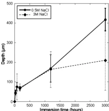
Additional experiments were then performed to evaluate whether it was possible to use the T2C procedure for immersion times as
long as 3000 h. Figure8presents the average intergranular defect depth calculated from tensile tests on precorroded specimens versus immersion time for 0.5 and 3 M chloride solutions and for immer-sion times from 0 to 3000 h. Whatever the chloride concentration, the average depth of intergranular defects increased with immersion time with two intergranular corrosion kinetics regimes: during the first 200 h, intergranular corrosion propagated very rapidly, whereas for longer immersion times, the propagation kinetics of intergranular corrosion was found to be lower which was significant mainly for a 3 M chloride solution. The results were in good agreement with those obtained by Pauze who showed the existence of two inter-granular corrosion kinetics regimes in NaCl solutions: during the first 7 h of immersion, a fast intergranular corrosion regime 共30 m/h兲 and then from 7 to 12000 h of immersion, a slow regime 共0.06 m/h兲.17
The author explained the results by referring to mi-Figure 5. Optical micrographs of
inter-granular corrosion defects on 2024 T351 aluminum alloy after immersion in 0.5, 3, and 5 M NaCl solutions for 24, 72, and 168 h at 25°C.
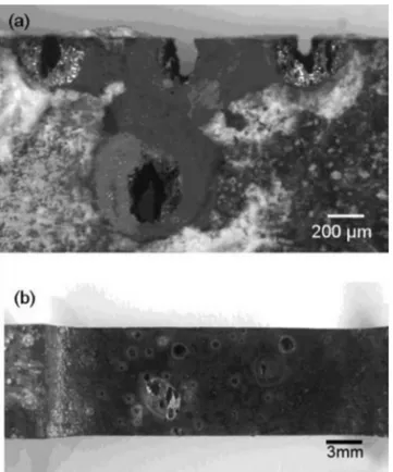
crostructural effects such as grain morphology or electrochemical parameters such as a decrease of the oxygen concentration at the defect tip. Moreover, it was possible that an ohmic loss between the interior and the exterior of the corrosion defect could be responsible for the existence of these two kinetic regimes.17However, Fig. 8 shows that the values of intergranular corrosion defect depth were very scattered 共for each condition, the deviation between the ten measurements is reported for the corresponding average values兲 for immersion times of 1200 and 3000 h with an increased scattering with increasing immersion time. Optical micrographs of corroded samples after 3000 h of immersion in 0.5 and 3 M NaCl solutions are presented in Fig.9. Very large defects were detected for both chloride concentrations with some defects passing through the cor-roded sample; analysis showed the red corrosion product to be com-posed of copper species. Such defects were also observed on samples immersed for 1200 h, but they were much less numerous and their morphology was more similar to that observed for short
immersion times, i.e., a homogeneous distribution of intergranular corrosion defects. Analysis of the load/elongation curves obtained for precorroded samples in 0.5 or 3 M chloride solution showed that whereas the curves obtained for ten samples precorroded for a given immersion time up to 1200 h were reproducible, those obtained for ten samples immersed in a given solution for 3000 h were very scattered共Fig.10兲. In Fig.10, the ten gray curves correspond to ten tensile tests performed for ten samples precorroded in the same con-ditions共same solution and same immersion time兲. The black curve corresponds to a tensile test performed on a noncorroded sample for comparison. This result was related to the corrosion morphology. Immersion in chloride solutions for very long time, i.e., 3000 h led to the growth of very large corrosion cavities whose geometrical
Figure 8. Calculated average depth共T2C procedure兲 of intergranular damage
vs immersion time for 2024 T351 aluminum alloy for 0.5 M共continuous lines兲 and 3 M 共dashed lines兲 NaCl solutions at 25°C.
Figure 6.共Color online兲 共a兲 Average depth of intergranular damage vs
im-mersion time in 2024 T351 aluminum alloy for 0.5, 1, 3, and 5 M NaCl solutions at 25°C;共b兲 Ratio of damaged sites to potential sites vs immersion time for 2024 T351 aluminum alloy in 0.5, 1, 3, and 5 M NaCl solutions at 25°C.
Figure 7. 共Color online兲 Calculated 共T2C procedure: continuous lines兲 and
measured共conventional immersion tests: dashed lines兲 average depth of in-tergranular damage vs immersion time in 2024 T351 aluminum alloy for 0.5, 1, 3, and 5 M NaCl solutions at 25°C.
characteristics共shape, size, distribution兲 were random. In such con-ditions, the corrosion damage could no longer be described as a nonbearing zone distributed along the whole length of the tensile specimens and the fracture of the tensile samples was directly re-lated to the geometrical characteristics of the corrosion cavities which explained the scattering of the load/elongation curves. The T2C procedure was thus unusable for long immersion times 共3000 h兲.
Therefore, the T2C procedure approved to be reproducible, fast,
and reliable for the calculation of the average depth of the inter-granular corrosion defects as long as interinter-granular defects are suffi-ciently numerous and lead to a homogeneous distribution of the damage observed for immersion times up to 1200 h and chloride concentrations up to 3 M. However, for longer immersion times 共 ⬎ 1200 h兲 and for higher chloride concentrations 共 ⬎ 3 M兲, the results deduced from classical immersion tests and from this T2C
procedure must be considered with caution. This is why empirical propagation laws of intergranular corrosion defects were determined using the T2C procedure for a maximum chloride concentration of 3 M and a maximum immersion time of 1200 h.
Empirical propagation laws of intergranular corrosion defects.— The T2C procedure was used to determine empirical propagation
laws of intergranular corrosion defects for 2024 T351 aluminum alloys in 0.5 and 3 M chloride solutions. Ten samples were tested for each condition to validate the empirical propagation law pro-posed. Figure11presents the average depth of intergranular corro-sion defects versus immercorro-sion time for chloride concentrations of Figure 9. Optical micrograph of corroded surfaces of 2024 T351 aluminum
alloy after 3000 h immersion in共a兲 a 0.5 M NaCl solution and 共b兲 a 3 M NaCl solution at 25°C.
Figure 10. Load vs elongation curves for 2024 T351 aluminum alloy
samples after 3000 h immersion in a 3 M NaCl solution at 25°C. Ten curves corresponding to the precorroded samples are given in gray to show the lack of reproducibility of the tensile test results. A curve in black is given for a reference sample共noncorroded sample兲 for comparison.
Figure 11. Calculated average depth共T2C procedure兲 of 2024 T351
alumi-num alloy samples immersed in共a兲 0.5 and 共b兲 3 M NaCl solutions for different immersion times at 25°C.
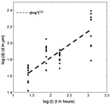
0.5 and 3 M. The shape of the intergranular corrosion defects propa-gation curves was similar for 0.5 and 3 M chloride concentration with two propagation regimes, which suggests a propagation power-law of the form d = atb, with a and b depending on environmental parameters and d corresponding to the average depth of the inter-granular corrosion defects. In the literature, most studies identify parabolic laws of the form d = at1/2with a˜ also depending on the direction of intergranular corrosion propagation.4,9 In the present work, this parabolic law does not fit the results as represented in Fig. 12in a log–log plot, particularly in the long immersion times range. In order to improve the prediction of intergranular corrosion propa-gation, a first attempt to propose another law was described here. This attempt is explained in the present paper only for a 0.5 M chloride concentration and will be transposed to 3 M NaCl condi-tions.
As shown in Fig.11, two regimes characterize corrosion defect propagation: during the first 200 h of immersion, a fast intergranular corrosion regime and, subsequently, from 200 to 1200 h of immer-sion, a stationary regime. For this regime, linear regression led to a formula of the type d = At + C共Fig.13兲, with A and C depending on environmental parameters. The formula calculated by linear re-gression was d = 0.07t + 55 with a correlation coefficient R equal to 0.48. Of course, this coefficient was low but this can be explained first by the strong dispersion of the intergranular defect depths ob-served at 1200 h. Moreover, it would be necessary to perform ex-periments for immersion times between 168 and 1200 h to improve the results, and maybe it would also be helpful to test more than ten tensile samples for each immersion times. However, the aim of the present work is to propose a first attempt to determine propagation kinetics of intergranular corrosion defects for 2024 alloy, and the formula d = 0.07t + 55 was taken as being representative of the stationary propagation regime from 200 to 1200 h. For the fast propagation regime, it was interesting to plot the variance between average depths calculated by the formula At + C versus measured average depths d for different immersion times: At + C − d 共Fig. 14兲. A strong dispersion was still logically observed for long immer-sion times. For short immerimmer-sion times, variance appeared to change following an exponential pattern. As most studies in the literature have shown that intergranular corrosion defect propagation depends on t1/2, this formula was considered.4,9As a consequence, the equa-tion describing the kinetics of intergranular corrosion defect propa-gation was of the type d = At + C共1 − exp共−Bt1/2兲兲, where A, B,
and C depended on environmental conditions. So, calculations gave two empirical propagation laws for 0.5 and 3 M chloride concentra-tions:
NaCl 0.5 M d = 0.07t + 55共1 − exp共− 0.2t1/2兲兲 NaCl 3 M d = 0.09t + 66共1 − exp共− 0.14t1/2兲兲
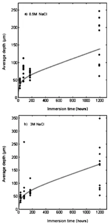
Figure15presents a comparison between average depths calculated by empirical propagation laws and measured average depths for 0.5 Figure 12. Representation of the kinetics of intergranular corrosion defect
propagation as a log–log plot for a 0.5 M chloride solution. d corresponds to the average depth of the intergranular corrosion defect.
Figure 13. Linear regression of stationary propagation regime in a 0.5 M
chloride solution.
Figure 14. Intergranular corrosion defect propagation关d corresponds to the
average depth of the intergranular corrosion defect兴 and variance At + C − d vs immersion time.
and 3 M chloride concentrations. Given the strong dispersion of results of intergranular corrosion damage, experimental and calcu-lated curves presented a good agreement. Therefore, equation d = At + C共1 − exp共−Bt1/2兲兲 can suitably describe intergranular
cor-rosion defect propagation, where A, B, and C depend on chloride concentration. To improve these empirical propagation laws, it would be necessary to perform experiments for other values of the immersion time between 200 and 1200 h.
Conclusion
In this work, the intergranular corrosion susceptibility of 2024 T351 aluminum alloy was studied. The results indicate that measur-ing intergranular corrosion defect propagation by means of the load to failure on precorroded tensile samples 共T2C procedure兲 was a
relevant alternative method to classical immersion and sectioning tests in corrosive environments for chloride concentrations up to 3 M and immersion times up to 1200 h. For these experimental conditions, it was shown that intergranular corrosion led to the growth of a nonbearing zone of thickness equal to the mean depth of the corrosion defects. For higher chloride concentrations, due to high pit density, the intergranular corrosion defect density was too low to generate a nonbearing zone and thus the T2C procedure was unusable. For longer immersion times共 ⬎ 1200 h兲, corrosion dam-age was no longer intergranular but took the form of very large cavities whose geometrical characteristics were difficult to describe due to their random nature. For these reasons, empirical propagation laws of intergranular corrosion defects in NaCl solutions were es-tablished using the T2C procedure only for immersion times of up to
1200 h and for chloride concentrations up to 3 M. Empirical laws accurately described corrosion kinetics measurements for these ex-perimental conditions. This first calculation step will be the basis for future and more complex predictive corrosion damage laws for the aeronautic industry.
Acknowledgments
This work was supported by EADS Innovation works and Direc-tion Générale de l’Armement共DGA兲. The authors thank Maurice Sarfati from DGA for fruitful discussions.
Centre National de la Recherche Scientifique assisted in meeting the publication costs of this article.
References
1. Z. Szklarska-Smialowska, Corros. Sci., 41, 1743共1999兲.
2. J. W. J. Silva, A. G. Bustamante, E. N. Codaro, R. Z. Nakazato, and L. R. O. Hein,
Appl. Surf. Sci., 236, 356共2004兲.
3. A. Garner and D. Tromans, Corrosion (Houston), 35, 55共1979兲.
4. X. Zhao, G. S. Frankel, B. Zoofan, and S. Rokhlin, Corros. Sci., 59, 1012共2003兲. 5. M. Posada, L. E. Murr, C. S. Niou, D. Roberson, D. Little, R. Arrowood, and D.
George, Mater. Charact., 38, 259共1997兲. 6. M. R. Bayoumi, Eng. Fract. Mech., 54, 879共1996兲.
7. X. Liu, G. S. Frankel, B. Zoofan, and S. Rokhlin, Corros. Sci., 49, 139共2007兲. 8. W. Zhang and G. S. Frankel, Electrochem. Solid-State Lett., 3, 268共2000兲. 9. W. Zhang and G. S. Frankel, J. Electrochem. Soc., 149, 510共2002兲.
10. W. Zhang, S. Ruan, D. A. Wolfe, and G. S. Frankel, Corros. Sci., 45, 353共2003兲. 11. T. Huang and G. S. Frankel, Corros. Sci., 49, 858共2007兲.
12. C. Augustin, E. Andrieu, C. Blanc, G. Mankowski, and J. Delfosse, J. Electrochem.
Soc., 154, 11共2007兲.
13. V. Guillaumin and G. Mankowski, Corros. Sci., 41, 421共1998兲. 14. F. J. Millero, F. Huang, and A. L. Laferiere, Mar. Chem., 78, 217共2002兲. 15. J. Galvele and S. De Micheli, Corros. Sci., 10, 795共1970兲.
16. F. Dabosi, G. Béranger, and B. Baroux, in Corrosion Localisée, Les Editions de Physique, Les Ulis Cedex A, France共1994兲.
17. N. Pauze, Ph.D. Thesis, Ecole Nationale Supérieure des Mines de Saint-Etienne, 2008.
Figure 15. Comparison between average intergranular corrosion defect
depth calculated by empirical propagation laws共lines兲 and measured average depths for共a兲 0.5 and 共b兲 3 M chloride concentrations 共points兲.