HAL Id: hal-01164873
https://hal.archives-ouvertes.fr/hal-01164873
Submitted on 18 Jun 2015
HAL is a multi-disciplinary open access
archive for the deposit and dissemination of
sci-entific research documents, whether they are
pub-lished or not. The documents may come from
teaching and research institutions in France or
abroad, or from public or private research centers.
L’archive ouverte pluridisciplinaire HAL, est
destinée au dépôt et à la diffusion de documents
scientifiques de niveau recherche, publiés ou non,
émanant des établissements d’enseignement et de
recherche français ou étrangers, des laboratoires
publics ou privés.
Propagation of Intergranular Corrosion Defects in AA
2024-T351 Evaluated by a Decrease in Mechanical
Resistance
Céline Larignon, Joël Alexis, Eric Andrieu, Grégory Odemer, Christine Blanc
To cite this version:
Céline Larignon, Joël Alexis, Eric Andrieu, Grégory Odemer, Christine Blanc. Propagation of
In-tergranular Corrosion Defects in AA 2024-T351 Evaluated by a Decrease in Mechanical Resistance.
Journal of The Electrochemical Society, Electrochemical Society, 2014, vol. 161 (n° 6), pp.C339-C348.
�10.1149/2.090406jes�. �hal-01164873�
O
pen
A
rchive
T
OULOUSE
A
rchive
O
uverte (
OATAO
)
OATAO is an open access repository that collects the work of Toulouse researchers and
makes it freely available over the web where possible.
This is an author-deposited version published in :
http://oatao.univ-toulouse.fr/
Eprints ID : 14066
To link to this article : doi:
10.1149/2.090406jes
URL :
http://dx.doi.org/10.1149/2.090406jes
To cite this version : Larignon, Céline and Alexis, Joël and Andrieu,
Eric and Odemer, Grégory and Blanc, Christine Propagation of
Intergranular Corrosion Defects in AA 2024-T351 Evaluated by a
Decrease in Mechanical Resistance. (2014) Journal of The
Electrochemical Society, vol. 161 (n° 6). C339-C348. ISSN 0013-4651
Any correspondance concerning this service should be sent to the repository
administrator:
[email protected]
Propagation of Intergranular Corrosion Defects in AA 2024-T351
Evaluated by a Decrease in Mechanical Resistance
C´eline Larignon,aJo¨el Alexis,bEric Andrieu,aGr´egory Odemer,aand Christine Blanca,∗,z
aUniversit´e de Toulouse, CIRIMAT, UPS/CNRS/INPT, 31030 Toulouse Cedex 04, France bUniversit´e de Toulouse, LGP, ENIT, 65016 Tarbes Cedex, France
This study deals with propagation kinetics of intergranular corrosion defects. It complements previous works focused on the development of a procedure called “T2C (Tensile Test for Corrosion).” This procedure was previously applied on samples of 2024 alloy submitted to a continuous immersion test in 1 M NaCl solution. The aim of the present study was to determine if a modification in the way in which the samples are corroded impacts the ability to use this procedure. Therefore, the applicability of the T2C procedure to cyclic corrosion tests was evaluated. Intergranular corrosion defects developed during cyclic corrosion tests were characterized by using a statistical approach. The geometry of the tensile specimens was optimized to allow the T2C procedure to be applied in conditions expected as adequate. Results showed that, for cyclic corrosion tests, due to the branched morphology of the intergranular corrosion defects and the effects of hydrogen embrittlement, the T2C procedure cannot provide an estimation of the mean depth of the intergranular corrosion defects. However, depending on the cyclic corrosion tests, it allowed the maximal depth of the intergranular corrosion defects or the thickness of the corrosion-induced damage zone (defects + hydrogen affected zone) to be determined.
DOI:10.1149/2.090406jes
High strength aluminum alloys such as 2xxx series alloys and espe-cially AA2024-T351 are widely used in the aircraft industry because of their good mechanical properties and their low density. However, these alloys are known to be susceptible to localized corrosion such as pitting corrosion,1–3 intergranular corrosion,4–6 exfoliation,7,8 and
stress corrosion cracking.9,10Intergranular corrosion is considered a
major threat to the structural integrity of aircraft structures but, to-day, intergranular corrosion propagation and its impact on structural integrity is still uncertain and therefore it is not easy to include these data in the damage tolerance concept. Therefore, it is of interest to increase the knowledge concerning the kinetics for the propagation of intergranular corrosion defects. A first step for such a predictive approach of the lifetime of aircrafts is to provide data about the ki-netics at least under controlled conditions, i.e. at the laboratory scale. However, to be reached, this objective requires the development of an experimental approach allowing characterization of the intergranular corrosion damage and providing data concerning both the intergran-ular corrosion defects themselves (size, distribution) and a possible volume damage associated with these defects. Indeed, Kamoutsi et al. provided clear evidence of corrosion-induced hydrogen embrittle-ment in aluminum alloy 2024 and showed that the decrease of the mechanical properties for a corroded sample included both the effect of the corrosion defects and that of hydrogen.11,12
Many authors have used a variety of methods to study inter-granular corrosion damage growth and propose propagation laws. For example, Zhang and Frankel used the foil penetration technique on a 2024-T3 aluminum alloy to measure the time required for the fastest growing corrosion sites to penetrate through foils of various thicknesses.13,14 They observed strong anisotropy in the growth
ki-netics of damage, with slower propagation observed in the short transverse (ST) direction compared with either the long transverse (LT) or the rolling/longitudinal (L) directions. According to these authors, this kinetic anisotropy is directly related with the microstruc-tural anisotropy, which is determined by both grain size and aspect ratio. In a later report, they continued this investigation by devel-oping a statistical model for intergranular corrosion propagation to explain the differences observed in corrosion growth kinetics and the impact of the microstructure.15Huang and Frankel developed an
ap-proach based on visual observations of serial cross sections along the corrosion propagation direction to determine the kinetics of sharp intergranular corrosion cracks in AA7178, monitoring not only the growth rates of long intergranular corrosion cracks but also the rates of the fastest growing sites.16
zE-mail:[email protected]
The methods described above have several limitations, including the fact that neither the random nature of the intergranular corro-sion defect propagation nor the three-dimencorro-sional morphology of the corrosion defects are taken into account. Additionally, the main pa-rameter responsible for the damage has not yet been identified, with the fastest growing defects or the mean depth of all corrosion defects as two possibilities. Furthermore, only data concerning the corrosion defects are obtained without considering the presence of a possible volume damage. Augustin et al. characterized the intergranular cor-rosion of the 2024-T351 aluminum alloy after continuous immersion in 1 M and 3 M chloride media by using optical microscopy observa-tions of corroded sample cross secobserva-tions.17These observations allowed
determination of a statistical value of the mean depth of the intergran-ular corrosion defects but this method was time consuming because it requires observation of a large number of cross sections to provide representative results. Thus, in the same work, the authors explored another method to estimate the depth of the corrosion defects. This method, called the Tensile Test for Corrosion (T2C) procedure, was based on the evolutions in the mechanical response, particularly the load to failure and the flow stress, between corroded and non-corroded tensile specimens. Because, with the exposure conditions tested (con-tinuous immersion in 1 M and 3 M NaCl solution), the intergranular corrosion defects were statistically distributed along the gauge length of the tensile specimen, the authors assumed that the corroded zone of the sample could be simplified to the development of a mechanically non-load-bearing zone. This approach supposed that the load-bearing zone behaved as a thinner tensile specimen provided that the metallur-gical state of the bulk material remained unaffected by the corrosion processes, e.g. hydrogen embrittlement. With this assumption, this method allowed for easier and more rapid determination of the ge-ometric mean depth of the corrosion attack than optical microscopy observations. As this method yielded good results for chloride con-centrations of 1 M and 3 M and for immersion times up to 168 h, the authors tested the procedure for a larger range of concentration from 0.5 M to 5 M and for longer immersion times up to 3000 h to define the applicability limits of this new method.18A 5 M concentration
was close to the saturation concentration; it could be considered as representative of the chloride content of the electrolyte trapped inside the corrosion defects under alternate immersion-emersion corrosion tests.19,20The results of this second study indicated that the T
2C pro-cedure was relevant for NaCl concentrations from 0.5 M to 3 M and for immersion times no longer than 1200 h.
However, the previous studies were based on continuous immer-sion tests, while aircraft structures are cyclically exposed to corrosive environments, with the plane exposed to a corrosive environment on the tarmac but not during a flight. Furthermore, in flight, some parts of
Table I. Chemical composition of the 2024 T351 aluminum alloy (wt%).
Alloying element Al Cu Mg Mn Fe Si Ti % weight Base 4.464 1.436 0.602 0.129 0.057 0.030
the structure drop to roughly −50◦
C, while other parts remain at room temperature. Larignon et al. showed that cyclic exposure affected the morphology of intergranular corrosion defects and generated a signif-icant hydrogen embrittlement effect.19–23
Based on these previous results, the present paper focuses on the application of the T2C procedure to cyclic corrosion tests that cor-respond to corrosion conditions closer to those actually encountered in the aircraft industry. The aim was to assess the effect of both the intergranular corrosion defects and the hydrogen-enriched zone on the mechanical response of the corroded samples to evaluate the inter-est of the T2C procedure for such corrosion tests. The first part of the manuscript is devoted to characterization by optical microscopy of the intergranular corrosion defects due to cyclic corrosion tests. Based on those results, the second part of the manuscript aims to determine the optimal thickness of the tensile specimen to detect the non-bearing zone generated by the corrosion defects. In the third part of the study, the applicability of the T2C procedure for cyclic corrosion tests is studied.
Experimental
Material.—Experiments were performed on a 2024 T351 alu-minum alloy supplied in the form of a 50 mm thick rolled plate. The chemical composition of the alloy is presented in TableI. The T351 temper consists of a solid-solution heat-treatment at 495◦
C (±5◦ C) followed by water quenching, straining (1 to 2%) and tempering in ambient conditions for four days. The microstructure of this material consists of grains elongated in the longitudinal direction (L). Aver-age grain sizes in the longitudinal, long transverse (LT) and short transverse (ST) directions were 700, 300 and 100 µm, respectively. Observations using an optical microscope (OM), a scanning electron microscope with a field emission gun (SEM-FEG) and transmission electron microscopy (TEM) showed both intragranular precipitates, such as Al-Cu-Mn-Fe and Al2CuMg particles, and intergranular pre-cipitates (mainly Al2CuMg and Al-Cu-Mn). No precipitate-free zone (PFZ) was observed along the grain boundaries in the as-received plate. These observations are in good agreement with the literature.6
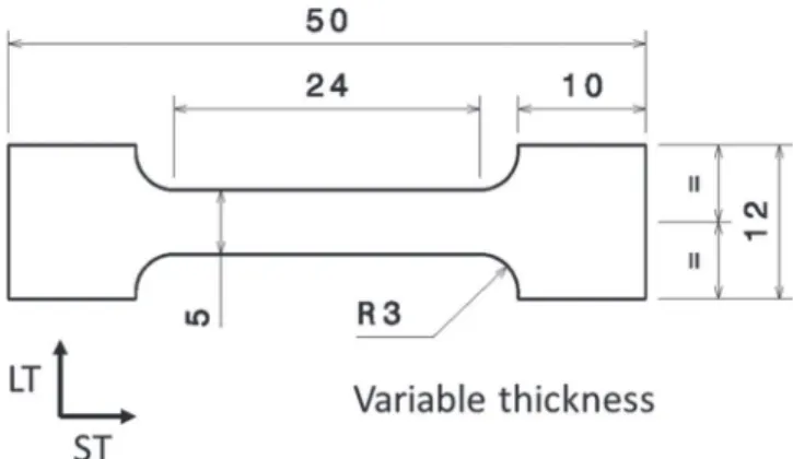
Intergranular corrosion tests.—Both continuous immersion tests and cyclic corrosion tests (alternate immersion-emersion tests) were performed (TableII). For all the corrosion tests, the electrolyte was a 1 M NaCl solution prepared with Rectapur chemicals dissolved in distilled water. Tests were carried out on both cubic samples (10 mm edge) to observe and characterize the intergranular corrosion defects and on tensile specimens (Figure1) to test the applicability of the T2C
Figure 1. Geometry of the tensile specimens (all dimensions in mm).
procedure. The thickness of the tensile specimens in the L direction was a variable used to improve the applicability of the T2C procedure (see the results and discussion part): it was varied from 1.2 mm to 12 mm. All samples were extracted from the core of the plate. For tensile specimens, if no more details are given in the manuscript, both the LT-ST and ST-L planes of the tensile specimens were exposed to the electrolyte; the mechanically bearing section was the LT-L plane with corrosion defects propagating mainly in the L direction which was the most critical direction for corrosion propagation. For cubic samples, the LT-ST plane was exposed to the electrolyte in order to observe and quantify the intergranular corrosion defects propagating in the L direction. Other planes were masked using a varnish. Independent of the corrosion tests, the same size of the samples was used and the same planes were exposed to the electrolyte. Before corrosion tests, the samples were degreased in ethanol, mechanically polished with different grit SiC papers up to 4000 grit grade, then rinsed in distilled water and air-dried. All corrosion tests were conducted in a laboratory room with controlled temperature (T = 22◦
C). The hygrometry was measured during the testing period (51% relative humidity). More-over, to avoid temperature fluctuations of the electrolyte due to the size of the laboratory room, the temperature of the electrolyte was also controlled and maintained at 25 ± 2◦C by using a thermostat-cryostat. Two cyclic corrosion tests were performed, both consisting of three 24 h cycles. Each cycle consisted of an 8 h immersion at room temperature in the electrolyte followed by a 16 h emersion in air at the temperature of the laboratory room i.e., 22◦
C for the Cyclic Room (CR) test and at −20◦
C for the Cyclic Freezing (CF) test. The duration of both the immersion and emersion phases was chosen to be com-patible with a work day. Furthermore, additional experiments using a microbalance were carried out to evaluate the time the electrolyte trapped inside the corrosion defects needed to evaporate during the air exposure periods at room temperature (CR tests). Results showed that it could be assumed that, even if corrosion defects could remain wet during the air exposure periods, the electrolyte evaporation was sufficient enough to partially dry the corrosion products and generate
Table II. Description of the corrosion tests.
Exposure conditions Continuous immersion
Description of the tests / Name of the tests Continuous immersion in 1 M NaCl (25 ± 2◦C) Duration 24 h: CI 24 h
Duration 72 h: CI 72 h
Exposure conditions Cyclic corrosion test = alternate immersion (1 M NaCl at 25 ± 2◦C) and emersion periods Description of the tests / Name of the tests 3 × (24 hour cycles)
a cycle = 8 hour immersion / 16 hour dry period Cumulative immersion time = 3 × 8 = 24 h Duration of the cyclic corrosion test = 3 × 24 = 72 h Temperature during the dry period
=22 ± 1◦C CR tests
Temperature during the dry period = −20 ± 1◦C
a concentration increase of the chemical species trapped inside the corrosion defects. Concerning the CF tests, taking into account the thermal diffusivity of aluminum alloys and the depth affected by the electrolyte penetration, it was assumed that the electrolyte trapped in-side the intergranular corrosion defects was frozen immediately at the beginning of the air exposure period at −20◦
C due to the small size of the samples. Therefore, a 16 h emersion period was long enough to strongly influence the corrosion behavior of the sample. Finally, for the CF tests, since no electrochemical processes could occur at −20◦C, the effective corrosion duration was assumed to last 24 h. During the immersion periods, the samples were left at their open cir-cuit potential and hanged in the corrosion cell using a thin nylon yarn. During the air exposure periods, the samples were hanged by using the nylon yarn in a sample glass enclosure placed in the laboratory room for the CR tests and, for the CF tests, the samples were hanged in a container maintained at −20◦
C. Continuous immersion tests were also performed; they lasted 24 h (CI 24 h) or 72 h (CI 72 h), which corresponded to the cumulative time of immersion for the cyclic cor-rosion tests or to the global duration of the tests respectively. After the corrosion tests, both cubic samples and tensile specimens were thor-oughly rinsed with distilled water, cleaned using an ultrasonic bath and air-dried.
Microscopic observations.—After the corrosion tests, four cross sections (10 mm in length) were cut from the cubic samples along the ST-L plane (perpendicular to the plane exposed to the corrosive en-vironment). Each cross section was abraded with SiC grit paper, then polished down to 1 µm diamond paste and observed with an Olympus PMG3 optical microscope. All intergranular corrosion defects propa-gating in the L direction, i.e. perpendicularly to the ST direction, were counted and their depth was measured. Taking into account the cu-mulative length of corroded surface observed in the ST direction, i.e. 40 mm, and the average grain size in this direction, estimated at 100 µm, almost 400 grain boundaries were analyzed in one cubic sample. For cyclic corrosion tests, due to the high number of corrosion defects (see the Results section), only one cubic sample was analyzed for each cyclic corrosion test. However, since the ratio of corroded grain boundaries was lower for continuous immersion tests than for cyclic corrosion tests (see the Results section), two cubes (i.e., 80 mm = 800 grain boundaries) were analyzed for continuous immersion tests. Three parameters were considered as relevant to describe the inter-granular corrosion morphology and were statistically determined: the ratio of corroded grain boundaries, the average and maximal depth of intergranular defects. The ratio of corroded grain boundaries corre-sponded to the ratio between corroded grain boundaries emerging in the ST-LT plane and the total number of grain boundaries observed (in%). The depth of an intergranular corrosion defect was measured as the distance between the sample surface and the deepest point along the corrosion defect path.
Tensile tests.—Tensile tests were carried out on an Instron testing machine equipped with a 50 kN load cell for the first set of tensile tests (optimization of the tensile specimen geometry, i.e. study of the influence of the thickness on the mechanical response of the corroded samples after continuous immersion tests) and with a 5 kN load cell for the second set of tests, i.e. those concerning the tensile specimens submitted to cyclic corrosion tests. The rate of displacement was set so that the strain rate was close to 10−3s−1. The mechanical variables considered in this study are the load and the strain to failure, as the effective bearing section of the corroded specimen was a priori unknown. Eight un-corroded tensile specimens were tested to establish the reference mechanical properties of the material.
Results and Discussion
Characterization of the intergranular corrosion defects after cyclic corrosion tests.—Figure2presents SEM micrographs of intergran-ular corrosion defects observed on 2024 alloy samples after a CR test (Figure2a), a CF test (Figure2b) and a CI 24 h test (Figure2c)
Figure 2. Observations using a scanning electron microscope of a 2024
alu-minum alloy sample after (a) a CR test, (b) a CF test and (c) a CI 24 h test.
respectively. Comparison between the three micrographs shows that, after cyclic corrosion tests, the intergranular corrosion defects are more branched than after continuous immersion tests. They also seemed to be more numerous. To obtain a quantitative description of the intergranular corrosion defects induced by cyclic corrosion tests, each corrosion defect was counted and their depth in the L di-rection was measured. The distribution of the depth values (frequency versus depth for regular intervals of depth) was plotted in Figure3for both CR and CF tests. For the CR tests (Figure3a), the depths of the intergranular corrosion defects were quite homogeneously distributed up to 250 µm but some corrosion defects were deeper than the others: 4% of the defects measured were deeper than 250 µm. For the CF tests (Figure3b), almost 34% of the defects were less deep than 20 µm and the frequency had an exponential–type decrease as the depth values increased. It can also be noticed that no really deep defects were observed as the deepest defect did not penetrate deeper than 250 µm. The high proportion of short defects indicated that this type of exposure tended to promote the initiation of intergranular corrosion defects rather than their propagation. It is known that a geometric mean calculated from a set of values is less dependent on the extreme values than an arithmetic mean of the same set of values. The dis-tributions given in Figure3tended to show that the mean depth of the intergranular corrosion defects could be calculated on the basis of either an arithmetic mean or a geometric mean without observing
Figure 3. Distribution (frequency) of the depths measured for the
Figure 4. Cumulative probability vs. the logarithm of the depth of
intergran-ular corrosion defects in 2024 T351 alloy after the (a) CR test and (b) CF test.
a large discrepancy between the two mean values. To check this re-sult, the cumulative probability vs the logarithm of the depth of the corrosion defects was plotted in Figure4for both CR (Figure4a) and CF tests (Figure4b). Independent of the cyclic corrosion tests, the cumulative probabilities varied linearly with the logarithm of the depth of the corrosion defects but this linear relationship between cumulative probability and the logarithm of the depth was better for CF test than for CR test. This was well-correlated with the presence, for CR tests, of a few very deep intergranular corrosion defects (more than 250 µm). These results showed that it was better to calculate both an arithmetic and a geometric means of the depth values to take into account the presence of very deep intergranular corrosion defects, in particular for CR tests. However, it was assumed that the values should not be very different and, for some figures of the manuscript, only the geometric means of the intergranular corrosion defect depths were reported. Furthermore, to analyze the applicability and the inter-est of the T2C procedure to cyclic corrosion tests and to determine the information provided by such an approach, it was necessary to provide relevant data concerning the corrosion defect morphology. Therefore, to ensure that observing four cross sections of 10-mm length provided representative data on the corrosion morphology, the ratio of corroded grain boundaries and the arithmetic and geometric mean depths were plotted against the number of grain boundaries observed (Figure5). For both the CR and CF tests, no significant change in the ratio of corroded grain boundaries was observed from the 400 grain bound-aries observed (Figure5a) and all mean depth values were stabilized too (Figure5b). As a consequence, the statistical data obtained from the observation of the four cross sections were considered as repre-sentative of the corrosion processes. As expected, Figure5bexhibits
Figure 5. (a) Ratio of corroded grain boundaries and (b) mean depth of
inter-granular corrosion defects vs. the total number of corroded grain boundaries observed.
a difference between the arithmetic (111 µm) and geometric (72 µm) mean depths for CR test which could be explained, as said previously, by the presence of a few very deep defects (Figure3a). The geometric mean depth tended to minimize the influence of very deep defects. The difference between the two mean depth values was lower for CF tests as suggested by the distribution (Figure3b). Furthermore, comparison of the values obtained for both CF and CR tests showed that the ratio of corroded grain boundaries was higher for CF tests than for CR tests (for 400 grain boundaries observed) which confirmed that CF tests promoted the initiation of intergranular corrosion defects.19,20Both
arithmetic and geometric mean depths were higher for CR tests than for CF tests. For CF tests, the high proportion of short defects could explain the low mean depth values and indicated once more that this type of corrosion tests tended to promote the initiation rather than the propagation of the intergranular corrosion defects.
TableIII summarizes the statistical results obtained for the two cyclic corrosion tests. Results for continuous immersion tests (CI 24 h and CI 72 h) are also given for comparison as well as results obtained by Augustin et al. for a CI 24 h test in 1 M NaCl.17First, concerning the
ratio of corroded grain boundaries, one third of the grain boundaries were corroded with CR tests and almost half with CF tests. These values were significantly higher than the ratio measured for CI 24 h and CI 72 h tests. Second, the maximal depth of the intergranular corrosion defects was measured at 430 µm for the CR test, with regard to a maximum of 246 µm for the CF test compared to 313 µm for a CI 24 h test. This confirmed that CR tests seemed to promote the propagation of intergranular corrosion defects as well as the initiation while for, CF tests, mainly the initiation of corrosion defects seemed to be promoted. Results from Augustin et al.17after a CI 24 h test were
Table III. Statistical analysis of the data concerning intergranular corrosion morphology for cyclic corrosion tests. Results concerning continuous immersion tests are also given for comparison, as well as results from Augustin’s work.17
Continuous immersion
Corrosion test CI 24 h CI 72 h CR CF CI 24 h from Augustin’s work17
Ratio of corroded grain boundaries% 16 19 35 46 7
Arithmetic mean depth (µm) 69 72 111 53 90
Geometric mean depth (µm) 52 54 72 32 65
Maximal depth (µm) 313 380 430 246 150 (600)
differences could be explained by the fact that results were related to two different rolled plates; furthermore, as suggested by Augustin et al.,17 the measurements of corrosion depth are always subjective
and depend strongly on the quality of the surface preparation before the OM observations. Augustin et al.17showed that it was difficult
to obtain relevant data concerning the corrosion depth by analyzing corroded surfaces. For example, they showed that the observation of four cross sections led them to measure a maximal depth of 150 µm for the intergranular corrosion defects while, by polishing step by step a corroded surface, they observed defects as deep as 600 µm. The results led them to assume that the determination of the kinetics of propagation for intergranular corrosion required the development of a new method.
In the present study, the objective is to determine the applicability of the T2C procedure proposed by Augustin el al.17 These authors indicated that this procedure required that the intergranular corrosion defects were statistically distributed along the gauge length of the tensile specimen. If this condition is validated, the thickness of the non-load-bearing zone, estimated by the T2C procedure, can be es-timated a good approximation of the mean geometric depth of the intergranular corrosion defect provided, as said previously, that the material is not affected by a volume damage, e.g. hydrogen embrittle-ment. Results from the statistical analyzes (Figures3,4, and5) showed that, for both CR and CF tests, the ratio of corroded grain boundaries was high which was compatible with the hypotheses concerning the statistical distribution of the corrosion defects along the gauge length of the tensile specimens. Furthermore, during cyclic corrosion tests, the medium used was a 1 M NaCl solution, the cumulative time of immersion was 24 h and the whole duration of the cyclic corrosion tests was 72 h, all of these parameters were in the framework of the T2C procedure application. Thus, it could be assumed that the T2C procedure may be a useful method to evaluate the propagation of in-tergranular corrosion during cyclic corrosion tests. In their study,17,18
Augustin et al. used 1.5 mm-thick tensile specimens (Figure1) for intergranular corrosion defects developed during continuous immer-sion tests. As there were numerous short defects in the CF samples with a mean depth value lower compared to CI 24 h, CI 72 h and CR tests, the thickness of tensile specimens had to be adapted to al-low the detection of a minimum of a 50 µm thick non-bearing zone. It had to be chosen also to allow the analysis of deeper defects be-cause, for CR tests, the geometric mean depth calculated was 72 µm which was higher compared to continuous immersion tests. There-fore, an optimization of the thickness of the tensile specimens was necessary.
Optimization of the geometry of tensile specimens for applica-tion of the T2C procedure to cyclic corrosion tests.—This portion of
the study aims to identify an optimal geometry, i.e. optimal thick-ness, for the testing of tensile specimens using the T2C procedure for cyclic corrosion tests. The T2C procedure, as defined by Augustin et al.,17,18assumes that the strength to failure or ultimate tensile stress,
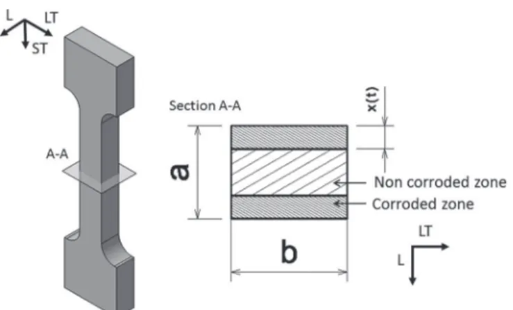
σfail, remained constant for a given metallurgical state of the material. Therefore, the authors proposed to calculate the thickness of the cor-roded, i.e. non-bearing, zone (Figure6), named x(t), where t is the time of immersion in chloride solution before the tensile test, using
the following equation: x(t ) = a 2 µ 1 − Lf ail(t ) Lf ail ¶ [1] where a is the initial thickness of the tensile specimen, Lfail is the maximum load to failure of a non-corroded tensile specimen, and Lfail(t) is the maximum load to failure measured for a tensile specimen pre-corroded for time t.
As said previously, in their work, Augustin et al.17,18used tensile
specimen (Figure1) with a thickness, called a, equal to 1.5 mm. In the present work, to optimize the geometry of the tensile specimens, the same tensile specimens as those used by Augustin et al. were tested but their thicknesses, a, varied from 1.2 to 12 mm (Figure1). In the present work, the tensile specimens were immersed in a 1 M NaCl solution for 24 h to place them under the T2C conditions and to enable comparison with the results obtained by Augustin et al. Corroded specimens were then subjected to tensile testing to evaluate their residual mechanical properties. In this exposure condition, i.e., 24 h continuous immer-sion in a 1 M NaCl solution, Augustin et al. calculated a geometric mean depth for the intergranular corrosion defects of 65 µm (from optical observations of corroded samples), compared with a value of 110 µm for the thickness of the non-bearing zone estimated by the T2C procedure.17 The ST-L faces of the tensile specimens had not been masked from the electrolyte but, the authors ignored in the T2C procedure the corrosion propagation in the LT direction because of the very small surface area exposed in the ST-L plane compared with that exposed in the LT-ST plane. This assumption may not be valid for every tensile specimen (thickness from 1.2 to 12 mm) tested in the present work, and the x(t) value probably over-estimates the real thickness of the non-bearing zone, at least for some tensile specimens. Thus, in the present work, an alternative method based on the T2C procedure was also used to evaluate the thickness of the non-bearing zone. This method, similar to the T2C procedure, calculated the thick-ness of the non-bearing zone assuming that propagation in the LT direction was the same as that in the L direction (this meant that the ST-L plane was not protected from the electrolyte). The thickness of
Figure 6. Schematic of a section of a pre-corroded tensile specimen, with
hatched areas corresponding to the non-bearing zone. The x(t) value varies with time of immersion t. Figure from reference17.
) unless CC License in place (see abstract).
ecsdl.org/site/terms_use
address. Redistribution subject to ECS terms of use (see
195.221.204.225
Figure 7. Schematic of the section of a pre-corroded tensile specimen, with
grey areas corresponding to the non-bearing zone. The d(t) value varies with the time of immersion t.
the non-bearing zone, named d(t), where t is the time of immersion in chloride solution before tensile testing, was calculated using the following equation: d(t ) =1 4 a + b − s (a − b)2+4L(t )f ail Lf ail [2]
where b is the width of the tensile specimen and a, Lfailand Lfail(t) are the same variables used in the T2C procedure as reported in Figure7. As Zhang and Frankel13observed, the propagation in the LT direction
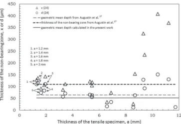
is slower than that in the L direction, thus ensuring that the values of d(t) underestimated the real value of the thickness of the non-bearing zone. However, the calculated x(t) and d(t) values surrounded the real value. Figure8displays the x(t) and d(t) values calculated in the present work for various thicknesses of tensile specimens corroded for 24 h in 1 M NaCl solution. For comparison, the geometric mean depth of intergranular corrosion defects measured, in the present work, from optical observations of corroded samples (52 µm, TableIII) is indi-cated. Furthermore, the data from Augustin’s work,17i.e. geometric
mean depth measured by optical microscopy for the corrosion defects (65 µm) and the thickness estimated by the T2C procedure for the non-bearing zone (x(t) value equal to 110 µm from Equation1) for samples after 24 h of continuous immersion, are also given.
For tensile specimen thicknesses below 1.5 mm, x(t) values were higher than both values from Augustin et al. (estimated thickness of the non-bearing zone and geometric mean depth) and the geometric mean depth measured in the present work despite the fact that negli-gible propagation of the corrosion was observed in the LT direction for these tensile specimen thicknesses. The d(t) values for these tests
Figure 8. Comparison between the thickness of the non-bearing zone (x(24)
and d(24) values) for various thicknesses of tensile specimens pre-corroded for 24 h in a 1 M NaCl solution. Mean geometric depth of the intergranular corrosion defects calculated in this work is reported for comparison as well as results from Augustin et al.17,18
were approximately equal to the geometric mean depth estimated by Augustin et al., but as noted previously, d(t) is assumed to underes-timate the real values. This lack of agreement between the thickness of the non-bearing zone determined by tensile testing compared with the geometric mean depth determined by optical observation can be understood by considering that when taking the 700 µm grain size of the material in the L direction into account, no more than two grains lay in the thickness of the tensile specimen. As a result, an excessively thin tensile specimen would be too sensitive to deep defects, meaning that notch effects would also have to be considered and then the tensile specimen would have to be considered a damaged structural element rather than a homogeneously strained sample. Moreover, considering the results obtained during the CR test and especially the mean and maximal depths of the observed intergranular corrosion defects, for an initial tensile specimen thickness below 1.5 mm, the remaining bearing zone would be too thin, meaning that the results would be too sensitive to the deepest defect rather than to the mean depth of the intergranular corrosion defects. This result showed that the thickness of the tensile specimens had to be adapted to the ratio between the grain size of the specimens and the thickness of the non-bearing zone in order to get a mechanical response characteristic of a polycrystal. However, when dealing with the shape of the intergranular corrosion defects, one had to consider that these defects were not very extended in the LT direction and therefore, the notch effect was not significant except in the case of very thin specimens, i.e. thinner than 1.5 mm.
For tensile specimen thicknesses in the range of 1.5 mm to 5.5 mm, the geometric mean depths of the intergranular corrosion defects were close to the estimated thickness values for the non-bearing zone. This was mainly true for the d(t) values because, with this tensile specimen thickness, it was better to consider the propagation of the corrosion defects both in the L and in the LT directions. The results suggested that the geometry of these tensile specimens was suitable for the T2C procedure by using the d(t) values if the ST-L plane was not protected by a varnish.
Tensile specimen thicknesses over 6 mm resulted in non-acceptable values. Between tensile specimen thicknesses of 6 and 9 mm, both the x(t) and d(t) values were too low, underestimating the real geometric mean depth of intergranular corrosion defects. This can be explained by the fact that under the corrosion condition studied here, i.e., 24 h of continuous immersion, the geometric mean depth of intergranular corrosion was approximately 52 µm, representing a decrease in the mechanical load bearing zone of only 2% for a 6 mm thick tensile specimen and 1.3% for a 9 mm specimen. This reduction in the bearing zone is too small to be detected by the tensile test. For tensile specimen thicknesses greater than 9 mm, the results were not representative as the x(t) values were much higher than the geometric mean depth observed by both Augustin et al.17 and those of the present work.
Moreover, for the thicker tensile specimens, the estimated x(t) value was negative, which is a non-realistic value.
In addition, for all tests, the error in the values estimated from equation1was calculated as follows:
1x = ¯ ¯ ¯ ¯ 1 2 µ 1 −L(t )f ail Lf ail ¶¯ ¯ ¯ ¯1a + ¯ ¯ ¯ a 2Lf ail ¯ ¯ ¯ 1L(t )f ail + ¯ ¯ ¯ ¯ ¯ a L(t )f ail 2L2 f ail ¯ ¯ ¯ ¯ ¯ 1L(t)f ail [3]
The results showed that the error was less than 10 µm for tensile specimen thicknesses below 1.5 mm and approximately 30 µm for thicknesses of approximately 3 mm. The error reached 80 µm for thicknesses of up to 5 mm and was greater than 100 µm for thicker specimens. These data indicate that tensile specimen thicknesses in the range of 1.5 to 3 mm seemed to be the most suitable for the evaluation of the intergranular corrosion defect depth by assessing the decrease in the mechanical properties.
To explain and confirm the fact that tensile specimen thicknesses in the range of 1.5 to 5.5 mm are suitable, a rough calculation was performed. First, all tensile tests were assumed to be reproducible as
the differences in the measured mechanical properties and particularly in the ultimate tensile stress between several identical tests do not vary by more than 10 MPa. Thus, to ensure that a measured decrease in the load to failure is due to the growth of a non-bearing zone rather than due to a lack of accuracy for the load cell, the difference in apparent maximal stress between a non-corroded and a pre-corroded tensile specimen (1σ) must be greater than 10 MPa. Keeping the same notation as in equation1, the problem was formulated as follows:
2x(t )Lf ail=a¡ Lf ail−Lf ail(t )
¢ [4] 2x(t )Lf ail a2b = Lf ail ab − Lf ail(t ) ab [5]
where Lfail/ab = σfailis the ultimate tensile stress of a non-corroded sample and Lfail(t)/ab = σfail(t) is the apparent ultimate tensile stress of a corroded sample. Thus, the decrease in apparent ultimate tensile stress can be written as:
1σ = 2x(t )σf ail
a > 10M Pa [6]
Thus:
a <2x(t )σf ail
10M Pa [7]
The characterization of the corrosion induced by cyclic corrosion tests showed that the non-bearing zone must be at least 50 µm thick to be detected. As previously mentioned, eight non-corroded tensile specimens were tested to determine the reference mechanical prop-erties, yielding an estimated σfailof the uncorroded material of 450 MPa. Taking these data into account, the maximal thickness of the tensile specimens must be 4.5 mm to provide a relevant value for the thickness of the non-bearing zone. These results are similar to those deduced from the data presented in Figure8. However, tensile tests revealed good results for thicknesses close to 5.5 mm. This difference is not surprising given that the decrease in ultimate tensile stress with a non-bearing zone of 50 µm and a tensile specimen thickness of 5.5 mm was approximately 8 MPa, close to the 10 MPa difference estimated previously.
To conclude, these results indicated that to obtain relevant results, tensile specimens tested by the T2C procedure had to be in the range of 1.5 to 4.5 mm thick. In the following part of the present study, the thickness of the tensile specimens was fixed at 2 mm. With 2 mm-thick tensile specimens, it seemed more appropriate to use the d(t) values if the ST-L plane of the specimens were not protected with a varnish to take into account the propagation of the intergranular corrosion defects in the LT direction. However, in the following, for all tensile specimens submitted to a cyclic corrosion test before tensile testing, the surfaces in the ST-L direction were protected with a varnish to consider only the propagation of the corrosion defects in the L direction. Thus, the decrease in the bearing area was essentially related to the propagation of intergranular corrosion on the large sides of the section, i.e. in the L direction. Therefore, the x(t) value was used to estimate the thickness of the non-bearing zone.
Applicability of the T2C procedure to cyclic corrosion tests.—
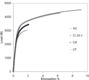
Fig-ure9presents the results of tensile tests for a non-corroded sample (NC) and corroded specimens CR and CF. For comparison with the results obtained for continuous immersion tests, the load/elongation curve of a pre-corroded CI 24 h specimen is also presented. As ex-pected, the mechanical properties decreased for all the corrosion tests compared to a non corroded sample. Furthermore, for both the CI 24 h and the CR samples, the global shape of the tensile curve remained unchanged compared with the curve for the non-corroded specimen, with a homothetic shift in the flow stress. With this result, it could be assumed that the corrosion damage was statistically distributed along the gauge length and that the corroded zone could be considered a non-load bearing zone. This result was less convincing for the CF sample for which the plastic domain was very short; however, ob-viously, a significant shift in flow stress was observed for both CR
Figure 9. Load/elongation curves for non-corroded (NC), CI 24 h (24 hrs),
CR and CF samples.
and CF samples compared to CI 24 h sample with the greatest effect observed for the CF samples despite a lower geometric mean depth for the intergranular corrosion defects for CF samples compared to CI 24 h and CR samples (TableIII). Furthermore, a significant decrease of the elongation to failure was observed for both CR and CF sam-ples compared to non-corroded and CI 24 h samsam-ples. Based on these tests, the thickness of the non-bearing zones was estimated by the T2C method for both CR and CF samples (TableIV). As said previously, because the ST-L plane was protected by a varnish, the x(t) value was calculated. As assumed from the load/elongation to failure curves, the thickness of the non-bearing zone for the CF test was higher than that estimated for the CR test. Furthermore, for both CF and CR tests, the thickness of the non-bearing zone was very different from both the geometric and arithmetic mean depth calculated from optical obser-vations of the intergranular corrosion defects. For the CR test, the x(t) value was three times higher than the geometric mean depth, and for the CF test, the ratio between the x(t) value and the geometric mean depth was about ten. It was also observed that even though the arith-metic mean depths calculated for the CR and CF tests were higher than the geometric mean depths, the results of the T2C procedure were not in agreement with the arithmetic mean depths either. These results indicated that the T2C procedure was not suitable for the estimation of the mean depth of intergranular corrosion defects during cyclic corrosion tests, as all results over-estimated the real mean depth of the intergranular corrosion defects.
Because the defects observed after cyclic corrosion tests exhibited a more branched morphology that those developed during continuous immersion, deeper defects were assumed to have a greater impact on the decrease in the mechanical properties than those formed dur-ing continuous immersion tests, which could contribute to explain the differences between the thickness of the non-bearing zone from
Table IV. Comparison of the estimated thickness of the non-bearing zone from T2C procedure, geometric and arithmetic mean
depths from optical observations of the intergranular corrosion defects for CR and CF samples.
Corrosion test CR CF
x(t) (µm) 217 308
Geometric mean depth (µm) 72 32
Figure 10. The rupture surfaces of tensile specimens pre-corroded under (a)
CR and (b) CF tests. The black area corresponds to brittle surface rupture.
T2C procedure and the real mean depths of the intergranular corro-sion defects. Thus, the rupture surfaces of the pre-corroded tensile specimens were observed by SEM to evaluate the proportion of in-tergranular fractures induced by the corrosion defects. The fracture mode of non-corroded tensile specimens is entirely ductile, whereas zones affected by intergranular corrosion present a brittle mode of rupture. Figure10presents rupture surfaces of tensile specimens pre-corroded under CR (Figure10a) and CF (Figure10b) tests with brittle areas colored in black. Figure10ashows several large brittle zones along the width of the tensile specimen. These areas were sometimes deeper than the deepest defects measured by optical microscopy. This can be explained by the fact that it is likely that the deepest defect was not observed on one of the four analyzed cross sections. Figure
5shows that the analysis of 400 grain boundaries was enough to cal-culate a mean depth for the intergranular corrosion defects but it was probably not enough to evaluate their maximal depth. In Figure10b, for CF pre-corroded tensile specimens, brittle areas were very deep, up to 900 µm, and large proportions of the surface rupture were af-fected by intergranular fracture. This observation was consistent with the high ratio of intergranular corrosion defects observed (TableIII). The proportion of brittle fracture on rupture surfaces was assumed to correspond to the mechanically non-bearing zone, and therefore to allow the measurements of the mean depth of intergranular corrosion defects in a different way. Therefore, fracture surfaces were analyzed closely, and the extent of brittle areas was identified and calculated. An equivalent mean depth named x(t)Swas calculated for comparison to the data obtained by both optical observations of the intergranular corrosion defects and the thickness of the non-bearing zone from the T2C procedure. The values of x(t)Swere calculated using the follow-ing equation where SBis the brittle area observed and b is the width of the tensile specimen.
x(t )S=
SB
2b [8]
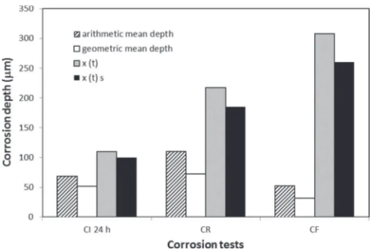
Figure11presents the results obtained for CI 24 h, CR and CF samples. Results showed that calculations of the mean depths of the intergranular corrosion defects from surface rupture observations did not show consistent results for CR and CF tensile specimens even though these values were lower than the values estimated for the thickness of the non-bearing zone using the T2C method.
For CR tests, the ratio of corroded grain boundaries was relatively high, 36%. Almost 15% of the intergranular corrosion defects were deeper than 200 µm and all of the defects were branched, leading to a spreading of the corrosion affected zone. Indeed, independent of the corrosion tests, the anodic reaction corresponded to aluminum
oxi-Figure 11. Comparison of different methods of determining the intergranular
corrosion defect depth for CI 24 h, CR and CF tests. Arithmetic and geometric mean depths are data from optical observations of corroded samples. x(t) and x(t)Sare estimated values from the T2C procedure and from the observation of rupture surfaces respectively.
dation, and, for a short immersion time, the cathodic reactions most likely corresponded to oxygen reduction on the alloy surface and, when the intergranular corrosion propagated, due to the local acidi-fication at the tip of the corrosion defect, to H+
reduction inside the corrosion defect. However, oxygen reduction on the walls of the corro-sion defects was also a possibility. After a long immercorro-sion time, some deep corrosion defects were observed, with the accumulation of cor-rosion products inside these defects and on the surface of the sample. These defects could be rapidly considered an occluded zone charac-terized by a chloride-enriched electrolyte and by H+
reduction as the major cathodic reaction. For CR tests, partial evaporation of the elec-trolyte during the emersion period at room temperature led rapidly to a very high chloride concentration inside the intergranular corrosion defects. This promoted their propagation based on an autocatalytic process since the more the aluminum ions were produced, the more the chloride ions penetrated into the corrosion defects generating a more aggressive solution. However, the corrosion rate was limited by the oxygen reduction kinetics due to oxygen transport to the sample sur-face where the reaction took place. Corrosion products accumulated inside the corrosion defects so that there was rapidly little connection between the tip of the corrosion defects and the external electrolyte.16
Therefore, during the air exposure periods and, for deep corrosion defects during the immersion period, the main reaction was H+
re-duction inside the corrosion defects and the propagation rate of the corrosion defects mainly depended on local chemical conditions.5,16In
this case, there was no limitation by H+
transport processes, which led to extensive propagation of nearly all the corrosion defects compared with continuous immersion tests (TableIII). Furthermore, due to the high chloride concentration inside the corrosion defects, new inter-granular corrosion defects initiated leading to a high ratio of corroded grain boundaries. Because of the high amount of hydrogen produced during corrosion processes, a corrosion-induced hydrogen embrittle-ment could be expected for CR samples as suggested by Kamoutsi et al.11,12 Larignon et al.19,20performed hydrogen content
measure-ments by using a Horiba EMGA-621W and a Br¨uker Galileo HMat Instrumental Gas Analyzers (IGA). They showed that the hydrogen content was 8 ppm, 11 ppm and 25 ppm for non-corroded, CI 24 h and CR samples respectively. The result showed that hydrogen could penetrate inside the corroded material and mainly for the CR sam-ples, in agreement with the kinetics of the corrosion processes, but the amount of hydrogen trapped inside the material was limited because only diffusion processes at room temperature could occur to explain the hydrogen ingress inside the material for CR samples. On the con-trary, for CF samples, the electrochemical processes were limited due the emersion period at negative temperatures leading to mean depth
for the intergranular corrosion defects lower than for CR samples and even CI 24 h samples. However, due to their volume expansion during the emersion period at negative temperatures, the electrolyte and/or the corrosion products trapped inside the corrosion defects gener-ated mechanical stresses strong enough to create a strain state at the tip of the intergranular corrosion defect that could promote hydrogen transport.19,20Hydrogen/dislocations interactions were studied by
dif-ferent authors. For example, Zohdi and Meletis showed that, in the presence of a crack, hydrogen penetration in front of the crack tip can occur mainly by stress assisted diffusion and dislocation transport.24
It was assumed that, for CF tests, this phenomenon was added to a classical hydrogen diffusion process which could occur only during the immersion period at room temperature since the hydrogen diffu-sion coefficient was very low at −20◦
C. Larignon et al. measured a hydrogen content between 50 and 90 ppm for CF samples which cor-roborated this assumption.19,20Further work performed by the same
authors provided evidence of the presence of hydrogen inside the CF samples.21–23
Taking all of these data into account, the applicability of the T2C procedure to cyclic corrosion tests can be discussed. Kamoutsi et al., who provided clear evidence of corrosion-induced hydrogen embrit-tlement in aluminum alloy 2024,11,12 showed that, to consider the
possible effect of hydrogen embrittlement as a volume effect, the cor-rosion layer should have been removed on the tensile specimens and then tensile specimens be constructed to differentiate the effect of corrosion from the effect of hydrogen on ductility. However, for the CR tests, due to the hydrogen content, it was assumed that hydro-gen embrittlement could contribute to the mechanical response of the corroded sample but was not the major phenomenon; the discrepancy between the mean depth of the intergranular corrosion defects mea-sured by optical microscopy and the thickness of the non-bearing zone from the T2C procedure was mainly attributed to the size of the inter-granular corrosion defects themselves. For CR tests, defects appeared on both sides of the tensile specimen, with deep defects observed face to face as in Figure10a, resulting in a significant reduction in the local bearing zone and a large decrease in the mechanical properties. Thus, it could be assumed that the branched intergranular corrosion defects induced a mechanical degradation which was not only related to their mean depth but also to interactions between them. Consequently, the T2C procedure was not an appropriate method to evaluate the mean depth of intergranular corrosion defects following CR tests. However, 90% of the intergranular corrosion defects observed penetrated less than 220 µm, close to the thickness of the non-bearing zone esti-mated by the T2C procedure (217 µm). Therefore, for the CR test, the results of the T2C procedure were more closely related to the maximal depth of the majority of the intergranular corrosion defects than to the mean depth of all defects. Moreover, the few very deep defects, i.e., those deeper than 250 µm, do not have a significant in-fluence on the decrease in the mechanical properties as Augustin et al. suggested.17
For CF tests, the large proportion of very short defects led to a low mean depth of the intergranular corrosion defects compared to the estimation of the non-bearing zone thickness from the T2C procedure. In addition, neither the T2C procedure nor the study of the rupture surface resulted in agreement with the mean depths of intergranular corrosion defects from optical observations. Previous results about hydrogen embrittlement19–23led to the assumption that, for CF tests,
the T2C procedure did not allow estimation of the propagation kinet-ics (mean depth or maximal depth) of intergranular corrosion defects because the decrease of the mechanical properties took into account both intergranular corrosion propagation, which is visible by optical observation, and a hydrogen affected zone that cannot be seen under the microscope. Furthermore, the large proportion of brittle fracture on the rupture surfaces could be attributed to corrosion-induced hydro-gen embrittlement. For CF tests, the T2C procedure seemed to provide an estimation of the damaged thickness of the tensile specimens in-cluding the maximal depth of the intergranular corrosion defects and hydrogen affected area. Thus, the T2C procedure could be a good method to estimate the damage thickness to take into account for
gauging calculations during the design of structural parts. However, as suggested by Kamoutsi et al.,11,12to differentiate the effect of the
corrosion defects from that of hydrogen embrittlement, heat-treatment should be applied to generate hydrogen desorption but this required evaluation of the effect of the desorption treatment on the mechanical properties of the alloy.
Conclusions
This study examined the applicability of the T2C procedure for cyclic corrosion tests and provides a critical analysis of this method-ology previously proposed to determine the mean depth of the in-tergranular corrosion defects on the basis of continuous immersion tests. The T2C procedure was based on the analysis of the me-chanical behavior of corroded samples compared to non-corroded specimens.
(-) Cyclic corrosion tests were alternate immersion-emersion with emersion periods at room temperature for CR tests and at neg-ative temperatures for CF tests. They generated intergranular corrosion defects more branched than after continuous immer-sion. After CR tests, the intergranular corrosion defects were also deeper than those after continuous immersion while, for CF tests, they were shorter. Differences in morphology were explained by taking into account the electrochemical processes. For both CR and CF tests, the ratio of corroded grain boundaries was higher compared to continuous immersion suggesting that the intergran-ular corrosion defects could be statistically distributed along the gauge length of the tensile specimen. Therefore, T2C proce-dure was at first expected to be applicable for cyclic corrosion tests.
(-) The geometry of the tensile specimens used for the T2C proce-dure, i.e. their thickness, was optimized on the basis of intergran-ular corrosion defects developed during continuous immersion tests. Results clearly indicated the major parameter to take into account in such an approach.
(-) The T2C procedure was applied to cyclic corrosion tests. For CR tests, the T2C procedure was assumed to provide a good estimation of the maximal depth of the intergranular corrosion defects. For CF test, this procedure was found to be inadequate due to a hydrogen embrittlement effect. However, it allows cal-culation of the thickness of a corrosion damaged zone including both intergranular corrosion defects and the hydrogen embrittled zone.
References
1. Z. Szklarska-Smialowska,Corros. Sci., 41, 1743 (1999).
2. J. F. Li, Z. Ziqiao, J. Na, and T. Chengyu,Materials Chemistry and Physics, 91, 325 (2005).
3. J. W. J. Silva, A. G. Bustamante, E. N. Codaro, R. Z. Nakazato, and L. R. O. Hein,
Appl. Surf. Sci., 236, 356 (2004).
4. J. R. Galvele and S. M. de Micheli,Corros. Sci., 10, 795 (1970). 5. S. P. Knight, M. Salagaras, and A. R. Trueman,Corros. Sci, 53, 727 (2011). 6. V. Guillaumin and G. Mankowski,Corros. Sci., 41, 421 (1998).
7. M. Posada, L. E. Murr, C. S. Niou, D. Roberson, D. Little, R. Arrowood, and D. George,Mater. Charact., 38, 259 (1997).
8. M. Habashi, E. Bonte, J. Galland, and J. J. Bodu,Corros. Sci., 35, 169 (1993). 9. M. R. Bayoumi,Eng. Fract. Mech, 54, 879 (1996).
10. X. Liu, G. S. Frankel, B. Zoofan, and S. Rokhlin,Corros. Sci., 49, 139 (2007). 11. H. Kamoutsi, G. N. Haidemenopoulos, V. Bontozoglou, and S. Pantelakis,Corros.
Sci., 48, 1209 (2006).
12. H. Kamoutsi, G. N. Haidemenopoulos, V. Bontozoglou, P. V. Petroyiannis, and S. Pantelakis,Corros. Sci., 80, 139 (2014).
13. W. Zhang and G. S. Frankel,Electrochem. Solid-State Lett., 3, 268 (2000). 14. W. Zhang and G. S. Frankel,J. Electrochem. Soc., 149, 510 (2002).
15. W. Zhang, S. Ruan, D. A. Wolfe, and G. S. Frankel., Corros. Sci., 45, 353 (2003).
16. T. Huang and G. S. Frankel,Corros. Sci.49, 858 (2007).
17. C. Augustin, E. Andrieu, C. Blanc, G. Mankowski, and J. Delfosse,J. Electrochem. Soc., 154, C637 (2007).
18. C. Augustin, E. Andrieu, C. Baret-Blanc, J. Delfosse, and G. Odemer,J. Electrochem. Soc., 157, C428 (2010).
19. C. Larignon, J. Alexis, E. Andrieu, C. Baret-Blanc, and G. Odemer,Electrochem Transactions, 33, 39 (2011).
20. C. Larignon, J. Alexis, E. Andrieu, C. Blanc, G. Odemer, and J.-C. Salabura,J. Electrochem. Soc., 158, C284 (2011).
21. C. Larignon, J. Alexis, E. Andrieu, L. Lacroix, G. Odemer, and C. Blanc,Scripta Mater., 68, 479 (2013).
22. C. Larignon, J. Alexis, E. Andrieu, G. Odemer, and C. Blanc,Corros. Sci., 69, 211 (2013).
23. C. Larignon, J. Alexis, E. Andrieu, L. Lacroix, G. Odemer, and C. Blanc,Electrochim. Acta, 110, 484 (2013).
24. T. I. Zohdi and E. I. Meletis, Scripta Metall. Mater. 26, 1615 (1992).