CORRELATION ANALYSIS OF SEDIMENT
DREDGING VOLUMES AND
HYDRO-METEOROLOGICAL VARIABLES IN THE
CORRELATION ANALYSIS OF SEDIMENT DREDGING VOLUMES
AND HYDRO-METEOROLOGICAL VARIABLES IN THE SAINT JOHN
RIVER, NB
By
Sébastien Ouellet-Proulx
Katy Haralampides
André St-Hilaire
Institut national de la recherche scientifique
Centre Eau, Terre et Environnement
(INRS-ETE)
490 De la Couronne, Québec, G1K 9A9
June 2013
TABLE OF CONTENTS
TABLE DES MATIÈRES ... III LISTE DES TABLEAUX ... IV LISTE DES FIGURES ... V
1. INTRODUCTION ... 1
2. ORIGINAL MODEL... 2
2.1DATA AND METHOD ... 2
2.2RESULTS ... 2
3. NEW MODEL... 4
3.1DATA ... 4
3.2METHOD ... 5
3.3RESULTS ... 6
4. DISCUSSION AND CONCLUSION ... 11
5. ACKNOWLEDGMENTS ... 12
iv
LISTE OF TABLES
TABLE 1.R2 AND P-VALUES OBTAINED FROM THE ORIGINAL DATASET AND EXTENDED DATASET ... 3
TABLE 2.LIST OF POTENTIAL PREDICTORS ... 4
TABLE 3.PEARSON CORRELATION COEFFICIENT BETWEEN DREDGING VOLUMES AND EXPLANATORY VARIABLES. (ONLY P-VALUE <0.05 ARE SHOWN) ... 8
LISTE OF FIGURES
FIGURE 1.TIMES SERIES OF DREDGING VOLUMES,JUNEQMAX AND PCPNSPRING ... 7
FIGURE 2.EXHAUSTIVE SELECTION OF INPUT PREDICTORS BY THE MAXIMISATION OF THE ADJUSTED R2 ... 9
FIGURE 3.FORWARD-BACKWARD STEPWISE SELECTION OF INPUT PREDICTORS BY THE MAXIMISATION OF THE
ADJUSTED R2... 9
FIGURE 4.BAR PLOT OF THE OBSERVED DREDGING VOLUMES, THE VOLUMES ESTIMATED FROM THE REGRESSION AND THE VOLUMES ESTIMATED FROM THE LOOCV ... 10
1
1.
INTRODUCTION
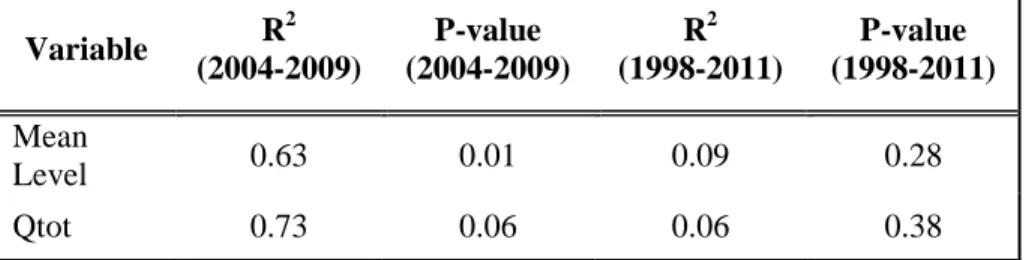
The Saint John Port Authority (SJPA) dredges fine material from the Saint John Harbor, NB every year in order to maintain the required depth for the navigation of large commercial ships. However, the large inter-annual variability in the amount of sediment that they have to dredge induces an uncertainty in the budget allocated for this task. In order to explain a part of that variability, Higgins (2010) tested correlations between hydro-meteorological variables and the volumes of material dredged from the harbor’s bed from 2004 to 2009 using dredging data provided by the SJPA. Significant correlation were found between dredging volumes and mean water level (r2 = 0.63) and total discharge (r2 = 0.73). A multiple linear regression model was built from those variables that explained 83% of the total variance of dredged volumes for those years. Now that additional dredging data have been made available by the SJPA, the work accomplished by Higgins (2010) needs to be re-evaluated. Therefore, the objectives of the present study are to:
1) Verify if the analysis performed by Higgins in 2010 still yield good results
when eight more years of data are added;
2) Investigate if dredging volumes can be linked to other hydro-meteorological
variables;
3) Build a multiple linear regression model using the variables found in
2.
ORIGINAL MODEL
2.1 Data and method
The volume of sediment dredged annually is considered proportional to the sedimentation occurring in the harbor. Therefore, a simple statistical model that could relate hydro-meteorological variables to the volume of sediment dredged would be a valuable tool to estimate the sedimentation in the Saint John Harbor. The model proposed by Higgins (2010) was made from two significantly correlated predictors, mean water level and total discharge of the hydrological year (i.e. October to September). Since then, eight additional years of dredging data were made available by the SJPA (1998 - 2011) for a total of 14 years of data. Therefore, in order to evaluate if the results of Higgins (2010) are still significant when tested on a 14 year time series, the analysis performed by Higgins has been reproduced, with the inclusion of the new data.
Correlation was tested between the predictors used by Higgins (2010; mean water level and total discharge) with additional years and the dredging volumes. A variable was considered significantly correlated when p-value < 0.05.
2.2 Results
When the original model was rerun on a longer time series, the value of the coefficient of determination dropped drastically for both mean water level and total discharge (i.e. the independent variables used in Higgins’ model) and the correlation were no longer significant (Table 1). Therefore, no significant correlation was found for any of the variables considered in Higgins’ work and it was impossible to use the same predictors to build a multiple linear regression model.
3 Table 1. R2 and p-values obtained from the original dataset and extended dataset
Variable R 2 (2004-2009) P-value (2004-2009) R2 (1998-2011) P-value (1998-2011) Mean Level 0.63 0.01 0.09 0.28 Qtot 0.73 0.06 0.06 0.38
3.
NEW MODEL
3.1 Data
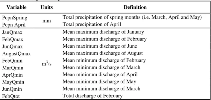
Since reproducing the analysis with the same variables with additional years did not yield any significant correlation, alternative variables were tested. First, the discharge used by Higgins (2010) was estimated using the ratio area method from the discharge recorded by the Water Survey of Canada (WSC) at Grand Falls. For more precision, we used the discharge recorded at the Mactaquac dam which is located about 200 km further downstream.
Table 2. List of potential predictors
Variable Units Definition
PcpnSpring
mm Total precipitation of spring months (i.e. March, April and May)
Pcpn April Total precipitation of April
JanQmax
m3/s
Mean maximum discharge of January
FebQmax Mean maximum discharge of February
JunQmax Mean maximum discharge of June
AugustQmax Mean maximum discharge of August
FebQmin Mean minimum discharge of February
MarQmin Mean minimum discharge of March
AprQmin Mean minimum discharge of April
MayQmin Mean minimum discharge of May
JunQmin Mean minimum discharge of March
FebQtot Total discharge of February
As for the meteorological data, Higgins (2010) used a single meteorological station located in Saint John to account for the whole Saint John River watershed. Since the Grand Falls region is known to be a sediment producing area because of its dense agricultural activity, we hypothesized that sediment transport could be related to precipitation falling in the upper part of the watershed. As an attempt to improve the precision of the estimation of the precipitation data, we used total precipitations interpolated on a 10 km grid, using the ANUSPLIN technique
5
developed by Hutchinson et al. (2009), on the Canadian portion of the watershed (i.e. 64% of the total area). In addition, for both the hydrological and the meteorological variables, correlations were tested on annual, monthly and seasonal data to verify if certain periods of the year could be critical to sediment mobilization.
3.2 Method
From the significantly correlated variable, an exhaustive search was used for the selection of the input variables to build a multiple regression. That method verifies all possible combinations of predictors and selects the combination that returns the best results based on a certain performance criterion (Cornillon and Matzner-Løber, 2006). In this case, the choice was made by
maximising the adjusted R2:
= 1 − − 1
− − 1(1 − )
[1]
Where n is the number of observations, m is the number of predictors included in the model and
R2 is the coefficient of determination, traditionally used to assess model performances. By using
the adjusted R2, in opposition to the standard R2, we ensure that the algorithm takes into account
the number of predictors when choosing the best model and penalise a model that includes more variables.
A stepwise forward-backward regression, which iteratively adds or removes a predictor based on the results of Fisher test, was also tested. This second method was implemented to support the choice of predictors to be included in the multiple regression.
In both cases, a maximum of four predictors was prescribed to avoid overfitting, given the large number of potential predictors and the small sample size. The package leaps of the R software was used to performed the analysis.
To assess the robustness of the multiple linear regression for such a small sample size (14 years), a leave-one-out cross validation (LOOCV) was executed. LOOCV is used to validate model
performances fitted on small datasets. The algorithm iteratively removes the ith observation from dataset to adjust the model and utilizes the resulting model to estimate that observation. When each observation has been estimated, the performance indices can be can be calculated to compare the estimated values to the observed values. In this case, the performance of the model
was verified through the calculation of R2, relative root mean square error (RRMSE) and relative
bias (RBIAS). R2 was used instead of adjusted R2 to assess the performances of the final model
for ease of comparison with similar studies.
Pearson correlation coefficients and their corresponding p-values were calculated to assess the relationship between the volume dredged and the hydro-meteorological variables. A level of significance of 5% was used to determine which variable to include as potential predictors, meaning that only variables with a p-value lower than 0.05 were retained.
For both the variables used by Higgins and the new variables added in this study, we tested annual values calculated for the hydrological year (October to September) instead of the calendar year (January to December) because the dredging usually occurs from July to November (Higgins, 2010).
3.3 Results
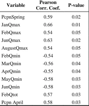
Significant correlations were found for 12 new potential predictors drawn for either interpolated precipitation or discharge at the Mactaquac dam. The significantly correlated variables are listed in Table 3. The highest correlation coefficient was found for January mean maximum discharge (JanQmax; r = 0.66) followed by June mean maximum discharge (JunQmax; r = 0.63) and the total precipitation recorded during springtime (PcpnSpring; r = 0.59). All the other significantly correlated variables have a Pearson correlation coefficient above 0.54 (absolute value).
7 Figure 1. Times series of dredging volumes, JunQmax and PcpnSpring
Table 3. Pearson correlation coefficient between dredging volumes and explanatory variables. (Only p-value < 0.05 are shown)
Variable Pearson
Corr. Coef. P-value
PcpnSpring 0.59 0.02 JanQmax 0.66 0.01 FebQmax 0.54 0.05 JunQmax 0.63 0.02 AugustQmax 0.54 0.05 FebQmin -0.54 0.05 MarQmin -0.56 0.04 AprQmin -0.55 0.04 MayQmin -0.58 0.03 JunQmin -0.58 0.03 FebQtot 0.57 0.03 Pcpn April 0.58 0.03
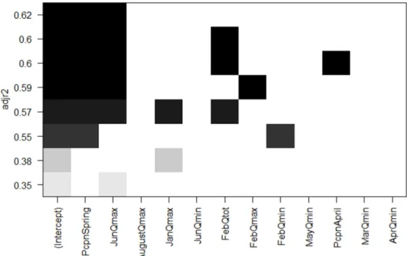
Figures 2 and 3 graphically show which predictors should be used in order to adjust the best possible model on the available data, if respectively an exhaustive search or a stepwise regression is used. Both the exhaustive and the forward-backward stepwise method retained the same predictors to build the multiple regression, namely the total precipitation recorded during springtime (PcpnSpring) and the mean maximum discharge of June (JunQmax; Figures 1 and 2). A linear equation was adjusted using these two predictors by minimizing the sum of the squared error (Equation 1).
= −3177.4 + 69.78 ∗ ! + 1.2 ∗ #$ % &' + ℇ [2]
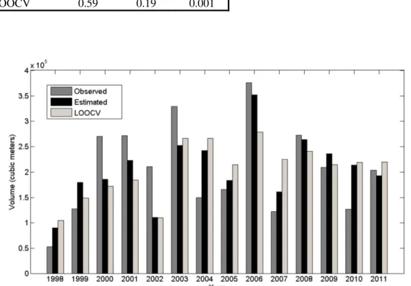
When the regression was fitted on the whole dataset, it returned a R2 of 0.68 while this
coefficient dropped to 0.59 when the LOOCV was implemented. As for the RRMSE, it was 0.16 when the whole dataset was used and it increased to 0.19 for the LOOCV. It both cases, the model was not biased (Table 4). Considering the small sample size, 59% of variance explained on LOOCV data is satisfactory.
9 Figure 2. Exhaustive selection of input predictors by the maximisation of the adjusted R2. The blocks correspond to the predictors of the x axis selected to build a model that would return the adjusted R2 shown on the y axis. The different shades of gray represent the magnitude of the adjusted R2.
Figure 3. Forward-backward stepwise selection of input predictors by the maximisation of the adjusted R2. The blocks correspond to the predictors of the x axis selected to build a
model that would return the adjusted R2 shown on the y axis. The different shades of gray represent the magnitude of the adjusted R2.
Table 4. Performance criteria for the multiple regression and the LOOCV
Method R2 RRMSE RBIAS
Regression 0.68 0.16 0
LOOCV 0.59 0.19 0.001
Figure 4. Bar plot of the observed dredging volumes, the volumes estimated from the regression and the volumes estimated from the LOOCV
11
4.
DISCUSSION AND CONCLUSION
Higgins (2010) stated that the SJPA hypothesised that the volumes dredged annually “should be related to the magnitude of the previous spring flood”. This could not be confirmed by Higgins’ analysis. She suggested that annual total discharge and annual mean water level would be the most appropriate predictors of the dredging volumes according to the available data at the time.
However, the results of the present study seem to support the hypothesis of the SJPA. Among the 12 significantly correlated variables, seven were spring or early summer hydro-meteorological statistics. Also, both the exhaustive and the stepwise selection of predictors obtained highest
adjusted R2 from JunQmax (r = 0.63) and PcpnSpring (r = 0.59) which are spring and early
summer variables. It can be seen on Figure 1 that some years with high dredging volumes (e.g. 2000, 2006 and 2011) correspond to high discharge in June and high spring precipitations. However, such observation should be interpreted with some caution considering that the sample was made of only 14 years of data.
From five other significantly correlated variables, four of them are winter discharge statistics (Table1) and three of these five are from the month of February. Also, for both the exhaustive and the stepwise approaches, if a third predictor was considered in the model, the February total discharge (FebQtot; r = 0.57) was retained (Figures 2 and 3). Although no winter variables were included in the regression built in this study, winter hydro-meteorological should be part of future work. Alternative statistical approaches, such as model trees, or longer time series of dredging volumes may prove that variables characterizing winter conditions to be adequate predictors of the variability in the sedimentation in the Saint John harbor.
5.
ACKNOWLEDGMENTS
The authors acknowledge the contribution of the St. John Port Authority, NSERC and the WATER CREATE program. The authors also wish to acknowledge Agriculture and Agri-Food Canada / Natural Resources Canada (AAFC/RNCan) and Environment Canada
13
6.
REFERENCES
Cornillon P.-A. et Matzner-Løber É.. (2006). "Section 6 : Choix de variables." In: Régression: théorie et applications, Springer-Verlag France, Paris, 143-178.
Higgins H. 2010. Estimation des concentrations de sédiments en suspension dans le fleuve Saint Jean (Nouveau-Brunswick) et établissement de liens avec les données climatiques locales. (Master's thesis). Retrieved from: www1.ete.inrs.ca/pub/theses/T000564.pdf
Hutchinson M, Mckenney DW, Lawrence K, Pedlar JH, 2009: Development and testing of Canada-wide interpolated spatial models of daily minimum–maximum temperature and precipitation for 1961–2003. J. Appl. Meteorol. Climatol. 48:725–741.
Kidd S.D., Curry R.A., Kelly R. Munkittrick. 2011. State of the Saint John River. Canadian Rivers Institute. From: