Discrete element computation : algorithms and architecture

Discrete Element Computation:

Algorithms and Architecture

by

Eric David Perkins

Submitted to the Department of Civil and Environmental Engineering

in partial fulfillment of the requirements for the degree of

Doctor of Philosophy in Information Technology

at the

MASSACHUSETTS INSTITUTE OF TECHNOLOGY

June 2001

©

Massachusetts Institute of Technology 2001. All rights reserved.

A uthor ...

Departi

< off ivil and Environmental Engineering

May 25, 2001

Certified by...

Associate Profes o of Civil and

John R. Williams

Environmental Engineering

Thesis Supervisor

Accepted by ...

_...

ral Buyukozturk

Chairman, Departmental Committee on Graduate Studies

MASSACHUSETTS _INSTITUTE OF TECHNOLOGY

JUN

0 4 2001

Discrete Element Computation:

Algorithms and Architecture

by

Eric David Perkins

Submitted to the Department of Civil and Environmental Engineering on May 25, 2001, in partial fulfillment of the

requirements for the degree of

Doctor of Philosophy in Information Technology

Abstract

The Discrete Element Method is a numerical technique used to model physical phe-nomena through the dynamic interactions of a large number of distinct bodies. The strength of the method lies in its ability to accurately model the behavior of inherently discontinuous media, such as granular, fractured, or powdered materials.

The major computational obstacle in discrete element simulation is the automatic detection of contacts between bodies. For large simulations, the complexity of the con-tact detection process is driven by the general spatial reasoning problem of neighbor searching, in which candidate intersection pairs are selected based on their proximity.

Neighbor search algorithms exist that exhibit linear scaling in the number of bod-ies. These algorithms rely, however, on the assumption of uniformly sized objects. Devaitions from this assuption, inherent in many common physical systems, signifi-cantly degrade performance. This thesis presents a new grid-based algorithm which accomodates objects of varying size.

A new grid-based neighbor search algorithm, called CGrid, is developed to deal with objects of varying sizes. A generic formulation for any number of dimensions is presented. CGrid scales linearly in the number of bodies, and is less sensitive to object size disparity than existing linear algorithms. By combining performance and robustness, CGrid provides a reliable neighbor search solution for general simulation systems.

An architecture for simulation is presented, which is designed to support rapid prototyping and extension development.. The core architecture provides an infras-tructure of generic components for simulation management. The simulation object heirarchy is constructed to address the issues associated with developing extension capabilities, and supporting the wide variety of objects and behaviors which can be employed within the Discrete Element Method.

Thesis Supervisor: John R. Williams

Title: Associate Professor of Civil and Environmental Engineering

Acknowledgments

First and foremost I would like to thank my advisor and committee chair, John Williams. His consistent support, understanding patience, and energetic enthusiasm have been more than I could have asked for. Without him, I am sure I could never have come this far. Thanks also to the other members of my committee, professors Amaratunga and Connor, for their helpful and timely guidance on this thesis and in my studies in general.

To Julia, for taking me in when I needed it, like the family you have always been to me, and for constantly keeping me plied with coffee and good spirits. To Brian and James for putting up with my vagaries, and always being there for advice, and help.

To Ben Cook and Petros Komodromos, thanks for the discussions, without which much of this thesis would be blank. And , of course, thanks for always reminding me of the important deadlines.

Thanks to Joan McCusker for her always amiable help in dealing with MIT, and friendly support and encouragement. I can't imagine what any of us would do without your help.

Lastly, to my parents, my unbending support and unconditional defenders for the past 26 years, you have made this and everything else possible. With love, respect,

Contents

1 Introduction

1.1 The Discrete Element Method . . . . 1.1.1 Contact Penalty . . . . 1.1.2 Geometric Representation . . . . 1.1.3 Contact Detection . . . . 1.2 M IM E S . . . .

I Algorithms

3 Review of Existing Methods

3.0.1 Tree M ethods . . . . 3.0.2 Sorting Algorithms . . . . 3.0.3 Grid-based algorithms . . . . 4 CGrid: Neighbor Searching for Objects with Arbitrary Extents

4.1 SGrid: Generalized Bucketing . . . . 4.1.1 SGrid Contact Mask . . . . 4.1.2 SGrid Subdivision . . . . 4.1.3 SGrid: putting the pieces together . . . . 4.2 CGrid: Supporting Arbitrary Extents . . . . 4.2.1 Discretization of Arbitrary Extents . . . .

4 13 14 14 16 19 20

28

4.2.2 Current and Collector . . . . 4.2.3 The Occupied Bucket Queue: handling sparsity . . . . 4.3 CGrid: Proof of Correctness . . . . 4.4 Implementation Notes . . . . 5 Performance

5.1 Scaling in Simulation Size . . . . 5.2 Sensitivity to Off-Normal Objects . . . . 6 Algorithm Contributions

II Architecture

8.3 8.4

8.2.2 Identifiers . . . . 8.2.3 Cloning . . . . Containers and Lookups . . . . Type Interactions . . . . 8.4.1 Typeld Convention . . . . . 8.4.2 TypeInteractionManager . . 8.4.3 InstanceInteractionManager 9 Simulation 9.1 SimLevel . . . . 9.2 SimLoop . . . . 9.3 Generic SimLoop . 9.4 Modules . . . . 9.5 SimModule . . . . 9.6 SimulationManager 9.7 SimObjManager . . 10 Element

10.1 Goals and Motivation ... 10.1.1 Monolithic Elements 10.1.2 Modular Elements 10.1.3 Shareable Components 10.2 Properties . . . . 10.3 Locale . . . . 10.4 Bounding Box . . . . 10.5 Dynamics . . . . 10.6 Contact . . . . 10.7 Geometry . . . . 10.8 Geometric Intersection . . . . 10.9 M aterial . . . . 10.10Actions . . . . 92 93 95 97 98 99 100 102 102 104 105 106 106 107 108 109 109 109 110 111 111 113 113 114 115 116 117 118 . . . . 119

11 Behaviors

12 Scripted Interface 123

12.1 General Command Guidelines . . . . 123

12.1.1 Option Notation . . . . 124

12.1.2 Help . . . . 124

12.2 Command Infrastructure . . . . 125

12.2.1 CommandLine . . . . 125

12.2.2 Three Phase Evaluation . . . . 126

12.3 ArgStack . . . . 127

12.3.1 PipeLine . . . . 128

12.3.2 PipeDest and PipeSource . . . . 128

12.3.3 Pipes . . . . 129 12.3.4 Pipers . . . . 134 12.3.5 Implemented Pipes . . . . 138 12.4 Benefits . . . 139 12.5 Potential Issues . . . . 140 13 Arhcitecture: Contributions 142 A CGrid Implementation 143 120

List of Figures

1-1 Discrete Elements . . . . 15

1-2 Granular DEM Example . . . . 16

1-3 Contact Law . . . . 17

1-4 2D MIMES Superquads . . . . 18

1-5 DFR Example . . . . 18

1-6 Contact Detection: Neighbor Searching and Geometric Resolution . . 20

1-7 MIMES User Interface . . . . 21

1-8 MIMES: Unconfined Compression in a Bonded Sample . . . . 23

1-9 MIMES: Particle Mixing in a Rotating Drum . . . . 24

1-10 MIMES: Standing Waves in Particles on a Shaker-Table[98] . . . . 25

1-11 MIMES: Bore-Hole Break-out . . . . 26

1-12 MIMES: Hydraulic Fracturing . . . . 27

2-1 Bounding Volumes . . . . 30

3-1 Quad Tree Example . . . . 34

3-2 R-Tree Example . . . . 34

3-3 DESS Example . . . . 36

3-4 Grid-based Methods . . . . 38

3-5 Bucketing Example . . . . 38

3-6 Bucketing and Sparse Simulations . . . . 39

3-7 Grid-based algorithms: over-reporting . . . . 42

3-8 Effect of object size distributions on NBS grid . . . . 43

. . . . 4 6 4-2 3D extension of the NBS Contact Mask

4-3 SGrid Contact Mask (2D) . . . . 4-4 2D Grid Neighborhood . . . . 4-5 NBS Contact Mask in action...

4-6 SGrid Contact Mask in action . . . .

4-7 NBS Contact Mask in action (2) . . . 4-8 SGrid Contact Mask in action (2) . . 4-9 SGrid Subdivision Stages (simplified) 4-10 Typical Subdivider (simplified) . . . 4-11 SGrid 3D Stages . . . . 4-12 Typical SGrid Subdivider . . . . 4-13 Complete SGrid3D Example... 4-14 SGrid Discretization . . . . 4-15 CGrid2D y Subdivider Membership .

5-1 5-2 5-3 5-4 8-1 8-2 8-3 Test Simulation . . . . Performance vs. Number of Bodies . Performance vs. Cell Factor . . . . . Performance vs. Cell Factor (log-log) Euler Angles . . . .

Quaternions

Listings

Locale . . Region . . . . Dynamics . . . . Contact . . . .... . ContactPenalty . . . . PenaltyBasedContact . . . Geometry . . . . IntersectionPoint . . . . . Material . . . . MaterialInteraction . . . . StandardBehavior . . . . . GroupBehavior (interim) BehaviorManagerEntry GroupBehavior (final) BehaviorManager . . . . . CommandLine . . . . ArgStack . . . . PipeDest . . . . PipeSource . . . . ArgPusher . . . . ArgPasser . . . . ArgPiper . . . . ArgPopper . . . . DoubleArgPopper . . . . . ArgSwapper . . . . Command System Syntax Piper . . . . PiperTI . . . . PiperC . . . . PiperT1C1 . . . . . . . . . 113 . . . . . 114 . . . . . 115 . . . . . 115 . . . . . 116 . . . . . 117 . . . . . 117 . . . . . 118 . . . . . 119 . . . . . 119 . . . . . 120 . . . . . 121 . . . . . 121 . . . . . 122 . . . . . 125 . . . . . 127 . . . . . 128 . . . . . 129 . . . . . 130 . . . . . 130 . . . . . 131 . . . . . 132 . . . . . 132 . . . . . 133 . . . . . 134 . . . . . 135 . . . . . 135 . . . . . 136 . . . . . 136 113

P iperT 2 . . . . Helper Functions . . . . CGridParent . . . . CGridAxis . . . . CGridSubdivider . . . . CGridSubdivider Specialization . . . . CGrid Contact Mask subdivide implementation . . CGrid2D Contact Mask subdivide implementation. C G ridSort . . . . . . . . 137 . . . . 138 . . . . 143 . . . 144 . . . 146 . . . . 150 . . . . 152 . . . . 153 . . . . 154

Chapter 1

Introduction

The Discrete Element Method (DEM) provides a powerful way to model the behavior of physical systems using collections of distinct bodies. The method is able, using large numbers of bodies, to capture behaviors which are not well modeled by methods based on continuum assumptions alone. The method finds applicability in situations where the phenomena of interest are rooted in discontinuity. Thus studies of fracturing in ice sheets [36, 32, 76], beams [47], and rock [33, 34, 49], have all been successfully undertaken with discrete element methods. Of particular interest are problems in granular materials, where the discontinuity of the system is can lead to fundamental inaccuracies in a continuum representation. [78, 75].

The goal of this work is to address some of the inherent difficulties in the com-putational and software-architectural aspects of the method, and to provide a high-performance, extensible framework for state of the art research in DEM applications and methods. This chapter gives an overview of the Discrete Element Method, pro-viding insight into current methods, useful tools, and computational obstacles. Part I covers high-performance contact detection algorithms for Discrete Element compu-tation, presenting a new algorithm that scales linearly in the number of bodies, and is appropriate for simulations with distributions of object sizes. Part II presents an architecture for DEM simulation designed with a special emphasis on extensibility, and clear design.

1.1

The Discrete Element Method

The Discrete Element Method (DEM) denotes a set of numerical modeling techniques which takes as it base assumption the discontinuity between its elements, and whose main emphasis is on the solution of contact between those bodies. In general, a DEM simulation involves a number of interacting bodies which undergo large displacements and rotations. The method has been used with rigid and deformable bodies in contin-uous, discontinuous[27, 95, 94], and fracturing[35, 72, 51] configurations, and supports a wide range of material laws, physical behaviors, and geometries.[57]

The method has evolved from early work in a number of disciplines including physics of particles [9, 45, 44, 37, 38], geomechanics [14, 26, 16, 17, 15, 31], and struc-tural engineering [70, 43, 53]. Its theoretical background is founded in the Finite Element Method [11], and the Finite Difference Method. A full theoretical develop-ment of the method can be found in [57].

1.1.1

Contact Penalty

While the Discrete Element Method has been used in conjunction with continuous models to simulate internal deformation of the bodies, we are concerned with the general DEM concept, and will consider a more basic form in which each body is associated with a fixed geometric extent and an independent position and orientation (see figure 1-1). The boundary deformation is modeled using a contact penalty. In the case of continuous bodies, the penalty function represents a compatibility constraint on the continuity of the aggregate geometry. In the case of discontinuous bodies, on the other hand, this penalty function represents an approximate model of impact-induced boundary deformation in the bodies.

One promising area for application of the Discrete Element Method is the study of granular materials [63, 74, 93]. In this case, the goal is to model the material as an aggregate of primarily discontinuous bodies. The inter-body forces can be seen as modeling the micro-scale deformation properties of the material grains. Figure 1-2 shows the use of rigid elliptical discrete elements to simulate the behavior of a soil

Figure 1-1: Discrete Elements: geometry, position and orientation

sample.

Typically, when modeling discontinuous media such as granular materials, the contact is penalized with a linear elastic restorative force, as well as viscous damping, and a frictional shear force. Figure 1-3 shows a schematic view of the individual element-to element contact model. In order to track the history of the frictional force, the contact penalty is resolved incrementally as follows, where

f"

f,

6f, =k,6u, + k,67i,

6fs = k.6u, + /kso67i

The equations of motion are integrated using an explicit scheme, as the dynamic nature of the applied loads can only defined explicitly.

Figure 1-2: Micro-scale and Macro-scale Views of a Discrete Element Simulation

1.1.2

Geometric Representation

As with internal constitutive relations and contact laws, the Discrete Element Method supports a wide array of geometric representations. These range from simple spheres to arbitrarily complex polyhedral geometries.

The boundary representation, in which the geometry is defined by boundary el-ements (i.e. edges or facets) has been used in several discrete element simulation systems [35, 73]. This method is capable of representing complex geometries, but is inefficient in its most basic form. A naive algorithm requires O(M 2) computations to find the intersection of two bodies with M facets or edges. Better performance can be achieved through indexing strategies. For example, the geometry can be partitioned using a tree structure to achieve 0(M lg M) performance.

Williams and Pentland proposed a superquadric scheme in which element

Figure 1-3: Schematic View of the Contact Law: normal and share relations

tries are defined by a superquadric function [88, 90, 89]. Figure 1-4 shows a collection of two dimensional superquadric elements. This method has the advantage of provid-ing a simple test for point inclusion. That is, the value of the superquadric function, evaluated at the point of interest reveals, in its sign, whether the point is inside (pos-itive) or outside (negative) the body. Thus, if the body surface is sampled with M points, the intersection test can be carried out in O(M) computations. Repeated evaluation of the superquadric function is, however, costly, especially if the number of test points is large (i.e. when the surface sampling is very detailed).

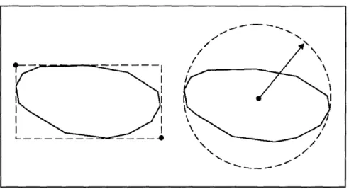
Drawing on the functional representation of the Williams and Pentland scheme, Williams and O'Connor proposed a discrete function representation scheme (DFR) [85, 86, 91, 56, 55]. In this scheme, the discriminant function is defined on a dis-crete grid. The evaluation of the function at a given test point is then reduced to a hashing operation to locate the appropriate grid square, and an interpolation of the corner points to evaluate the function. For a body with M facets, the DFR contact resolution requires O(MI/2) operations. Apart from the performance benefits over the analytical superquadric formulation, the DFR scheme is capable of representing arbitrarily complex bodies, such as the one shown in figure 1-5.

Figure 1-4: Two-Dimensional Superquadric Elements in MIMES

1.1.3

Contact Detection

The DEM simulation software must automatically detect and resolve, at each timestep, all of the contacts between the bodies in the system. This process, called contact detection, is the heart of discrete element simulation, and is also its most computa-tionally intensive proposition. Specific algorithms for contact detection are discussed in part I. Here we simply note the main challenges for contact detection.

The process of contact detection can be divided into two separate algorithms, neighbor searching and geometric resolution (see Figure 1-6). The goal of the neighbor search is to identify and list objects within a certain neighborhood or zone around a target object. The resulting list is often called the neighbor list. The geometric resolution phase compares the target object geometry against the geometry of the objects in the neighbor list in detail. The computational cost of geometric resolution depends only on the complexity of the geometric representation (for example, the DFR scheme of [54, 56] requires O(Mi/2_{) computations if there are M facets in the} geometric representation). The cost of neighbor searching, on the other hand, depends on the total number of objects in the simulation and therefore has the potential for poor scaling; in a naive implementation, where every object is checked against every other object, the cost is O(N2_{) operations. Because the number of objects} treated in discrete element simulation is often large, neighbor searching can become a computational bottleneck. The development of efficient neighbor search algorithms is thus crucial to the overall performance of the simulation.

The separation of neighbor searching from geometric resolution allows the generic problem of finding the intersections of a set of geometric regions to be addressed without reference to the details of local geometry. The separation, which is achieved through the use of simple bounding volumes, ensures that the neighbor search al-gorithm will remain valid for any geometric representation and resolution scheme chosen. Indeed, once separated from the specifics of discrete element geometries and numerical schemes, neighbor searching becomes a general spatial reasoning problem. The solutions to the neighbor search problem advanced in this thesis, therefore, bear

Neighbor Search

Geometric Resolution

* Target t

* Candidate

Figure 1-6: Contact Detection: Neighbor Searching and Geometric Resolution

application to a wide variety of fields including computer graphics and distributed coordination and planning.

The robustness of the neighbor search algorithm to variations in underlying geom-etry is essential in the development of a generalized DEM simulation system, where any number of geometric representations may be used concurrently. The implications of allowing arbitrary geometries to coexist in the system, however, must not be ig-nored. If the neighbor search algorithm is designed with a specific geometry in mind, its performance may degrade when it is used outside that restricted setting [61].

1.2

MIMES

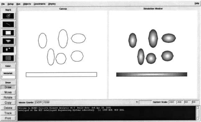
The MIMES project at MIT IESL [63] began as an attempt to bring user-oriented interactivity to discrete element simulation. The combination has proved very suc-cessful, and has fostered significant research in applications as well as algorithms and computational models for DEM. By creating an environment that is interactive and graphical in interface, MIMES allowed users to interact with the simulation in new ways, and to use the tool as an experimental laboratory, for qualitatively investigating multi-body physics. A screen-shot of the MIMES interface is show in figure 1-7.

Prompted by the initial successes of MIMES, and building on the object-oriented design of the MIMES architecture, the project went on to implement a wide vari-ety of extension capabilities, adding functionality to the base environment in new,

0

0

000

Figure 1-7: MIMES User Interface

unplanned ways, leading to many advances in the methods of discrete element simu-lation.

In various versions, MIMES has included support for electrostatic forcing, time varying loads, finite-element fluid forcing, both FEM and BPM internal deformation models, rigid assembly elements, source and sink elements, and four distinct geometric types. While possible in more traditional systems, it is unique interactivity of MIMES that makes it so appealing for experimental development, and an attractive test-bed for new ideas. The ease of use and interactivity has also fostered research in models for contact, bonding, and cloning, and object sources and sinks[60]. Furthermore, the demands of a user-friendly system have prompted research into robust methods for contact detection, resulting in the high-performance algorithm developed in part I.

As a demonstration of the power and generality of such a system, several example simulations are shown in figures 1-8 through 1-12. Figure 1-8 shows an investigation of fracture during unconfined compression in a bonded sample. The elements are bonded using a point-to-point cohesion model, and are being loaded with uniform

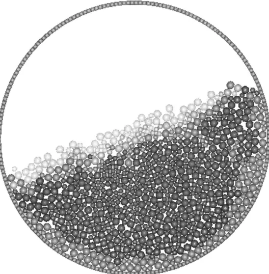
strain. Figure 1-9 shows a simulation of particle mixing in a rotating drum, where the drum is composed of a rigid assembly of quadrilateral elements, and the particles have a distribution of shapes and sizes. Figure 1-10 shows the formation of a standing wave phenomena in a granular assemblage being subjected to vertical vibration through the boundary container [98]. Figure 1-11 shows a simulation of bore-hole break-out, a known fracture phenomena in oil-well bores. Finally, Figure 1-12 shows a simulation of hydraulic fracturing of a well-bore formation, using an extended object source to simulate the fluid loading[20].

The architecture developed in part II is intended to draw from the strengths of the MIMES project, but to avoid some of the pitfalls that were encountered. The most important aspect of the MIMES project to date, in terms of its contribution to discrete element research, has been its use as a test bed for advanced or experimental methods. While the architecture of MIMES proved to be suitable for extension development, it was not initially designed for such dramatic reconfiguration. This has, over the years, led to increase in the complexity of the MIMES core, and necessitated overhaul of some of the core infrastructure. Without a completely new core architecture, however, MIMES extension becomes increasingly difficult. Using a combination of newer technologies, and a design oriented to extension development form the outset, the new DEM Architecture proposes to take the MIMES concept of a computational laboratory even further.

Figure 1-8: MIMES: Unconfined Compression in a Bonded Sample[62]. indicates breakage in the cohesive bonds

Shading r L a NisTt

7M

--..

....

IWO~~

....

a

'Aj

Figure 1-9: MIMES: Particle Mixing in a Rotating Drum. Objects are shaded ac-cording to the magnitude of their velocities

adMkAI

I.

Em'

s-a-I

I

I-IL

-m41

H In

er

Fr

Figure 1-11: MIMES: Bore-Hole Break-out[20]. Objects are shaded to show breakage in the cohesive bonds.

a

I

a

Si

r

U--I

F

F

.1k

_I

a'

m-I

n s a nmfI

StaSh

:;

--I

d

9

ru

-Ad

r

-I

I

F

a1

Figure 1-12: MIMES: Hydraulic Fracturing[20]. Objects are shaded to show breakage in the cohesive bonds.

qI

I

v

p-Fm

Part I

Algorithms

Chapter 2

Neighbor Searching

As outlined in chapter 1, neighbor searching is one of the most computationally intensive parts of a DEM simulation. This is because of the potentially large number of elements involved, and the inherent scaling difficulties of the underlying spatial reasoning problem. This chapter presents an introduction to the problems of neighbor searching. Chapter 3 presents a review of existing neighbor search methods, with some insights into their comparative benefits. In chapter 4, CGrid, a new high performance grid-based algorithm that is designed to support objects with arbitrary extent is developed. Chapter 5 presents the results of performance tests in which CGrid is compared to the NBS algorithm [48].

The interface between local geometry and global neighbor searching is the bound-ing volume (see Figure 2-1). By actbound-ing on the boundbound-ing volume rather than the local geometry, the neighbor search algorithm is able to treat all geometric representations in the same, simplified way. This shifts the focus to the difficult spatial reasoning problem, and makes explicit the notion that the details of local geometry have been suppressed. While any bounding volume could be used, the sphere is the most com-mon, and the one chosen for this implementation. The sphere is represented simply by a position and radius, and is rotationally invariant, so that the extent (radius) need only be computed once for each object for the whole simulation.

The neighbor search algorithm uses the bounding volumes to determine a contact neighbor list (a conservative set of contact candidates) for each object. The complete

Figure 2-1: Bounding Volumes

set of candidate pairs, C determined by the neighbor search algorithm consists of all of the pairs (target, candidate) taken from the contact neighbor lists with duplicate pairings removed. The hypothetical ideal neighbor search algorithm returns a can-didate set Cexact that is exact for the underlying bounding volume in the sense that no pairs are included whose bounding volumes do not overlap. Since the size of the contact neighborhood does not depend on the number of objects, we can say that the size of Cexact is proportional to N.

The obvious goal of neighbor-search algorithm design is to minimize computational costs. In order to achieve better than O(N2) performance, real implementations employ simplifying schemes that quickly identify a conservative approximation to

Cexact. The conservative candidate set C may include candidate pairs whose bounding

volumes do not intersect, but must include every pair whose bounding volumes do intersect. Any such conservative approximation C can be reduced to Cexact by simply applying the exact intersection test for the bounding volume each member, and in practice this step is almost always expedient. For the purpose of analysis, however, the generalized neighbor search algorithm is considered to include no calls to the bounding volume intersection check, and the geometric resolution phase is considered to begin with such a call. This division underscores the compromise, inherent in any neighbor

search algorithm, between minimizing computation time T, and minimizing the size of the candidate set C. These goals are called speed and accuracy, respectively. In most implementations of neighbor searching, and all of the implementations considered here, C is proportional to Cexact (and thus N), but T could scale as poorly as N

squared. This means that for arbitrarily large simulations, speed will be the dominant consideration. Within a finite range of simulation sizes, however, accuracy must also be considered.

As discussed in [61], the underlying geometry and size distribution of the sim-ulation objects may influence the algorithm performance. The algorithm presented here, called CGrid, was developed out previous work [61, 59] on neighbor searching for MIMES. In order to support inexperienced users and to cope transparently with arbitrary simulations, the algorithm is designed to be robust to variations in geometry and object size, and to decouple algorithm performance from rare-case objects.

Chapter 3

Review of Existing Methods

Contact detection, in general, has been long recognized as the major computational obstacle in Discrete Element Simulation [54, 73]. Much of the previous work in the area of contact detection has focused on improved geometric representation and reso-lution algorithms [54, 56, 88, 77, 13], or on integrated neighbor search and geometric resolution schemes [50, 71]. On current scales, where simulations regularly include thousands of objects, N can be considered much larger than M. In this case, the neighbor search algorithm is specifically dominant. Apart from lack of generality, integrated approaches suffer from too much local detail. The increased complexity of resolving the details of contact detract from the algorithm's ability to efficiently address the global-scale problem of neighbor searching.

Body-based methods[57] also figure widely in early references on discrete element computation. In body-based methods, the objects track a body-centered neighbor-hood of nearby objects. This body-centered neighborneighbor-hood is assumed to contain all of the objects which can impact the pivot object in the next few timesteps. In addition to inviting the catastrophic possibility of contact omission, body based methods do not solve the spatial reasoning problem, but rather defer it for longer intervals.

The pressures of the increased simulation size allowed by modern computational resources has led to a shift away from these locally-focused methods of contact detec-tion. Recent schemes have been proposed which better address the principal issues of neighbor searching. These include some tree-based methods, sorting methods, and

grid-based methods. Of these, grid-based methods hold the most promise for future use, since they scale linearly in simulation size.

3.0.1

Tree Methods

Tree-based neighbor search methods index the set of regions represented by the object bounding volumes using a tree structure. The hierarchical nature of tree should be able to provide performance of O(NlgN). Several tree-methods exist, including digital trees, hex trees, k-d trees, and R-trees. Of these, only R-trees are well suited for the representation of regional data (i.e. objects with geometric extent). Other tree methods for intersection tests are typically derived from simpler point-data methods. The extension to regions typically involves an integration of the neighbor search and geometric resolution phases, with the associated problems. Two examples are the tree-portion of the BSD algorithm of Munjiza et al.[50] and the quad-tree implementation of Wensel and Bidanid[71].

In the BSD binary tree, the data points of the underlying polygonal geometric representation are entered individually into a simple BSP (binary space division) tree. The pivot geometry is then used to query the BSP tree starting at the root. This scheme is clearly dependent on the level of detail used in the local geometry, and does not generalize easily to non-polygonal representations. The algorithm performance is best characterized as O(NMlg NM), or O(NM(lgN + g M)), which represents a significant constant multiplier for geometric representations of any complexity.

The quad tree[71] uses a classic quad tree to subdivide space so that leaf nodes either overlap less than two objects, or are sufficiently small. In the case of the suffi-ciently small nodes, the overlapped objects are checked for contact with each other. This algorithm also suffers from entanglement with local geometry. The problem is clear in figure 3-1 where the tree grows inordinately complex trying to decide where, exactly, the two discs overlap.

R-trees are often used for spatial indexing problems in database applications be-cause they are highly general, and well suited to the representation of regional data. In general, an R-Tree is a balanced tree structure in which each node has an

n-I I I

Figure 3-1: Quad Tree Example

dimensional rectangle data value. The rectangle of non-leaf nodes is defined to en-compass the regions occupied by all of the child nodes. In this way, the data rectangles are classified into a tree which is easily queried for data regions intersecting a given query region. Figure 3-2 shows an R-Tree for a small set of rectangles.

~1

Figure 3-2: R-Tree Example

While very general, R-trees are difficult to build. This complexity arises from the freedom allowed in constructing the tree, or more specifically in splitting over-full nodes. Valid trees can be constructed that are highly sub-optimal. It is possible, for

example, to build a valid tree in which all of the non-leaf nodes occupy almost the entire space. In this case, the tree provides worse performance than an exhaustive search. Methods for building well-formed R-trees abound, but all require significant computation (typically quadratic in order) [29, 12, 28]. The objects in a DEM simu-lation are rearranged at each timestep, so the tree must be reformed at each timestep. Since it is not clear how the tree from the previous timestep could be efficiently up-dated, it is essentially necessary to reconstruct the entire tree every timestep. For this reason the R-Tree is not particularly well suited to DEM simulation.

The query performance for the RTree algorithm is difficult to assess since it de-pends on the tree quality. If, however, the tree is well constructed, an individual object query should require O(lg N) operations. Thus the overall query performance, for a well-constructed tree, should be O(Nlg N). If a suitable construction or up-date method were developed, this level of performance could be attractive given the generality of the R-Tree formulation. For truly large simulations, however, the linear performance of grid-based algorithms will always prevail.

3.0.2

Sorting Algorithms

Sorting algorithms attempt to index the set of object-extents by sorting their pro-jections along one or more axes. This approach has the distinct advantage of being straight forward, and adaptable to objects with a distribution of sizes. Unfortunately, the projections do not capture the local intersections well, and so the intermediate candidate sets derived from each axis of projection are large, and grow with increasing numbers of objects. In order to obtain a more accurate candidate set, the intermediate sets must be intersected, and this operation does not scale linearly. Sorting methods derive from point based methods, and early implementations [69] for regional objects were unwieldy. A more recent example of a highly optimized sorting algorithm is DESS.

The DESS algorithm [61] indexes both the upper and lower bounds of each object. The projected upper and lower bounds are sorted in lists for each of the primary spatial axes. The sorted lists are used to determine so-called projection candidates

Figure 3-3: DESS: Intersection of intermediary candidate lists

for each object. The sort and rank procedure can be performed in (nearly) linear time, with limiting assumptions, but the intersection of the projection candidate lists requires O(N2_/3_{) operations because the lists are unordered, so their intersection must}

be found exhaustively. This is shown graphically in figure 3-3, where the shaded area represents the area of object extremities contained in each of the projection candidate

lists for the central pivot object.

Despite the inherent drawbacks of sorting-based algorithms, DESS performs well for moderately sized simulations. For such simulations DESS is comparable to, or outperforms high performance, linear algorithms[61]. It also has the distinct advan-tage of being insensitive to object size. These factors have made it the method of choice in the MIMES project. For large simulations, the scaling costs outweigh the constant order benefits, and a grid-based algorithm is reccomended.

3.0.3

Grid-based algorithms

Grid-based (also called hashing or bucketing) algorithms, which have been in use for some time in large simulations, are based on the assumption that each object can be approximated by a bounding sphere superimposed on a grid-like discretization of space. In the following discussion, the term cell is used to refer to the area of space associated with each grid-point. The term row is used to refer to a one-dimensional line of cells. In three-dimensional discussion slice is used to refer to a two-dimensional discrete slice of space. The general term bucket is used to refer to any collection of objects associated with a given grid point along a given axis, regardless of the number of free ordinates along the other axes.

If the grid spacing used is at least as wide as the widest bounding sphere, each object in the simulation can be associated with exactly one grid cell. Only objects associated with adjacent cells can then come into contact, so the fixed spatial rela-tionships of the grid can be used as a surrogate for the transient relarela-tionships among the objects. An example is shown in Figure 3-4. Since the assignment of buckets is a simple rounding procedure that can be achieved in O(N) operations, the grid offers a way to capture the local contact relationships that is both simple and efficient.

The typical algorithm can be summarized as follows: In one pass over the objects, they can be divided into buckets according to their discrete ordinates along a given axis. Each of the lists of objects associated with those buckets can then be divided on another axis. By subdividing the pivot bucket, as well as its neighboring buckets, in each dimension, all of the contacts can be evaluated using a small number of bucket arrays for each dimension. Because each object is only visited a constant number of times, the computational cost of the whole algorithm is O(N). Figure 3-5 shows the assignment of objects into rows along the y axis (represented by the shaded boxes along the left), and subdivision of two adjacent rows into individual cells along the y axis. Note that, following the convention of NBS[48], the objects are subdivided along the y axis first, and then along the x. The contact mask, visible at the center of the figure, is used to identify neighbor cells for the target cell in the target row.

Figure 3-4: The discrete grid is used to resolve the object neighborhood

Figure 3-6: Sparse simulations present problems for naive bucketing

The obvious advantage of grid-based algorithms is the linear scaling in N. The disadvantages of the grid approximation, however, make them somewhat sensitive to the conditions of arbitrary simulations. In a simple implementation, the algorithm visits each bucket in order, even if it is empty. This means that performance depends on the size of the problem domain, and not just the number of objects. This can pose problems in simulations where the domain is inherently sparse, or where it grows with time. Figure 3-6 shows an example with both isolated and regional sparsities. These sorts of sensitivities make the algorithm too difficult and unpredictable for use in arbitrary simulations.

The NBS algorithm [48] overcomes the performance degradation due to sparse simulations through careful bookkeeping, and object-based traversal of the bucket lists. The NBS loop is given in pseudo-code below. Instead of visiting each row in order as is done in the simple bucketing algorithm, NBS uses the (unordered) object

list to traverse the row array. This is done by looping over the object list, identifying the rows associated with each object. If the given row has not yet been visited, it is subdivided into the array of cells. Within each row, the (again, unordered) list of member objects is used to traverse the appropriate cell array. Each bucket (row or cell) has a visited flag, which is used to keep track of whether that bucket has already been processed. Following this procedure assures that all of the occupied buckets are visited, and that only occupied buckets are ever visited.

foreach obj in globalObjectList { iy = discreteY(obj);

yBuckets [ iy] .append(obj);

ybuckets[iy].visted = false;

}

foreach obj in globalObjectList {

iy = discreteY(obj); if (yBuckets[iy]. visited)

continue;

yBuckets [ iy]. visited = true; foreach obj in yBuckets[iy] {

ix = discreteX(obj);

xBuckets [0] [ix].append(obj); xBuckets[0][ix]. visited = false;

}

foreach obj in yBuckets[iy-1] { ix = discreteX(obj);

xBuckets[1][ix].append(obj);

}

foreach obj in yBuckets[iy] {

ix = discreteX(obj);

if (xBuckets [0][ix ]. visited) continue;

xBuckets[0][ix]. visited = true;

foreach obji in xBuckets[O][ix] {

foreach obj2 in xBuckets[O][ix] after obji checkContact(objl ,obj2);

foreach obj2 in xBuckets[O][ix-1] checkContact(obj1,obj2);

foreach obj2 in xBuckets[1][ix+1] checkContact(objlobj2);

foreach obj2 in xBuckets[1][ix] checkContact(objiobj2);

foreach obj2 in xBuckets[1][ix-1] checkContact(obj1,obj2);

}

}

foreach obj in yBuckets[iy] {

ix = discreteX(obj);

if (! xBuckets[0][ix].emptyo) xBuckets[O][ix]. clear(;

}

foreach obj in yBuckets[iy-1] {

ix = discreteX(obj);

if (! xBuckets[1][ixJ.empty() xBuckets[1][ix]. clear(;

}

}

foreach obj in globalObjectList {

iy = discreteY(obj); if (! yBuckets[ix].empty()

yBuckets [ix]. clear(;

}

Another disadvantage of existing grid-based algorithms, which is not addressed in the NBS algorithm, is that the discretization itself is dependent on the maximum ob-ject size. Specifically, smaller obob-jects are treated as if their potential contacts lie in a

Figure 3-7: Grid-based algorithms: over-reporting

grid-centered neighborhood three times as wide as the largest object. This decreases the accuracy of the algorithm, causing a greater degree of over-reporting (see

Fig-ure 3-7). It is especially problematic if, for example, the object sizes are distributed probabilistically (see figure 3-8). In this case, the largest object is essentially an out-lier, with the vast majority of objects being significantly smaller. This would result in widespread over-reporting poor performance. If the performance degradation is signif-icant enough, the algorithm, while continuing to exhibit linear performance, may be outperformed over some range of N by more general but higher order algorithms[61].

An even more dramatic outlier case can come from problem-specification. When compacting a sample of particles between plates, for example, it is likely that the uninformed user will specify the plates as very long rectangular elements, as shown in figure 3-9.(Note that a more expert user could take advantage of the rigid assembly

0

0

0**

2o

O

0

0e

0

0e

W

W

00 9.

Figure 3-8: Effect of object size distributions on NBS grid

feature of MIMES to create a rigid collection of small rectangles that could be used as a single boundary). This will result in outlier objects which are as large as the simulation itself. The NBS grid is virtually useless in such a situation, since the whole simulation will be encompassed in one or two grid-squares. For such a problem, where the out-of-norm object size ratio is dependent on the simulation size, the performance will not be linear, but rather O(N2 ). Note that performance is also super-linear if the object size distribution is strictly defined as probabilistic.

0

Figure 3-9: Simulation with long boundary rectangles

M ~ :W t

*lp 44

Chapter 4

CGrid: Neighbor Searching for

Objects with Arbitrary Extents

Large simulations require efficient scaling, but nonuniform object sizes adversely effect existing grid-based algorithm performance. The situation is particularly difficult in simulations involving distributions of object sizes, and in situations where boundary objects are extremely large (see section 3.0.3). What is needed is a grid-based algo-rithm that permits objects to cover more than one grid-point, effectively decoupling the algorithm performance from such out-of-norm objects. The algorithm developed in this chapter, CGrid, achieves this objective. By decoupling the algorithm from the largest objects, robustness to outliers is increased. Furthermore, by tailoring the grid-spacing to smaller objects, more pervasive over-reporting is significantly reduced, and performance is improved.

4.1

SGrid: Generalized Bucketing

The CGrid algorithm is essentially a generalization of the Bucketing algorithm that supports objects with arbitrary discrete extents. The method is developed by sep-arating the assumption of fixed extents from the subdivision process. To that end a generalized formulation of the contact mask, as well as the subdivision process is first developed while maintaining the assumption of fixed extents. Both the contact

Figure 4-1: NBS Contact Mask

mask and subdivision procedure are presented in a formulation for arbitrary dimen-sion to fully expose the subtleties of the algorithm at all levels. It should be noted that the arbitrary dimension formulation represents a significant development in its own right as only a two dimensional formulation is given in [48], and the extension to three dimensions involves a number of difficulties not represented in two. In the interest of describing the algorithm as a unit, the general Bucketing formulation is first composed into a fixed-extent algorithm called SGrid, which is then extended in section 4.2 to the complete CGrid algorithm.

4.1.1

SGrid Contact Mask

In two dimensions, The contact mask used in NBS (shown in figure 4-1) only covers two grid-spaces in the first subdivision dimension (y by convention). Thus it only references two concurrent rows of objects. Its extension to three dimensions (figure 4-2), however, proves somewhat unwieldy, covering three grid-spaces in the second dimension. Extensions on further dimensions cover three grid-spaces on every axis but the first. This increases memory costs, and introduces unwanted complexity in the inner loop. Furthermore, the mask itself becomes increasingly complex and difficult to implement.

Figure 4-2: 3D extension of the NBS Contact Mask

Figure 4-3: SGrid Contact Mask (2D)

Figure 4-4: 2D Grid Neighborhood

masking the contact for a specific pivot cell, the SGrid mask resolved contact re-lations among the current grid-square and its three lower-adjacent neighbors. A two-dimensional example is shown in figure 4-3. The NBS lookahead check (from the pivot to the lower-right adjacent cell) is simply delayed a step, and performed as a cross check between the two partially current cells immediately adjacent to the cur-rent cell. The same intersections are found using the SGrid mask, but the formulation extends indefinitely without covering more than two grid-spaces in any dimension.

Figure 4-4 shows a representative two-dimensional neighborhood, where the dark object is the pivot, and the eight lighter objects are the neighbors. The situation is, of course, schematic, and both the pivot and neighbor objects might, in a real simulation represent zero, one or several objects. The five positions of the NBS mask required to resolve all eight pairings are shown in figure 4-5. Similarly, the SGrid mask requires four positions, which are given in figure 4-6.

One subtle difference to note between the NBS and SGrid masks is the question of when to apply the mask in the case of unoccupied cells. In NBS, the rule is simple. The mask is applied at every position where the pivot cell is occupied. Because the SGrid mask does not refer to a single pivot cell, the occupied positions of the SGrid mask are defined differently. The mask is applied at every position where any cell that is current on the last axis is occupied. Examples of how the mask applications change for NBS and SGrid when some of the neighbor cells are unoccupied are shown in figures 4-7 and 4-8. Further detail about occupied buckets is given in section 4.2.3.

000 0 00

000 0

000

0

10

0

0O

000

Figure 4-5: Five Positions of the NBS Mask in the Pivot Object's Neighborhood

0

c .

0

0

0

0

00

Figure 4-6: Four Positions of the SGrid Mask in the Pivot Object's Neighborhood

00 O

O

..

...

CflWO0

0O

0

0

0

Figure 4-7: Three Occupied Positions of the NBS Mask in the Pivot Object's Neigh-borhood

j

Figure 4-8: Three Occupied Positions of the borhood

SGrid Mask in the Pivot Object's

Neigh-- Neigh--(

The cross-checks can be easily extended to any dimension by addressing the vari-ous positions of the mask as either current or lower-adjacent with respect to each axis, and cross-checking intersections for positions which are not labeled lower-adjacent on the same axis. Figure 4-3 shows the addressing encoded as a bit-string, with one representing lower-adjacent on each axis, and zero representing current. The general rule then reduces to a bitwise NAND of the two strings. Note also, that the bit-string label also clarifies the definition of an occupied position of the mask; a given position is considered occupied if there is an object in one of the mask buckets with a zero as the most significant bit.

4.1.2

SGrid Subdivision

The NBS subdivision algorithm, as presented in [48] proceeds as follows. In one pass, all of the objects are distributed into buckets corresponding to uniform rows of space in one dimension. Taking a given row, the objects which were assigned to that row are distributed into another array of buckets divided along the second dimension (cells). By maintaining two adjacent subdivided rows at a time, and using a local contact mask as shown in figure 4-1 on each pivot cell, half of the pivot's contact neighborhood is always accessible, and all of the contacts can be determined in one complete pass.

In a more abstract sense, the process involves a series of self-similar subdivision

stages (see figure 4-9). For convenience in the generic definitions, the SGrid and CGrid subdividers are associated with the axes in their numeric order (x, y, z).

Focusing just on the current bucket, without considering the adjacent buckets, the NBS algorithm can be recast in terms of a recursive series of individual subdivision stages. To make the division more concrete, we will consider each stage to be carried out by a separate Subdivider object, which is associated with a given subdivision axis. The process reduces to the simple recursive operation: Some source set of objects is fed into a Subdivider (see figure 4-10). The objects are arranged in an array of buckets corresponding to a discretization of space along the associated axis. The objects in each bucket are fed, in turn, as source objects into the next Subdivider. At the

Figure 4-9: SGrid Subdivision Stages (simplified)

deepest level of recursion, the current bucket is an individual cell in space. The first object source is the global set of simulation objects, and the last object destination is the contact mask.

The adjacent buckets add a minor complication. Noting from the discussion of the mask in section 4.1.1 that only the current and lower-adjacent buckets are needed, the complete formulation can be developed as follows. The first (x) Subdivider behaves as outlined above, forwarding a single set of objects corresponding to one bucket along the first axis. In the second (y) Subdivider, the buckets in the current array are held over for a second run as adjacent buckets, just as, in simple Bucketing, the most recent row is held over to act as the adjacent row. (Note that the object-based bucket-array traversal of NBS prohibits reuse of the adjacent row, and thus must subdivide both current and adjacent rows). At the end of each pass of the second subdivider, the current bucket array is shifted over into the adjacent bucket array, and new objects are accepted in the current array. The second subdivider has, therefore, two sets of objects to forward at each grid-point, one current, and one adjacent. By extension,

subdivision axis

Figure 4-10: Typical Subdivider (simplified)

these two sets are doubled in the third (z) subdivider, with two current arrays getting shifted into lower-adjacent positions at the end of each pass. The four arrays in the third subdivider correspond to the four possible combinations of current and adjacent on the first two axes axis. The recursion continues, doubling the number of arrays at each subdivision stage, until the contact mask is reached. Figure 4-11 shows the SGrid3D subdivision process including adjacent buckets.

As indicated in the discussion above, the contact mask can be seen as a specialized form of subdivider, in which the objects are checked for contact, rather than subdi-vided and forwarded. In this light, the addressing scheme used in section 4.1.1 on the contact mask takes on even clearer significance. The bit strings are used to encode a hierarchical adjacency, with the most significant bit designating current or adjacent in highest subdivider, and the lower-order bits designating adjacency in the lower

4

Figure 4-11: SGrid 3D Stages

subdividers. To reiterate, at the end of a subdivision run, during the array-shift, all of the current arrays on the last axis (the first half of the set of arrays) are shifted into the corresponding adjacent arrays. For convenience, the first half of the set of arrays is referred to simply as the subdivider's current half, and the other arrays as the adjacent half. This concept extends to the mask itself, for which the first half of the mask cells (the ones with zero as the most significant bit) are referred to as the current half.

Figure 4-12 presents, more formally, the complete typical SGrid subdivider, asso-ciated with the s'th axis (starting at 1). At each subdivision stage, the s parallel sets of input objects are subdivided along the appropriate axis. The s sets corresponding to the current subdivision grid-point are forwarded to the next stage, and subdivided into the next subdivider's current half. Before the next subdivider returns from

pro-3D contact cell

4

Figure 4-12: Typical SGrid Subdivider

cessing, it evicts the adjacent half, and shifts the current half into adjacent positions. Control returns to the calling subdivider, which forwards the s corresponding to the new current grid-point. It should be noted here that the object-based bucket traver-sal used in NBS could easily be accommodated in the SGrid formulation; the object list for each bucket in the current half would be have to be traversed, and the vis-ited flag would be associated with the grid-points (and not the individual buckets). For CGrid, however, this is not feasible (see section 4.2.3, so the SGrid formulation presented assumes that the buckets are traversed in order.

4.1.3

SGrid: putting the pieces together

The above discussion can be assembled into a fixed-extent algorithm, called SGrid for Subdivider-Grid. Figure 4-13 presents the stage-wise operation of the 3D SGrid algorithm, showing both the schematic object volumes and the subdivider arrays. In