Adsorption on interstellar analog surfaces : from atoms to organic molecules

(1)

HAL Id: tel-01238850

https://tel.archives-ouvertes.fr/tel-01238850

Submitted on 7 Dec 2015

HAL is a multi-disciplinary open access archive for the deposit and dissemination of sci-entific research documents, whether they are pub-lished or not. The documents may come from teaching and research institutions in France or abroad, or from public or private research centers.

L’archive ouverte pluridisciplinaire HAL, est destinée au dépôt et à la diffusion de documents scientifiques de niveau recherche, publiés ou non, émanant des établissements d’enseignement et de recherche français ou étrangers, des laboratoires publics ou privés.

to organic molecules

Mikhail Doronin

To cite this version:

Mikhail Doronin. Adsorption on interstellar analog surfaces : from atoms to organic molecules. Chem-ical Physics [physics.chem-ph]. Université Pierre et Marie Curie - Paris VI, 2015. English. �NNT : 2015PA066254�. �tel-01238850�

(2)

THÈSE DE DOCTORAT

DE L’UNIVERSITÉ PIERRE ET MARIE CURIE

Spécialité : Physique

École doctorale : “Physique en Île-de-France”

réalisée

au Laboratoire d’Études du Rayonnement et de la Matière en

Astrophysique et Atmosphères

et Laboratoire de Chimie Théorique

présentée par

Mikhail V. DORONIN

pour obtenir le grade de :

DOCTEUR DE L’UNIVERSITÉ PIERRE ET MARIE CURIE

Sujet de la thèse :

Adsorption on Interstellar Analog Surfaces: from Atoms to

Organic Molecules

soutenue le 28 Septembre 2015

devant le jury composé de :

M. Josep-Manel Ricart Pla

Rapporteur

M. Patrice Theulé

Rapporteur

M. Christophe Petit

Examinateur

M. Lionel Amiaud

Examinateur

M

me

_{Valentine Wakelam}

_Examinateur

M. Jean-Hugues Fillion

Directeur de thèse

(3)

(4)

Chapter 1 Introduction

1.1 Astrophysical Context

To date, almost 200 different molecular species have been detected in various regions of the interstellar space [1] and in various objects of the solar system. These molecules range from elementary species (H2, CO, N2, CO2, H2CO) to larger organic species of

up to 13 atoms including carbon chains, organic and even organometallic compounds that could eventually provide initial molecular stones for the formation of “pre-biotic” molecules. With the advent of new ground-based and space telescopes of high sensi-tivity in the visible, infrared and submillimiter wavelengths, the richness and diversity of molecular compounds discovered in various regions of the interstellar medium is increasing dramatically. Especially, the observations with the ALMA and, in the near future, the NOEMA radio-telescopes are beginning to revolutionize the field by provid-ing ultra-high spatial resolution, in particular within star-formprovid-ing regions, promisprovid-ing a tremendous forthcoming insight into this fascinating but still largely unknown inter-stellar chemical world. The rich organic inventory of space reflects the multitude of chemical processes involved, that on the one hand, build up complex organic molecules (COMs) from simpler entities, and on the other hand, break down large molecules, in-jected by stars, into smaller fragments [2].

Over the last 30 years, significant progress in the understanding of formation, evolution and destruction of molecules in molecular clouds has revealed the crucial role of dust grains which act as catalytic sites for molecule formation and explain the presence of species that pure gas phase chemical networks failed to predict [3]. Gas-surface interactions are now considered as playing a major role in the monitoring of molecular diversity in space. In the interstellar medium and in planetary bodies as well, the condensation and desorption of molecules from the surfaces play an essential role in the physics and chemistry of these objects, driving the different stages of their evolution [2].

Interstellar dust grains are submicron-sized particles made of silicates and/or car-bonaceous cores. In cold regions, such as dense molecular clouds, pre-stellar cores and inner part of proto-planetary disks, grains are covered by an icy mantle, mainly composed of water, but also containing many other compounds. The main ice com-ponents (CO₂, CO, CH₃OH, CH₄) are detected in the solid phase by infrared

(9)

troscopy [4, 5]. These ices can be continuously processed by the impact of cosmic rays, UV-X photochemistry and thermal diffusion, providing a rich molecular reservoir and a source of larger species which, after being released into the gas phase, are more fa-vorably detected by sub-millimeter rotational transitions of molecules. It should be noted here that this observation technique is blind to the molecules that remain on the grain.

From a chemical point of view, interstellar grains provide a surface on which atoms and molecules can accrete, meet and react. They also play the role of a third body in the reactions which efficiently dissipates the excess energy energy released in the reactions. It is the case for the formation of molecular hydrogen, the most abundant molecule in space, which can only be thermalized by interaction with the surface of dust grains. As initially suggested by Tielens and Hagen [6], it is now established than many other species (such as H2O, CO2 or CH3OH) have efficient grain-surface

chemical formation routes.

The mobility and the surface residence time of an adsorbate bound to a surface are related to a fundamental parameter: the binding energy or “adsorption energy”. In case of exothermic reactions, the newly formed molecules on the surface can be eventually ejected promptly into the gas phase after formation. The efficiency of this process is partly determined by the ratio between the energy released by the reaction and the adsorption energy of the molecule just formed. Other non-thermal processes as the sputtering by fast particles in shocks or the desorption induced by cosmic rays and/or by UV-X rays (the so called “photo-desorption” phenomenon), are also critically dependent of the adsorption energy. In other environments such as in hot cores or cometary nuclei, ices are heated and the molecular reservoir is released into the gas-phase by thermal desorption. Again, the adsorption energy is a central parameter to describe the phenomenon.

In summary, the adsorption energies appear to be highly crucial, because their values govern the temperature at which the molecules are condensed on the solid state surface or released into the gas phase, and also (for the smaller species) because they drive the surface mobility and impact the subsequent chemistry. Adsorption energies strongly influence the gas-phase and grain-surface reactions simultaneously. Depending on the physical conditions of the various sources (temperature and densities), the desorption energies are key parameters that can explain (or predict) both the gas phase and condensed phase compositions. In such a context, complex astrochemical networks including the coupling between gas-phase and grain-surface synthesis are under fast development [7–10]. As a consequence, the need for quantitative physical-chemical data becomes more and more important. Today, everyone has to be aware that the transition from elementary molecules towards more complex organic systems could only be solved by developing accurate chemical models supported by relevant laboratory data.

1.2 Physisorption versus Chemisorption

Adsorption energy is governed by the interaction potential between the atoms/molecules adsorbates and the solid surface to which they are bound [11–13]. In the present con-text, the solid, or substrate, is either the bare grain surface, valid for “warm“ (> 100 K)

(10)

1.2. PHYSISORPTION VERSUS CHEMISORPTION 3

environments, or the water-rich icy mantles, valid for colder regions (10-100 K).

1.2.1 Physisorption

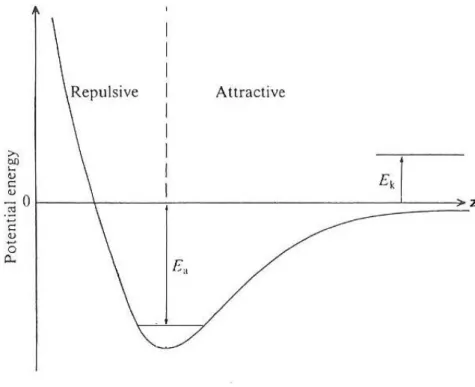
The weakest form of adsorption to a solid surface is called physical adsorption, or physisorption. It is characterized by the lack of a strong chemical bond (covalent or ionic) between adsorbate and substrate. The adsorbed molecule is bound to the surface via weak Van der Waals interactions. The attractive forces are due to a combination of dispersion and dipolar forces. Dispersion forces originate from instantaneous fluc-tuations in electron density, which cause transient dipoles in the molecules. These instantaneous dipole moments interact with the polarizable nearest neighbors on the surface, presenting or not a permanent dipole moment [12]. Forces due to molecules that have permanent dipole moments are usually stronger. In some systems, an hy-drogen atom, bound to an electronegative atom, (NH or OH bonds), is close enough to interact with the lone pairs of another electronegative atom (N/O), leading to the formation of what is called an ”hydrogen bond“. This type of bond is stronger than pure Van der Waals interaction, although weaker than covalent or ionic bonds (see ”chemisorption“ 1.2.2 below). Generally, adsorption on very low temperature surfaces, such as the ones encountered in the interstellar medium, is largely due to physisorption.

Figure 1.1 – Potential energy of an atom or molecule physisorbed on a planar surface.

As illustrated on Figure 1.1, an incoming atom/molecule, with kinetic energy E_k, that losses enough energy when impinging the surface and exciting phonons in the substrate, can equilibrate in a state in the potential well with the binding or adsorption energy E_a. The atom/molecule is said to be accommodated to the surface. Conversely, in order to leave the surface, the atom/molecule must acquire enough energy to escape

(11)

from the depth of the potential well, i.e. Ea. The desorption energy is thus equal

to the adsorption energy. In the case of pure Van der Walls-type of interactions, the adsorption energies for physisorbed molecules are typically ranging between 0.01-0.4 eV. In the case of hydrogen-bonds, the adsorption energies are higher and usually found in the 0.4-0.5 eV range. This will generally correspond to adsorption of organic molecular species playing an important role in astrochemistry.

1.2.2 Chemisorption

In some cases, electron sharing occurs between the adsorbed species and the surface. A rather strong bond is thus created with the surface and the atom/molecule is said to be chemisorbed. The bond formed may be ionic or covalent, or a mixture of both. A simple example of the potential energy diagram for chemisorption is shown in Fig. 1.2. Some of the impinging molecules are accommodated by the surface and become weakly bound in a physisorbed state. Then electronic or vibrational processes can occur, which allows the physisorbed molecules to surmount the barrier Ec and be equilibrated in a much

deeper well. Chemisorption resulting in the formation of a chemical bond between the adsorbing molecule and the surface is at least one order of magnitude stronger (extending from 0.5 to several eV in extreme cases) than physisorption. This process generally results in a profound modification of the local structure like an insertion in the bonds of the surface. It is termed non-dissociative chemisorption. Adsorption can, alternatively, result into the dissociation of the molecule [13], and is then referred to as dissociative chemisorption.

Figure 1.2 – Chemisorption on a planar surface. Adapted from ref [11]

In this work we are concerned only with van der Waals and hydrogen bonding. However, even in this case, we will see that the study of the desorption of atoms and molecules from a grain surface is not as ”simple“ as it may appear.

(12)

1.3. STRATEGIES FOR A RELIABLE DATABASE 5

1.3 Strategies for a reliable database

The lack of basic laboratory data concerning the interaction of many of these molecules on astrophysical relevant surfaces strongly limits the possibilities of the modeling. The adsorption (desorption) energies on surfaces are eventually known for some of the smaller species but mainly assumed (or derived from non-relevant astrophysical stud-ies) for the larger ones. Fundamental laboratory data (experimental and/or theoret-ical) are thus urgently needed to help improving our current understanding of this complex coupled gas-surface chemistry.

This thesis is the first step of a larger project whose main objective is to construct a coherent database that will provide fundamental parameters that can be confidently used to quantify a number of gas-surface interaction processes such as desorption, diffu-sion or trapping of molecules on a dust grain or more generally any kind of interstellar solid. The program is then supposed to be developed around oxygen bearing molecules, nitrogen bearing molecules, large hydrocarbons (PAHs) and finally molecules directly linked to pre-biotic compounds. Aiming at the highest reliability possible, a partic-ular effort had to be been done on the experimental side to optimize a methodology for performing and analyzing experiments based on thermal desorption. Altogether and whenever feasible, the theoretical results produced were confronted with the lab-oratory experiments in conditions as close as possible to the interstellar environment, using well-defined surfaces as prototypes.

Dust grains are thought to be composed of silicates or oxides, surrounded by car-bonaceous materials and/or an icy mantle in some circumstances [5]. The precise composition and morphology of interstellar grains, as well as the identification of the constituents of their icy mantles is of course not fully determined and subject to de-bate. This study deals with different surfaces of various nature and morphology, which could be considered as reasonable interstellar surface analogs: water ice (compact and crystalline) to simulate conditions in cold regions, a graphite surface and a sil-ica monocrystal (chiral quartz) to simulate conditions of warmer carbon/silsil-icate rich regions. The presence and influence of some kind of defects on the surface has also been considered to mimic corrugated carbonaceous solids. Such investigations allow exploring the specificities of these potentially interstellar surfaces, by comparing the behavior of closely related molecules on different surfaces.

The main experimental technique used to study the adsorption/desorption pro-cesses were thermal desorption techniques in the 10-200 K temperature range. These techniques were coupled to Infrared spectroscopy in absorption-reflection mode, well suited to probe surface composition. Such diagnostics have been optimized on the re-cently developed new surface science set-up “Surface Processes and Ices” (SPICES) at LPMAA/LERMA [14, 15]. In particular the recent incorporation of a rotating surface sample holder in the ultra-high vacuum experimental main chamber is well-suited to investigate and compare multiple surfaces under strictly identical conditions. A com-plete description of the experimental set-up is given in part 2.1 and the principle of the data treatment is explained in parts 2.2 and 2.3 on the example of methanol.

When confronting with laboratory experiments, studying the adsorption/desorption processes can be more complex than expected. Practically, two specific situations arise. At first, one can distinguish the so-called “CO-like” species, related to species with

(13)

ad-sorption energies below 0.1 eV. In this case, a single dead-sorption peak appearing at low temperature is observed (typically below 50 K in ultrahigh vacuum conditions) upon thermal heating. That would make the characterization of the desorption energy rel-atively straightforward. However, because the adsorption energy and, by correlation, the diffusion energies, are very low, these extremely weakly bound species are very mo-bile, even at very low temperatures (10 K). This is the case, for example, for CO, H₂, O2 and N2 or atoms physisorbed on water ice. Those species easily diffuse within the

water ice network, being temporally trapped upon heating and giving rise to multiple desorption peaks associated to water ice crystallization and desorption. Another kind of complex situation may occur when the adsorbate-adsorbate interaction energy be-comes significant, that is of the same order of magnitude as mutual interactions within the solid substrate. This is typically the case for organic molecules adsorbed on solid water ice, for which molecule-water, molecule-molecule and water-water interactions can be very similar. It leads to thermal desorption signatures that can be difficult to assign, because it becomes difficult to distinguish between the desorption of the adsor-bate and the water desorption itself. These situations are encountered and discussed in this thesis. For completeness, one should mention that other classifications can be found depending on the desorption behavior of the molecules in ref. [16, 17].

On the theoretical side, the adsorption energy is usually seen as a local property arising from the electronic interaction between a solid support and the molecules de-posited on its surface. The determination of the interaction energy requires the calcu-lation of the energies of the adsorbate molecule, of the pristine surface of the substrate and of the adsorbate-substrate complex, all entities being optimized in isolation.

Two different ways of describing the solid surface can be considered, i.e. the clus-ter model and the periodic model. Representing a grain as a clusclus-ter seems to be a natural approach, but in such a model the surface is that of a molecular aggregate of limited dimension, constrained by the number of molecules participating to the struc-ture. This representation presents several drawbacks. For example, the H2O clusters,

when optimized, present very different surfaces [18] so that there is a complete loss of generality. For larger clusters (over two hundreds molecules), the structure tends to crystalline ice and the calculations becomes rapidly intractable.

Here the theoretical approach has been performed using “state of the art” methods derived from Density Functional Theory (DFT) relying on a periodic description of the solid supports using plane-waves expansions. These methods often referred to as first principle simulations have proved very efficient for both water-ice and carbona-ceous materials [15, 19]. The calculations in the frame of the computational chemistry approach were performed with the Vienna Ab initio Simulation Package (VASP) [20, 21]. The theoretical background of all the methods is presented in the chapter 3.

1.4 Case Studies

The research PhD program has been initiated by an important work on optimizing the method for adsorption energies determination, both experimentally and theoretically. Significant experimental hardware and protocol improvements have been realized, and a method has been proposed for extracting dependable quantitative data from thermal desorption experiments. This latter method has been benchmarked using the study of

(14)

1.4. CASE STUDIES 7

the methanol adsorption on graphite, a case for which some experimental and theoret-ical values were available. A complete and crittheoret-ical analysis of the desorption data for different regimes is presented for this precise case in chapter 2.3. In order to ensure the coupling of the experimental/theoretical approaches, a few specific computational tests have also been performed on this example, though another set of basic tests related to theoretical modeling was carried out on atoms (noble gases) for practical reasons.

The other cases presented here can be referred to as systems of interest for the Titan, the MIS and comets, respectively.

The first issue addressed in this thesis, in which adsorption may play a crucial role, is that of the depletion of argon, krypton and xenon observed in Titan atmosphere. The biggest satellite of Saturn is the only moon of the solar system with a really signif-icant atmosphere. A surprising characteristic of its atmosphere is that no other heavy noble gas than argon has been detected by the Gas Chromatograph Mass Spectrometer (GCMS) on board of the Huygens probe when descending towards the surface of Titan in 2005. Moreover the argon which is detected is essentially 40Ar, which is produced by the radiogenic disintegration of potassium 40K, and some primordial 36Ar, very under-abundant compared to the solar value (about 6 orders of magnitude) [22]. The other primordial noble gases, i.e. 38Ar, krypton and xenon, have not been detected by the instrument GCMS, which implies that their molar fractions are less than 10−8 (detection limit of Huygens GCMS) in Titan atmosphere. This noble gases deficiency has been extensively studied and multiple scenarios proposed but none of them gives a satisfactory global explanation. These scenarios are related either to the internal properties of Titan and the specific structure of its atmosphere or to the formation conditions of Titan in the primitive nebula [23–30]. Among them, Osegovic and Max suggested that the noble gases could have been stocked in ices under clathrates allo-morphs supposed to be present in Titan, and performed some successful exploratory studies with xenon [23]. The hypothesis was then reactivated by Mousis and collabo-rators for Xe, Kr and Ar [24, 25]. This kind of trapping seems to be possible though its efficiency is still to be proved, but in fine it has to be reminded that the existence of such mechanism relies on the mere relevance of forming clathrates in interstellar con-ditions, which is still highly controversial. This is why we turn towards the adsorption trapping by other more conventional forms of ices. The mechanism considered here is the adsorption/inclusion by the dominant solid surfaces available in the primitive nebula, i.e. the compact or crystalline icy grain mantles; those grains being the origi-nal constituents of Titan, this process should have had an impact on the noble gases abundances, which has yet to be investigated.

The second issue addressed, in which adsorption may also be a determining fac-tor, is that of the relative abundances of isomers observed in the gas phase of the interstellar medium (ISM). Here we focus on the CH₃CN and CH₃NC isomers. These compounds are representatives of the nitrogen bearing molecules. They belong to the family of nitriles R-CN and iso-nitriles R-NC which, together, represent about 20% of the observed species. Not only these molecules are key molecules in the evolution chain towards complexity and emergence of species of astrobiological interest, but the abun-dance ratios of their isomers have also been widely used to constrain the astrochemical models. The couple HCN/HNC is well known to present gas phase abundances very sensitive to localization [31, 32], contrary to CH₃CN/CH₃NC whose abundance ratio

(15)

is very steady [33, 34]. Considering that radio astronomy technique cannot detect the molecules depleted on surfaces, that is molecules whose rotation is inhibited, it seems compulsory to take into account the adsorption factor in the determination of abun-dances. As the environment obviously plays a decisive role, we chose to study three different surfaces likely to figure reasonable analogs of interstellar surfaces, with the purpose of covering the panel of surfaces supposedly available in the ISM: water ices, graphite and silica.

The third issue addressed, in which the interaction between an adsorbate and a solid may be critical, is that of the presence of a neutral sodium tail in some comets that are notably composed of water ice accreted onto a refractory nucleus.

Comets are thought to be among the most pristine material in the solar system. Their compositions represent the end point of processing that began in the parent molecular cloud core and continued through the collapse of that core to form the proto-sun and the solar nebula, with the final stages during the evolution of the solar nebula itself as the cometary bodies were accreting. Disentangling the effects of the various epochs on the final composition of a comet is complicated. But learning about the physical and chemical conditions under which comets formed can teach us a lot about the types of dynamical processing that shaped the solar system we see today. This is the objective of the Rosetta mission, which actually boosts all studies about comets.

The observation of comet C/199501 Hale-Bopp in spring 1997 led to the discovery of a new tail connected with the sodium D line emission [35, 36]. Later on, several observations of this phenomenon were recorded in other comets [37, 38]. It means that we are in presence of a neutral sodium gas tail totally different from the usual ion and dust tails, and whose associated source is unclear. Several suggestions have been advanced to rationalize the phenomenon, all physical reasons and unsatisfactory. The shaping of a third type of tail by radiation pressure due to resonance scattering of sodium atoms [35, 38], the photo-sputtering and/or ion sputtering of nonvolatile dust grains [37], or the collisions between the cometary dust and very small grains [39] were considered.

In this thesis, the scenario presented is completely different since it is entirely based upon chemical grounds. It is shown that the Na+ ions washed out of the refractory material at the epoch of the hydration phase of the comet nucleus, are progressively losing their positive charge to evolve into neutral species during the re-formation of the cometary ices. The chemical path of sodium ends with a neutral atom adsorbed at the surface and finally released from the sublimating cometary ice, largely contributing to a pure neutral sodium tail.

(16)

REFERENCES 9

References

[1] Holger S.P. Müller et al. Molecules in Space. www.astro.uni-koeln.de/cdms/molecules, 2015.

[2] A. G. G. M. Tielens. “The molecular universe”. In: Reviews of Modern Physics 85.3 (2013), pp. 1021–1081.

[3] Daren J. Burke and Wendy A. Brown. “Ice in space: surface science investigations of the thermal desorption of model interstellar ices on dust grain analogue sur-faces”. en. In: Physical Chemistry Chemical Physics 12.23 (June 2010), pp. 5947– 5969.

[4] Emmanuel Dartois. “The Ice Survey Opportunity of ISO”. en. In: Space Science

Reviews 119.1-4 (Aug. 2005), pp. 293–310.

[5] A.C. Adwin Boogert, Perry A. Gerakines, and Douglas C.B. Whittet. “Obser-vations of the Icy Universe”. In: Annual Review of Astronomy and Astrophysics 53.1 (2015), null.

[6] A. G. G. M. Tielens and W. Hagen. “Model calculations of the molecular compo-sition of interstellar grain mantles”. In: Astronomy and Astrophysics 114 (1982), pp. 245–260.

[7] R. T. Garrod and E. Herbst. “Formation of methyl formate and other organic species in the warm-up phase of hot molecular cores”. In: Astronomy &

Astro-physics 457.3 (2006), p. 10.

[8] H. M. Cuppen and Eric Herbst. “Simulation of the Formation and Morphology of Ice Mantles on Interstellar Grains”. en. In: The Astrophysical Journal 668.1 (Oct. 2007), p. 294.

[9] George E. Hassel, Eric Herbst, and Robin T. Garrod. “Modeling the Lukewarm Corino Phase: Is L1527 Unique?” en. In: The Astrophysical Journal 681.2 (July 2008), p. 1385.

[10] R. T. Garrod, V. Wakelam, and E. Herbst. “Non-thermal desorption from in-terstellar dust grains via exothermic surface reactions”. In: Astronomy &

Astro-physics 467.3 (2007), p. 13.

[11] M. Prutton. Introduction to Surface Physics. Oxford science publications. Claren-don Press, 1994.

[12] A. Zangwill. Physics at Surfaces. Cambridge University Press, 1988. [13] E.M. McCash. Surface Chemistry. Oxford University Press, 2001.

[14] M. Bertin et al. “Adsorption of Organic Isomers on Water Ice Surfaces: A Study of Acetic Acid and Methyl Formate”. In: The Journal of Physical Chemistry C 115.26 (2011), pp. 12920–12928.

[15] M. Lattelais et al. “Differential adsorption of complex organic molecules isomers at interstellar ice surfaces”. In: Astronomy & Astrophysics 532 (Aug. 2011), A12. [16] Mark P. Collings et al. “A laboratory survey of the thermal desorption of astro-physically relevant molecules”. en. In: Monthly Notices of the Royal Astronomical

(17)

[17] Serena Viti et al. “Evaporation of ices near massive stars: models based on lab-oratory temperature programmed desorption data”. en. In: Monthly Notices of

the Royal Astronomical Society 354.4 (2004), pp. 1141–1145.

[18] Victoria Buch * et al. “Solid water clusters in the size range of tens–thousands of H2O: a combined computational/spectroscopic outlook”. In: International

Re-views in Physical Chemistry 23.3 (2004), pp. 375–433.

[19] M. Lattelais et al. “Differential adsorption of CHON isomers at interstellar grain surfaces”. In: Astronomy & Astrophysics 578 (June 2015), A62.

[20] G. Kresse and J. Hafner. “\textit{Ab initio} molecular dynamics for open-shell transition metals”. In: Physical Review B 48.17 (1993), pp. 13115–13118. [21] G. Kresse and J. Hafner. “\textit{Ab initio} molecular-dynamics simulation of

the liquid-metal\char21{}amorphous-semiconductor transition in germanium”. In: Physical Review B 49.20 (1994), pp. 14251–14269.

[22] H. B. Niemann et al. “The abundances of constituents of Titan’s atmosphere from the GCMS instrument on the Huygens probe”. en. In: Nature 438.7069 (2005), pp. 779–784.

[23] John P. Osegovic and Michael D. Max. “Compound clathrate hydrate on Titan’s surface”. en. In: Journal of Geophysical Research: Planets 110.E8 (2005), E08004. [24] C. Thomas et al. “A theoretical investigation into the trapping of noble gases by clathrates on Titan”. In: Planetary and Space Science. Surfaces and Atmospheres of the Outer Planets, their Satellites and Ring Systems, Part IV Meetings held in 2007: EGU: PS3.0 & PS3.1; IUGG/IAMAS:JMS12 & JMS13; AOGS: PS09 & PS11; EPSC2: AO4 or PM1 56.12 (2008), pp. 1607–1617.

[25] Olivier Mousis et al. “Removal of Titan’s Atmospheric Noble Gases by Their Sequestration in Surface Clathrates”. en. In: The Astrophysical Journal Letters 740.1 (Oct. 2011), p. L9.

[26] D. Cordier et al. “About the Possible Role of Hydrocarbon Lakes in the Origin of Titan’s Noble Gas Atmospheric Depletion”. en. In: The Astrophysical Journal

Letters 721.2 (Oct. 2010), p. L117.

[27] Ronen Jacovi and Akiva Bar-Nun. “Removal of Titan’s noble gases by their trapping in its haze”. In: Icarus 196.1 (2008), pp. 302–304.

[28] Antti Lignell et al. “On theoretical predictions of noble-gas hydrides”. In: The

Journal of Chemical Physics 125.18 (Nov. 2006), p. 184514.

[29] O. Mousis et al. “Sequestration of Noble Gases by H+3 in Protoplanetary Disks and Outer Solar System Composition”. en. In: The Astrophysical Journal 673.1 (Jan. 2008), p. 637.

[30] F. Pauzat et al. “Gas-phase Sequestration of Noble Gases in the Protosolar Neb-ula: Possible Consequences on the Outer Solar System Composition”. en. In: The

Astrophysical Journal 777.1 (Nov. 2013), p. 29.

[31] P. P. Tennekes et al. “HCN and HNC mapping of the protostellar core Chamaeleon-MMS1”. In: Astronomy & Astrophysics 456.3 (2006), p. 7.

(18)

REFERENCES 11

[32] A. Fuente et al. “Observational study of reactive ions and radicals in PDRs”. In:

Astronomy & Astrophysics 406.3 (2003), p. 15.

[33] Anthony J. Remijan et al. “A Survey of Large Molecules toward the Proto-Planetary Nebula CRL 618”. en. In: The Astrophysical Journal 626.1 (June 2005), p. 233.

[34] J. Cernicharo et al. “Tentative detection of CH3NC towards SGR B2”. In:

As-tronomy and Astrophysics 189 (1988), p. L1.

[35] G. Cremonese et al. “Neutral Sodium from Comet Hale-Bopp: A Third Type of Tail”. en. In: The Astrophysical Journal Letters 490.2 (Dec. 1997), p. L199. [36] G. Cremonese et al. “Neutral sodium tails in comets”. In: Advances in Space

Research 29.8 (2002), pp. 1187–1197.

[37] F. Leblanc et al. “Comet McNaught C/2006 P1: observation of the sodium emis-sion by the solar telescope THEMIS”. In: Astronomy & Astrophysics 482.1 (2008), p. 6.

[38] Anita L. Cochran et al. “Spatially Resolved Spectroscopic Observations of Na and K in the Tail of Comet C/2011 L4 (PanSTARRS)”. en. In: AAS/Division

for Planetary Sciences Meeting Abstracts. Vol. 45. Oct. 2013.

[39] W.-H. Ip and L. Jorda. “Can the Sodium Tail of Comet Hale-Bopp Have a Dust-Impact Origin?” en. In: The Astrophysical Journal Letters 496.1 (Mar. 1998), p. L47.

(19)

(20)

Part I

Employed Methods

(21)

(22)

Chapter 2 Experimental approach

This chapter describes all the aspects of experimental study of adsorption of astro-physically relevant species on models of ISM grain surfaces.

First part presents the experimental setup and gives some insights on the prin-cipals of instruments operation. Various experimental issues are discussed, including reproducibility and accuracy.

An introduction to the Temperature Programmed Desorption (TPD) technique is given in the second part.

In the last part the experimental method is described in detail. Data treatment procedure is demonstrated using the example of Methanol (CH₃OH) adsorption on

graphite.

2.1 Experimental setup

SPICES, acronym for Surface Processes and ICES, is an experimental setup developed since 2010 in Laboratoire d’Études du Rayonnement et de la Matière en Astrophysique et Atmosphères (LERMA), Pierre and Marie Curie University, Paris, France. It is an ultrahigh vacuum (UHV) setup intended to study thermal and ultraviolet/VUV photodesorption of species from astrophysically relevant surfaces. Designed as a mobile experiment, it can be transported and coupled to a synchrotron radiation source to study photodesorption. When not coupled to a light source, it can be employed to study thermal desorption.

2.1.1 General description and characteristics

Conditions in the cold regions of the ISM are characterized by extreme low tempera-tures (below 100K) and densities of some hundreds of molecules per cm3, c.f. Chap-ter 1.1 and e.g. [1].

To study the interaction of gases and models of interstellar grains, UHV (2.1.4) and cryogenic temperature (2.1.2) conditions are necessary. Need for ultra-high vacuum comes from the fact that sample surfaces need to be kept clean. Low desorption temperatures of 10-15K for Hydrogen H2, 25-45K for diatomic molecules like CO and

N2, and 100-150K for water and small organic like CH3OH justify the need of cryogenic

temperatures at such low pressures.

(23)

Rotatable 3-faces sample 10K<T<300K UHV chamber P~10-10_Torr ice gr owth system IR MCT_detector FTIR spectrometer --IR-- --IR----VUV --VUV-UV light coupling QMS detector Desorbed species

Figure 2.1 – SPICES UHV chamber instruments

A schematic diagram of SPICES UHV chamber is presented on a figure 2.1. SPICES setup has three sample surfaces: polycrystalline gold, quartz (alpha-0001) and highly-oriented pyrolithic graphite (HOPG), mounted on a sample holder on a tip of the cryocooler cold finger (sect. 2.1.2 a). Temperature of the sample holder and surfaces is controlled within the range of 10 to 300 Kelvin, with 0.01K precision and absolute accuracy of 0.5K (sect. 2.1.2 b). Cryostat assembly is mounted on a rotatable stage, permitting to orient the surface of interest against the dosing line or facing the QMS.

Ices are grown on sample surfaces in situ using a retractable dosing line (see sec-tions 2.1.5, 2.1.6).

To probe the adsorbate in the condensed state a Fourier-Transform Infrared (FTIR) spectrometer is used (namely Bruker Vector 22 with Mercury Cadmium Telluride (MCT) detector), working in reflection-absorption mode.

Desorbed species are detected with a QMS, Pfeiffer Vacuum Prisma 80 with chan-neltron detector (see section 2.1.3 for details).

Pressure in the vacuum chamber is monitored using a Bayard-Alpert gauge, in junction with Varian Multi-Gauge controller. The chamber is pumped with a high-performance turbomolecular pump (Pfeiffer Vacuum HiPace 800), backed by a dry scroll pump (Pfeiffer Vacuum XDS-10). Base pressure stays in a range of 1.5 · 10−10 to 4 · 10−10 mbar, depending on the experiment history.

(24)

2.1. EXPERIMENTAL SETUP 17

2.1.2 Cryogenics and temperature control

To control the substrate temperature in a range of cryogenic temperatures, three ele-ments are necessary: a heat sink (cryocooler, see 2.1.2 a), heat source (electric resistive heater) and a temperature sensor (silicone diode) located as close to the controlled point as possible. Sumitomo CH204 N UHV cryocooler UHV cable feedthrough CF mount ﬂange 1st stage cold end 2nd stage cold end Sample holder Thermal shield Cold ﬁnger extender Compressed He feed Sapphire plate

Figure 2.2 – SPICES cryostat assembly diagram.

A diagram of SPICES cryostat assembly is shown on the figure 2.2. Cryocooler is a commercial Gifford-McMahon type closed-cycle helium type, Sumitomo CH-204 model. A home-made sample holder is attached to the cryocooler cold finger through the oxygen-free high thermal conductivity (OFHC) copper extender. A sapphire (Al2O3)

crystal plate is inserted between the cryocooler extender and the sample holder to reduce the heat transfer when operating at high temperatures (above 70-100K). Cryo-genic part is isolated by a gold-plated OFHC copper thermal shield kept at tempera-tures around 100K to avoid heating by the infrared radiation.

Temperature sensor and heater are located on the sample holder (see the fig. 2.4a, sect. 2.1.2 b). Cryocooler operates constantly at maximum cooling power, while heater output is varied according to PID algorithm (see sect. 2.1.2 b) as a function of tem-perature sensor readings and target temtem-perature.

(25)

2.1.2 a Helium closed cycle cryocooler

With considerably improved reliability and reduced dimensions and costs over last twenty years, cryocoolers became of widespread use for the applications where cryo-genic temperatures are necessary.

Advantage of closed cycle He cryocoolers over open circuit system is reduced opera-tion cost: cryocoolers operate for long periods without or with little maintenance. For example, a maintenance interval of cryocooler used in SPICES setup is 13000 hours, that is a year and a half of constant operation.

The only disadvantage of Gifford-McMahon cryocoolers is the vibration induced by moving parts of the cryostat. Although not an issue for our experiment, it renders impossible the usage of GM cryocoolers in junction with vibration-sensitive surface science methods like STM and AFM microscopy, as well as techniques that need to have the top surface layer in the focal plain (X-ray diffraction).

Vl Vh Compressor water cooling rotary

valve displacer/_regenerator

co ld ﬂ a n g e Ta Cryocooler assembly

Figure 2.3 – Gifford-McMahon cryocooler schematic diagram

A schema of a Gifford-McMahon cryocooler [2] stage is shown on a figure 2.3. It uses compressed helium at room temperature. A working volume may be connected to the high or the low pressure lines of a compressor with help of a rotary valve. Displacer/regenerator piston is actuated synchronously to the valve. Refrigeration cycle consists of four steps:

• Displacer is in the extreme right position, cold volume is minimal. Working volume is connected to the high-pressure line and is filled up to the high pressure. • Displacer moves to the extreme left position, helium is passing through the re-generator to the cold volume and is precooled to the temperature of cold space. • The valve connects the working volume to the low-pressure line, helium is cooled down during the expansion, taking a portion of heat from cold space heat ex-changer and regenerator.

• Displacer moves back to the extreme right position, reducing the volume of the cold part to a minimum. The cycle is closed, the system is back to the state where it was before the first step.

In ideal conditions an amount of heat taken from the cold space is equal (ph− pl)V

where p_h is the helium feed pressure, p_l the return pressure and V the expansion volume in the cryostat cold head.

(26)

Two or three stages may be stacked one after another to reach extreme cold tem-peratures down to 4K. Modern cryocoolers operate with temtem-peratures around 30K on the first stage, 10K on the second stage and down to 4K on the third stage. The lowest attainable temperature on the third stage is limited by helium gas-liquid transition. Use of proper pre-cooled thermal shield is necessary to isolate the cryogenic stage from the infrared radiation.

Physics of cryocoolers is described in a paper of Waele [3], and a general review of current state and progress in cryocoolers development is given by Radebaugh [4]. 2.1.2 b Temperature measurement and control

Temperature of the sample is measured by a silicone diode (calibrated LakeShore DT-670) mounted on a sample holder (see fig. 2.4a). Diode needs to be placed as close to the sample as possible to provide accurate readings. To compensate for cable resistance, a four-wire connection schema is used (fig. 2.4b). Current is fed through one pair, voltage drop on diode junction is measured through another. This approach allows to achieve stable and accurate temperature readings, whatever the length of the cables.

Sample surfaces Temperature sensor Heater capsule Cryostat extender

(a) Spices sample holder

I± V± Heater OUT Temperature controller DT670 Heater R=25 Ω Sensor IN

(b) Heater and temperature sensor connection

Figure 2.4 – Sample holder schema and connection diagram

For the cryogenic part, a twisted phosphor bronze wire is used to limit thermal transfer over the diode leads. Shielded double twisted pair cable is used for connection between the cryostat and the temperature controller.

A resistive cartridge is used as a source of heat. Variable power applied to the heater to maintain the sample temperature is controlled by LakeShore 336 using Proportional-Integral-Derivative (PID) algorithm.

(27)

2.1.2 c PID control

Initially developed in the beginning of 20th century for automatic guidance of transat-lantic ships, PID control principle is widely used nowadays to control parameters of systems for which a complete model of disturbing factors can not be developed.

Control parameter value U (t) is set as a function of feedback error signal e(t) and its evolution over time (2.1).

U (t) = P · e(t) + I

ˆ t

0

e(t)dt + Dde(t)

dt (2.1)

Here P is a proportional, I an integral and D a derivative term. For the case of temperature control e(t) is the difference between the setpoint temperature T_s and the actual temperature T_a: e(t) = T_a− T_s.

Various approaches and methods exists to determine control parameters.In our case, the temperature controller is equipped with auto-tune feature, allowing to determine optimal control parameters for a certain temperature.

System properties and thus control parameters change considerably with the sample temperature: for example OFHC copper thermal conductivity and specific heat change from [1000; 10000]_mKW and 5_kgKJ at 18K to 500_mKW and 100_kgKJ respectively at 80K (NIST monograph 177 [5]).

Temperature zones are used to compensate for this: control parameters are cali-brated for different temperature ranges using the controller auto-tune feature. Param-eter values are given in the Appendix A.

0 200 400 600 800 1000 1200 0 50 100 150 200 250 Time, s Temperatu re, K

(a) Typical temperature

ramp, β = 10K/min 0 50 100 150 200 -0.4 -0.2 0 0.2 0.4 T, K T ram p ﬁ t er ror, K

(b) Temperature fit

er-ror, inappropriate PID

coefficients, oscillation in [70,100]K range 0 50 100 150 200 -0.4 -0.2 0 0.2 0.4 T, K T ram p ﬁ t er ror, K

(c) Temperature fit error, a good set of PID coefficients, no oscillations

Figure 2.5 – Temperature ramp and fit errors

For the experimental technique used in this work (c.f. sect 2.2) the sample temper-ature is varied linearly against time: T (t) = T0+ βt (temperature ramp), over a wide

range from 10K to 200K with heating rates β = [1,15]_minK . A typical heating ramp is presented on a fig. 2.5a. Thus, a criteria for a good set of PID parameters is the linearity of the ramp and the absence of oscillations in the whole temperature range. If values of P or I coefficients become too high for a certain temperature range, oscilla-tions may occur (fig 2.5b). Reducing the coefficient values or rearranging temperature zones may considerably improve the situation (fig 2.5c).

(28)

2.1.3 Gas phase species detection - quadrupole mass spectrometer (QMS)

Quadrupole mass spectrometer (QMS) consists of three principal elements: ionization chamber, quadrupole mass filter, ions detector, schematically shown on a figure 2.6

Figure 2.6 – Quadrupole mass spectrometer elements

Neutral species desorbed from the surface are first ionized by electron impact in the QMS Ionization Chamber producing positively-charged ions and fragments. Ions, collected and accelerated by electrostatic lenses, are then injected into Quadrupole

Mass Filter. Filtered ions that are corresponding to the selected mass/charge ratio are

then captured by an Ion Detector.

2.1.3 a Ionization Chamber

Ion source of the SPICES mass spectrometer is an open-type high sensitivity electron impact ionization source. Electron energy is chosen as 90 eV, which is close to a maximum of the ionization cross-section for most of the atoms and molecules [6].

For the case of atoms, electron impact with atom A produces mostly positively charged atoms A+and a small fraction of multiply-charged atoms A++. Isotope peaks may be observed at neighbour mass values. As an example, mass spectra of Ar is shown on a fig. 2.7a. A peak of Ar+ is observed at m/z = 40, additional peak corresponding to Ar2+ is observed at m/z = 20

Mass spectrum of molecules is much more complex. Additionally to a single-charged positive ion ABC+, an electron impact on molecule ABC may produce a bunch of fragments:

(29)

Table 2.1 – CH3N C fragments mas spectrum attribution m/z 1 2 6 12 13 14 ion H+ a ; H₂2+ d,e H₂+ d C2+ e C+ a CH+ b CH₂+ b ; N+ a m/z 15 16 26,27,28 38,39,40 41 42,43 ion CH₃+ b 13CH₃+ b,c CHxN+ b,f CHxN C+ b,f CH3N C+ d CH3N C+ d,c a atomic ion b fragment ion c isotopologue d intact ion e_{multiple ionized} f x=0,1,2 ABC + e− → ABC++ 2e− → ABC2++ 3e− → AB++ C·+ 2e− → A+_{+ BC}·_{+ 2e}− → AC++ C·+ 2e−

Each molecule has its own unique fragments spectra. Chemical databases of frag-ments spectra are available and may be used to identify the species [7].

For example, on a figure 2.7b a mass spectra of methyl izocyanide (CH3N C) is

presented. One may note that along with a principal peak of intact CH₃N C+ (m/z = 41) multiple peaks corresponding to fragment ions may be identified. A summary and attribution of fragments to m/z ratio for the most intense peaks is given in a Table 2.1.

0 10 20 30 40 0 5 10 15 20 25 30

Scan mass, a.m.u.

QMS ion cu rr ent, ×10 -10 A Ar RGA

(a) Ar mass spectrum

0 10 20 30 40 0 5 10 15 20

Scan mass, a.m.u.

QMS ion cu rr ent, ×10 -10 A CH3NC RGA (b) CH3N C mass spectrum

(30)

2.1.3 b Quadrupole Mass Filter

Quadrupole mass filter was first described by W. Paul, and H. Steinwedel in 1953. It revolutionized the mass spectrometry: contrary to previous designs it employs no magnets; all the filter parameters are controlled by the applied electric field. Such a design favours reproducibility and temporal stability of the mass filter characteristics. Quadrupole mass filter is composed of four conductive rods, with a distance r₀ between them, interconnected pairwise. A sum of two potentials: a constant U and oscillating V · cos(ωt) is applied between pairs of electrodes.

Motion of ions having mass m and elementary charge e in the electric field of the filter is described by equations (2.2) (2.3). Here x and y axes are orthogonal to rods and mass filter transmission axe z.

d2x dt2 + e mr2 0 (U − V cosωt)x = 0 (2.2) d2y dt2 − e mr2₀(U − V cosωt)y = 0 (2.3)

Those are Mathieu type of equations. They can be solved numerically, giving a set of periodic trajectories. Trajectories remain finite (stable) in x and y plains for values of parameters a = 8eU mω2_r2 0 and q = 4eV mω2_r2 0

laying within stability region (see fig. 2.8). Stability of the trajectory depends only on parameters a and q and is not affected by the initial conditions.

Figure 2.8 – Stability region for parameters a and q of x and y plains, ref.[8] Practically spectrometers operate at a constant ratio of U and V (operating line on the fig. 2.8), mass resolution is determined by intersection of operating line with the borders of the stability region. Radio frequency ω is kept constant. For Prisma QMA-200 spectrometer used in SPICES setup the frequency is 2 MHz.

For more details on the quadrupole mass filter and mass spectrometry c.f. [8] 2.1.3 c Ion Detector

Ions that match stability conditions for the quadrupole filter pass it and arrive to the particle detector, either a Faraday cup or a secondary electron multiplier (SEM).

(31)

Faraday cup detector is a simple electrode. It is connected to a sensitive electrom-eter amplifier, converting the ion current to the output voltage.

Figure 2.9 – Secondary electron multiplier detector diagram

SEM, depicted on a fig. 2.9 is a physical preamplifier. It consists of a series of electrodes covered with materials having a low electron work-function. When an ion hits the first dynode, it kicks out few (1 to 5) electrons, they are then accelerated by a positive potential difference and hit the next stage of the amplifier. Subsequently repeated, multiplication steps produce a bunch of electrons for every ion that hits the first electrode. Typical amplification factor of a secondary electron multiplier is of 107. SEM detector has much higher sensitivity than Faraday cup detector: it provides a minimal detectable partial pressure of Pmin ≈ 10−14mbar.

Limitations for SEM detector uses are:

• it needs high vacuum to operate (below 10−6mbar)

• amplification factor is sensitive to electrodes contamination

Linearity of the QMS with SEM detector used in SPICES setup was tested with Ar and proved itself to be extremely linear up to the detector limit pressure of 10−6mbar.

The minimal measurable partial pressure of the QMS with SEM is limited by the noise levels of the amplifier, and is of about P_min(N₂) ≈ 10−13mbar for our case.

(32)

2.1.4 Ultra-High Vacuum

In order to keep the sample surface clean during the time of the experiment, ultra-high vacuum conditions are necessary. For example, for the background pressure of

10−9mbar it will take approximately 1000s or 17 minutes to grow a monolayer (1015

molecules/cm for H2O ice) of adsorbate on the surface. For a pressure of 10−10mbar

it will become 104s or a bit less than 3 hours.

For a typical experiment time of 30 to 50 minutes, base pressures of 10−10mbar

range or better are needed to keep the sample surface clean before the adsorbate deposition and during the measurement.

To reach ultra-high vacuum conditions, special measures need to be taken: All-metal vacuum system should be used, with oxygen-free copper gaskets (CF standard). A list of usable materials is very limited, most of plastics (except PTFE and polyimide), greases and micro-porous materials like Aluminium may not be used.

Vacuum system needs to be constantly pumped with high-performance turbomolec-ular pump. 10 20 30 40 0.001 0.01 0.1 1 10 100 1000

Scan mass, a.m.u.

QMS ion cu rr ent, ×10 -10 A Background RGA RGA after baking

Figure 2.10 – Background pressure mass signal

A residual gas analysis (RGA) spectrum of vacuum is presented on a figure 2.10. Main pollutants of the vacuum are:

• Hydrogen (H₂), which is not effectively pumped by turbomolecular pump, and the flow of hydrogen through metal walls of the vacuum system balances the pumping speed.

• Water (H₂O, mass 18), which sticks to the walls of the vacuum chamber and

takes a long time to evacuate.

• Carbon monoxide (CO, mass 28), produced inside vacuum chamber by cracking organic molecules on hot filaments.

Hydrogen contamination is not an issue for this study: working temperatures are above 20K for desorption of the majority of studied adsorbates, and in those conditions hydrogen molecules stay in gas phase and do not interfere with adsorbates. For studies

(33)

where hydrogen contamination becomes a problem, that is for those that need ultra-cold temperatures of around or below 10K, hydrogen may be removed from gas phase with help of ionic pumps.

Another major contaminant, water (H2O) adsorbs at 130-150K and thus is a

prin-cipal contaminant that needs to be evacuated. Turbomolecular pumps are efficient to evacuate water, however due to effective sticking of water molecules to vacuum system walls, it takes an extremely long time to evacuate the system to base pressures be-low 10−9mbar. Typical pumping time after the experiment exposure to atmospheric

pressure is about a week or two.

Pumping time to reach ultrahigh vacuum (UHV) conditions may be considerably reduced thanks to a procedure called baking: It consists of slowly heating up all the elements of the vacuum system to temperatures of 100-180◦C while constantly pumping the system. After a day of heating, when the pressure inside hot vacuum system drops down to 10−9mbar it can be cooled back down to operating temperature.

Care should be taken to perform all the heating and cooling procedures slowly, in order to reduce mechanical stress and risk of leaks. In our case, baking-out at 100◦C during a few days is sufficient to reach the base pressure of 10−10 mbar.

2.1.5 Sample species vapour preparation module

To grow ices an adsorbate in a gas phase is injected into the vacuum system through a doser line. Vapours and mixtures of different gases are prepared and maintained in a dedicated vacuum system module (see fig. 2.11).

Pumping group Mix module Dosing line 1 Dosing line 2 To doser line VG1 VG2 VG3 BV1 BV2 MV1

Figure 2.11 – Sample species preparation module

Vapour preparation system includes two ballast volumes (dosing lines) directly connected to the doser via leak valves. Pressure inside lines is monitored by thermal conductivity gauges VG1 and VG2 respectively.

(34)

pump and a dry scroll pump. Turbomolecular pump may be isolated by valves BV1 and BV2 and bypassed by the valve MV1 to quickly evacuate near-atmospheric pressures. Calibrated mixtures of gases are prepared in mixing volume, real partial pressures are monitored using a capacitive gauge VG3.

Pure gas adsorbates are injected into dosing lines from gas cylinders through pres-sure regulators (not shown on the schema).

Liquid adsorbates like water, methanol (CH3OH) or acetonitrile (CH3CN ) are

contained in glass flasks. It is the vapour pressure that is injected. As liquids are stored under atmospheric pressure before being put into flasks, they need to be purified from diluted gases before injection.

Freeze-pump-thaw cycles are used to purify liquids: a flask with liquid sample is connected to the vacuum system. Contents of the flask is frozen by submerging it into the liquid nitrogen. Flask volume is pumped while contents heats up and melts, until the moment when the flow of vaporizing molecules saturates the turbomolecular pump. Then the flask is isolated and once all the liquid is melted a freeze-pump-thaw cycle is repeated. Normally it takes 3 to 4 cycles to completely evacuate diluted atmospheric nitrogen, oxygen and CO₂ from the liquid.

Unstable liquids like methyl isonitrile are additionally kept at low temperatures by submerging the flask in the icy water bath.

2.1.6 Adsorbate film thickness

To grow a monolayer (1M L ≈ 1015cm−2 for small molecules) of adsorbate molecules on a cold sample surface it needs to be exposed to a gas pressure of 1 · 10−6mbar for

one second. By definition it is a unit of exposure, Langmuir (L).

In practice pressures around 1 · 10−8mbar and exposure times of about 100 seconds

are used.

The deposition technique that consists of introducing the gas in the whole chamber is called the background deposition. A disadvantage of background deposition is that all the cold parts of the cryostat get polluted with adsorbate, therefore it becomes impossible to distinguish species desorbing from the sample surface and those desorbing from other elements of the cryostat.

DSD Sample surface Reﬂector plate Doser tube

(a) Doser schematic diagram (b) Doser tube (left, retracted), sample

holder (middle) and the QMS(right)

Figure 2.12 – SPICES doser and sample surfaces

A dosing tube is intended to solve the issue of the vacuum contamination. Shown on the figure 2.12a, doser enables to contain a high ( 10−8mbar) pressure in the vicinity

of the sample surface, while keeping the background pressure inside the main vacuum chamber below 5 · 10−10mbar.

(35)

A fraction of adsorbate molecules escapes the doser volume through the doser-surface gap, permitting to detect the deposition flow by means of the QMS. Thickness of an adsorbate film is controlled by regulating the gas flow, while monitoring the background signal over the deposition time (c.f. 2.1.6 c).

2.1.6 a Reproducibility

Reproducibility of the deposited quantity was a major concern for this study. Two main uncertainty factors were identified:

• system geometry needs to be kept stable, fixing a distance between the doser and the surface

• deposition signal needs to be properly integrated over the time 2.1.6 b Doser-surface distance

The influence of the doser-surface distance (DSD) on the ratio of desorption and dose signal integrals IT P D

Idos was evaluated with the adsorption of Kr atoms on the amorphous H2O ice film. Several sets of desorption experiments were performed, with H2O ice

deposited on gold and graphite substrates.

0 2 4 6 8 10 12 14 0 5 10 15 20 DSD, mm ITPD /Idose , un itless graphite, 10K/min graphite, 3K/min gold, 10K/min gold, 3K/min ﬁt y=2+18e-x/4 Fix ed DSD

Figure 2.13 – TPD and dose signal integral ratio as a function of the doser-surface distance. Kr adsorption on the amorphous H₂O ice film.

Integral ratio is plotted on the figure 2.13. At high distances the ratio converges to a value of 2, which corresponds to a background deposition ratio for the SPICES setup geometry. When the doser is placed closely to the surface, less adsorbate molecules

(36)

escape the surface and the ratio increases. The higher is that ratio, the less is the parasite adsorption on the cryostat, but the dose uncertainty is also increasing.

Finally, the doser-surface distance was chosen as 2 mm as a compromise between the good reproducibility and decreased contamination. DSD is fixed mechanically by a stopper ring on the doser translator. Additionally that ring serves as a safety measure, prohibiting the doser to touch the surface.

2.1.6 c Signal integration and dose end detection

To precisely reproduce the adsorbate deposited quantity, it is necessary to know when to interrupt the gas flow through the doser. The moment to close the valve may be predicted by calculating the deposition signal integral during the dose.

In any moment of time t_cthe total deposition signal integral may be decomposed in two parts: (2.4) Idose = ˆ tc 0 i(t)dt | {z } I(1) + ˆ ∞ tc i(tc)e−α(t−tc)dt | {z } I(2) (2.4)

The first part corresponds to a numerically integrated signal over time. Second part gives the prediction of the doser outgasing integral in the approximation of non-sticking adsorbate. A typical QMS signal during the dose is shown on the figure 2.14

0 100 200 300 400 0 0.1 0.2 0.3 0.4 0.5 0.6 Time, s QMS cu rr ent, ×1 0 -10 A Leak valve opened Leak valve closed Outgasing integral

(a) Linear scale

0 100 200 300 400 0.001 0.01 0.1 1.0 Time (s) QMS cu rr ent, x1 0 -10 A Background signal i=2.2x10-13 i(tc) α (b) Log scale

Figure 2.14 – QMS signal during deposition of 5ML thick Xe film on top of amorphous

H2O ice film.

Real-time deposition signal integration was implemented in the experiment control software. In practice first integral is calculated as a sum using trapezoid method. Analytic solution I₍₂₎ = αi(t_c) of the second integral is added to predict the total integral. A final equation to predict the dose integral takes the form (2.5).

(37)

Idose = X n φ(t) (ti− ti−1) | {z } I(1) + αφ(tc) | {z } I(2) (2.5)

Here φ(t) = i(t) − min(i) is the mass signal with background extracted. A sliding average over 5 points is used to reduce the effect of noise on the outgasing signal start value φ(tc). Predicted integral Idose is compared to the desired dose integral Iset. User

is notified when the dose integral reaches 95% and 99% of the desired value in order to close the leak valve at the correct moment.

2.1.6 d Conclusion 0 2 4 6 8 10 0 20 40 60 80 Dose integrals, ×10-10_AS TPD integr als, ×10 -10 AS <7 <6 <5 <4 <3 <2 <1

Figure 2.15 – Desorption integral as a function of deposition signal integral. Xe ad-sorption on 30ML crystal H2O ice.

Taken together, fixing doser-surface distance and terminating the dose according to the integral calculation enabled to reach the accuracy and reproducibility (instanta-neous and day-to-day) of the adsorbate deposition quantity of better than 5% both in multi-layer and sub-monolayer regimes. Such a (high) accuracy is necessary to enable the use of the desorption data analysis technique described later in the section 2.3.3.

Desorption signal integral is linear against deposition signal integral (fig. 2.15). That allows to calibrate the adsorbate thickness in terms of deposition signal integral and reproduce any sub-monolayer surface coverage or adsorbate film thickness.

It should be noted that even for a fixed doser-surface distance, deposition and desorption integral ratio I_{T P D}/Idosestays dependant on the deposition regime (notably,

deposition temperature) and the adsorbate itself, indicating that the sticking coefficient is not always equal to one.

2.1.7 Other experimental issues

(38)

2.1.7 a gauge-temperature interference

An interference between the Bayard-Alpert pressure gauge and the temperature read-ings is observed. The origin of that interference is in the fact that the gauge is using the high voltage of 2kV to measure the ion current, while the temperature controller reads the values of microvolts. Turning on the gauge while the cryostat was at the room temperature induced the error of 20K to the temperature readings.

To resolve the issue, careful connection of all the masses of the experimental setup is required. This allows to reduce the temperature reading error to less than 0.2K at room temperature and enables to perform the experiment with gauge on.

Keeping the gauge on permits to implement an additional safety measure: QMS emission and SEM voltage are cut by the experiment control software once overpressure is detected.

2.1.7 b Background and parasite desorption signal

Although the use of doser allows to amend the problem of the cryostat contamination by adsorbates, it can not be completely resolved. Light gases like Hydrogen, Argon and Carbon Monoxide are producing an important contamination of the cryostat and show a significant background desorption signal.

20 30 40 50 60 0 0.05 0.1 0.15 0.2 0.25 0.3 0.35 Temperature (K) Desorption fl ow (ML/K) TPD normal position TPD dosing position (a) Ar/crystal H2O 40 50 60 70 80 0 0.005 0.01 0.015 0.02 0.025 Temperature (K) Desorption fl ow (ML/K) TPD normal position TPD dosing position (b) Xe/crystal H2O 110 120 130 140 150 160 0 0.01 0.02 0.03 0.04 0.05 Temperature (K) Desorption fl ow (ML/K) Corrected TPD TPD normal position TPD dosing position (c) CH3OH/HOPG

Figure 2.16 – Background and parasite desorption correction. Normal desorption (solid, sample facing the QMS) compared to desorption signal with surface in a dosing position (dashed).

It is possible to amend the background signal problem by performing a control desorption of the similar adsorbate film with sample surface facing the retracted doser. With this geometry, no desorbing molecule can directly get to the QMS ionization chamber, thus the detected signal corresponds entirely to the background signal. As seen on the figure 2.16, Argon (2.16a) shows a significant background desorption signal, thus it is necessary to systematically extract the background signal for Ar desorption study.

Xenon (2.16b) and Methanol (2.16c) on the other hand show a minimal background signal that adds only a small multiplicative factor to the entire desorption signal. There is no need for a systematic background extraction.