Seakeeping interaction model tests for a corvette and rigid-hull inflatable boat

(1)

Publisher’s version / Version de l'éditeur:

Vous avez des questions? Nous pouvons vous aider. Pour communiquer directement avec un auteur, consultez la première page de la revue dans laquelle son article a été publié afin de trouver ses coordonnées. Si vous n’arrivez Questions? Contact the NRC Publications Archive team at

PublicationsArchive-ArchivesPublications@nrc-cnrc.gc.ca. If you wish to email the authors directly, please see the first page of the publication for their contact information.

https://publications-cnrc.canada.ca/fra/droits

L’accès à ce site Web et l’utilisation de son contenu sont assujettis aux conditions présentées dans le site

LISEZ CES CONDITIONS ATTENTIVEMENT AVANT D’UTILISER CE SITE WEB.

Technical Report (National Research Council of Canada. Ocean, Coastal and River Engineering); no. OCRE-TR-2017-008, 2018-02-01

READ THESE TERMS AND CONDITIONS CAREFULLY BEFORE USING THIS WEBSITE. https://nrc-publications.canada.ca/eng/copyright

NRC Publications Archive Record / Notice des Archives des publications du CNRC :

https://nrc-publications.canada.ca/eng/view/object/?id=e8bb761a-e311-4e38-91d7-78d520fd2ec6 https://publications-cnrc.canada.ca/fra/voir/objet/?id=e8bb761a-e311-4e38-91d7-78d520fd2ec6

Archives des publications du CNRC

For the publisher’s version, please access the DOI link below./ Pour consulter la version de l’éditeur, utilisez le lien DOI ci-dessous.

https://doi.org/10.4224/40001905

Access and use of this website and the material on it are subject to the Terms and Conditions set forth at Seakeeping interaction model tests for a corvette and rigid-hull inflatable boat

(2)

Seakeeping Interaction Model Tests for a

Corvette and Rigid-hull Inflatable Boat

Technical Report OCRE-TR-2017-008

C. Muselet

St. John’s

February 2018

(3)

National Research Council Conseil national de recherches

Canada Canada

Ocean, Coastal and River Génie océanique, côtier et fluvial

Engineering

Seakeeping Interaction Model Tests for a Corvette and Rigid-hull Inflatable Boat

Technical Report

OCRE-TR-2017-008

Caroline Muselet

(4)

(5)

Executive Summary

Model experiments were carried out for the Department of National Defence in the towing tank of the National Research Council in St. John’s to investigate seakeeping interaction in head seas and following seas of a corvette and rigid-hull inflatable boat (RHIB) operating alongside the corvette at midships with 1.5 m lateral gap, at forward speed of 8 knots.

Models of scale 1:11.625 were used for these tests. The corvette model was towed by the carriage and free to heave, pitch and roll. The RHIB model was self-propelled, with speed and heading controlled by an autopilot system. The models were tested both side by side and alone at a forward speed of 8 knots, and the RHIB was also tested alone at a forward speed of 4 knots to examine the effect of speed on seakeeping.

The wave conditions included regular waves of 1/50 steepness at 14 full-scale wave frequencies ranging from 0.7 to 2.0 rad/s full-scale, and an irregular seastate defined by a Bretschneider spectrum with significant height of 1.25 m and peak wave period of 7.5 s full-scale.

Heave, pitch and roll motions of the corvette were measured, and motion

displacements of the RHIB were measured in all six degrees of freedom, along with the propeller shaft speed and steering angle.

Comparison of the motions of the vessels in the different test configurations showed that the RHIB expectedly had little effect on the corvette motions, while the motions of the RHIB were affected significantly by the proximity of the corvette. In particular, roll and yaw motions were increased, as the corvette generated lateral wave action for the RHIB. On the other hand, in following seas surge, heave and pitch motions of the RHIB were attenuated by the presence of the corvette. Trends observed in irregular seas were consistent with those observed in regular waves. The effect of speed on seakeeping of the RHIB alone was quantified. A large set of experimental data was provided for validation of the numerical tool for prediction of seakeeping interaction.

(6)

Table of Figures

Figure 1 Corvette model hull lines ... 50

Figure 2 Photos of the corvette model: bow and stern views ... 51

Figure 3 Corvette model marking and dimensions ... 52

Figure 4 Corvette model gimbal location ... 53

Figure 5 RHIB model hull ... 53

Figure 6 RHIB model layout and dimensions (tower not in final location)... 54

Figure 7 Photos of the RHIB model ... 54

Figure 8 Stern view of the RHIB model ... 55

Figure 9 Sway-keeping control block diagram ... 55

Figure 10 Tow tank... 56

Figure 11 Relative positions of corvette and RHIB models ... 57

Figure 12 Photos of interactive seakeeping tests in head seas ... 58

Figure 13 Photos of interactive seakeeping tests in head seas, cont. ... 59

Figure 16 Photos of interactive seakeeping tests in following seas ... 62

Figure 17 Photos of interactive seakeeping tests in following seas, cont. ... 63

Figure 18 Wave encounter frequency as function of test wave frequency ... 64

Figure 19 Corvette in regular waves: non-dimensional motion amplitudes ... 65

Figure 20 Corvette in regular waves: motion phases ... 66

Figure 21 RHIB in regular waves at 8 knots: non-dimensional motion amplitudes - heave, pitch, roll- ... 67

Figure 22 RHIB in regular waves at 8 knots: non-dimensional motion amplitudes - surge, sway, yaw- ... 68

Figure 23 RHIB in regular waves at 8 knots: motion phases - heave, pitch, roll- ... 69

Figure 24 RHIB in regular waves at 8 knots: motion phases – surge, sway, yaw- ... 70

Figure 25 Effect of speed on RHIB in regular waves: non-dimensional motion amplitudes - heave, pitch, roll- ... 71

Figure 26 Effect of speed on RHIB in regular waves: non-dimensional motion amplitudes – surge, sway, yaw- ... 72

Figure 27 Effect of speed on RHIB in regular waves: motion phases – heave, pitch, roll- 73 Figure 28 Effect of speed on RHIB in regular waves: motion phases – surge, sway, yaw-... 74

Figure 29 Effect of speed on RHIB in regular waves: standard deviation of speed, shaft speed and steering angle ... 75

(9)

Table of Tables

Table 1 Corvette particulars... 3

Table 2 RHIB particulars ... 4

Table 3 RHIB mass properties ... 5

Table 4 Corvette roll decay results ... 13

Table 5 RHIB Roll and pitch decay results ... 14

Table 6 Definition of the waves ... 25

Table 7 Autopilot gains ... 26

Table 8 Autopilot gains, cont. ... 27

Table 9 Tests in regular waves: measured waves, model scale ... 28

Table 10 Tests in regular waves: measured waves, model scale, cont. ... 29

Table 11 Tests in regular waves: corvette motions amplitudes and statistics, model scale ... 30

Table 12 Tests in regular waves: RHIB motions amplitudes and statistics - pitch, roll, heave-, model scale ... 31

Table 13 Tests in regular waves: RHIB motions amplitudes and statistics - pitch, roll, heave-, model scale, cont. ... 32

Table 14 Tests in regular waves: RHIB motions amplitudes and statistics – surge, sway, yaw-, model scale... 33

Table 15 Tests in regular waves: RHIB motions amplitudes and statistics – surge, sway, yaw-, model scale, cont. ... 34

Table 16 Tests in regular waves: RHIB driving parameters, model scale ... 35

Table 17 Tests in regular waves: RHIB driving parameters, model scale, cont. ... 36

Table 18 Tests in regular waves: corvette motions non-dimensional amplitudes ... 37

Table 19 Tests in regular waves: corvette motions phases ... 38

Table 20 Tests in regular waves: RHIB motions non-dimensional amplitudes – heave, pitch, roll ... 39

Table 21 Tests in regular waves: RHIB motions non-dimensional amplitudes – heave, pitch, roll -, cont. ... 40

Table 22 Tests in regular waves: RHIB motions non-dimensional amplitudes – surge, sway, yaw ... 41

Table 23 Tests in regular waves: RHIB motions non-dimensional amplitudes – surge, sway, yaw -, cont. ... 42

Table 24 Tests in regular waves: RHIB motions phases –heave, pitch, roll ... 43

Table 25 Tests in regular waves: RHIB motions phases –heave, pitch, roll-, cont. ... 44

Table 26 Tests in irregular waves: measured waves, in full scale units ... 45

Table 27 Tests in irregular waves: corvette motions, in full scale units ... 46

Table 28 Tests in irregular waves: RHIB motions, in full scale units ... 47

(10)

List of Abbreviations and Notations

Acronyms

DND Department of National Defence

DRDC Defence Research and Development Canada

NRC National Research Council

OCRE Ocean, Coastal and River Engineering

RHIB Rigid-hull inflatable boat

DOF Degrees of freedom

Geometry of ship

B Beam, m

BWL Beam of waterline, m

BMT Transverse metacentric radius, m

GMT Transverse metacentric height, m

KB Distance from keel to the centre of buoyancy, m

KMT Distance from keel to the transverse metacenter, m

I Second moment of area of the waterplane, m4

LCB Longitudinal centre of buoyancy

LCF Longitudinal centre of flotation

LOA Length overall, m

LWL Length of waterline, m

G Centre of gravity

LPP Length between perpendiculars

T Draft

V Immersed volume, m3

VCB Vertical centre of buoyancy, m

VCG Vertical centre of gravity, m

Seakeping experiments

a _{Wave amplitude}

k _{Wave slope}

f Wave frequency

λ Wavelength

ω, ωW Circular wave frequency

ωe Encounter circular wave frequency

T Wave period

� Linear damping coefficient

�0 Zeroth spectral moment (record variance)

� Number of wave encounters (average of number of up-and down-crossings

�� and ��)

�� Average period of zero up- or down-crossing cycles

�� Peak period

(11)

��0 Significant height estimate ��0 = 4∗ ��0

�� Wave significant height

xx

I Roll mass moment of inertia of a vessel about its center of gravity

yy

I Pitch mass moment of inertia of a vessel about its center of gravity

zz

I Yaw mass moment of inertia of a vessel about its center of gravity

xx

k Roll radius of inertia

yy

k Pitch radius of inertia

zz

k Yaw radius of inertia

St Dev, STD Standard deviation

Autopilot P Proportional I Integral D Derivative �� Proportional gain �� Integral gain �� Derivative gain

LQR Linear quadratic regulator

�0 Time at start of experiment run

Δx Surge position error

Δy Sway position error

�� Carriage speed velocity

�� Rudder input

�� Shaft speed demand

� Surge velocity relative to the carriage (or corvette)

� Sway velocity � Yaw angle �̇ Yaw rate �� Desired heading Units deg degree Hz Hertz kg kilogram kt, kts knot(s) m meter

mV/V millivolt per volt

n.d. non-dimensional

N Newton

N-m Newton-meter

rad radians

(12)

t, MT tonne

General/standard values

g Gravitational acceleration, 9.808 m/s2

ρf Water density, fresh water at 15°C, 999.10 kg/m3

(13)

1 Introduction

This document describes the work done by the National Research Council of Canada (NRC) for Defence research and Development Canada (DRDC) to carry out seakeeping interaction model tests for a ship and rigid-hull inflatable boat (RHIB) operating at forward speed in head and following seas. The objective of these tests is to provide insight into hydrodynamic effects during launch and recovery operations, and to provide validation data for numerical predictions of ship motions in waves. The scale was

1:11.625.

The experiments were carried out over two test sessions. During the first session in May 2016, seakeeping model tests were completed for the ship alone. The implementation of the RHIB model autopilot did not perform satisfactorily at the time, and a second test session was planned in December 2016, when all tests involving the RHIB model were completed.

2 Test requirements

DRDC requested seakeeping interaction model tests to be carried out for a navy ship and a rigid-hull inflatable boat. The RHIB model would represent existing and

anticipated future RHIBs of approximately 9 m in length (full scale). At the scale chosen for the tests, the existing ship model would represent a 70 m corvette.

The corvette model was towed by the carriage, and was free to pitch and heave. The RHIB model was self-propelled, with speed and heading controlled by an autopilot. Tests were conducted in head and following seas for the following combinations:

• Corvette with forward speed of 8 knots full scale, which corresponds to operational conditions for launch and recovery.

• Corvette and RHIB at forward speed of 8 knots full scale, with RHIB alongside the corvette at midships with 1.5 m full scale lateral gap.

• RHIB with forward speeds of 8 knots and 4 knots full scale, with the purpose to examine the variation of RHIB seakeeping with speed.

Regular wave model tests were conducted for 14 full-scale wave frequencies of 0.7, 0.8, 0.9, …, 2.0 rad/s, with a wave steepness of 1/50, in both head seas and following seas. Irregular wave model tests were conducted using a Bretschneider spectrum with a significant wave height of 1.25 m and a peak wave period of 7.5 seconds, full scale, in both head and following seas.

(14)

The definition and characteristics of the waves are shown in Table 6.

At the model test speed for 8 knots (1.2 m/s in the towing tank), no wall interference effects affect the corvette for tests in head seas regular waves. The ITTC-recommended minimum frequency to avoid wall interference in head seas (Ref 4) corresponds for this case to 0.106 Hz, or 0.67 rad/s, full scale. In head seas irregular waves, the corvette could be encountering wall interference effects for the lowest frequencies in the spectrum.

3 Facility

The Towing Tank is 200 m long, 12 m wide and 8 m high to the top of the wall. It is filled with fresh water to a constant depth of 7 m and is equipped with a dual flap wave-maker at the west end. Phasing of wave-wave-maker motions is automatically chosen to optimize the wave profiles. The wave-maker is installed on a raised level with the lower and upper hinges located 4.0 m and 1.2 m below the water level, respectively. This computer controlled hydraulic dry-back wave-maker system can generate unidirectional regular and irregular waves within its performance envelope. Waves are absorbed at the opposite (east) end of the tank by a parabolic beach constructed of a steel frame and covered with wooden slats. Flexible side beaches covering the entire length of the tank can be deployed in between runs to absorb the lateral waves and minimize the time between runs.

4 Models

4.1 Corvette model

Existing model OCRE928 was selected for these tests. The nominally 6 m long model was fabricated in 2014 by NRC OCRE as a model of a “Notional Destroyer”, using Design 24 of the NRC Hull Series. For the purpose of the present project, the model was deemed to represent a smaller ship, a corvette at scale 1: 11.625. The hull lines are shown in Figure 1.

By using this model to represent a smaller vessel than it was originally designed for, the model scale wave frequencies were kept below the 1.2 Hz limit of the tow tank

wave-maker operating envelope, and the displacement of the RHIB model at the test scale provided sufficient room to accommodate the propulsion and control equipment and instrumentation.

AutoshipTM software was used to calculate hydrostatic properties of the corvette at a

(15)

at full scale (seawater) and at model scale (freshwater). The corvette main particulars are summarized in Table 1 below.

Table 1 Corvette particulars

Full Scale Model Scale (1:11.625)

Displacement 772.19 t (saltwater) 479.5 kg (freshwater)

LOA 72.34 m 6.223 m LPP 70.08 m 6.028 m LWL 70.19 m 6.038 m BWL 8.24 m 0.709 m Draft 2.51 m 0.216 m LCB (from midships) -1.093 m -0.094 m

The forward speed of 8 knots corresponds to Froude number 0.157 for the corvette. The OCRE928 model is made of fiberglass laminate over a polystyrene foam core with ¾ inch plywood structure and Renshape for areas requiring reinforcement, as described in the OCRE standard construction method (Ref 1). The model is permanently fitted with twin A-bracket shaft supports. For these tests, the model was outfitted with shafts, propeller hubs and fairings. Rudders and propellers were not fitted. Photographs of the model are shown in Figure 2.

The model has the waterline and ten stations marked, as described in Figure 3. The figure also shows the locations of milled reference surfaces that can accommodate trim hooks for trimming the model.

A gimbal was fastened into the model. Once connected to the yaw-restrained heave post of the carriage tow post, this allowed the model freedom to pitch, roll and heave. The pitch pivot point of the gimbal was located in the model along the propeller shaft line and at the nominal longitudinal centre of buoyancy (LCB), as illustrated in Figure 4. Locations are defined from the CAD origin, which is at Station 0 and at the height of the baseline.

To determine the mass properties of the bare model outfitted with shafts and propeller hubs (lightship), a CAD solid model of OCRE928 was developed. This method is deemed to have lower uncertainty than the results of a physical determination swinging the model in a relatively heavy swing frame. The mass calculated in the CAD model was checked against the measured mass of the physical bare hull model. The location and mass of each individual components added into the model was measured. The centre of gravity and total inertia were calculated by summing all the components. The mass properties of the ballasted model were determined by adding numerically each piece of ballast. The floatation trim confirmed the longitudinal centre of gravity, and the vertical centre of gravity was verified by performing an inclining experiment.

(16)

4.2 RHIB model

A commercially available model of a RHIB hull, named “Wiking hull”, was sourced from the German company Kehrer Modellbau.

The hull structure is made from epoxy resin with fiberglass between 120 and 280 grams per square meter, cured at temperatures around 60 degrees Celsius. Hull and

superstructure are joined together.

The hull is shown in Figure 5. It was purchased to represent a 9.3 m RHIB at the scale 1:11.625, based on the listed nominal length of 800 mm. The model hull was scanned by NRC Design and Fabrication Services in Ottawa, and reverse-engineered to produce digital hull lines and a solid model in CAD software KeyCreator. The actual length overall of the model hull is 0.788 m, and beam is 0.322 m. At the test scale of 1:11.625, this represents a 9.16 m RHIB hull.

The main particulars of the RHIB hull, at target displacement of 7200 kg full scale

(4.47 kg model scale) and floatation trim of 0.47 degree by the stern relative to the keel line, were derived from the CAD model and are summarized below.

Table 2 RHIB particulars

Full Scale Model Scale (1:11.625)

Displacement 7200 kg 4.47 kg

LOA 9.16 m 0.788 m

LWL 8.31 m 0.715 m

Beam 3.74 m 0.322 m

Draft at midship 0.62 m 0.053 m

trim 0.47 deg by the stern

The forward speeds of 8 knots and 4 knots correspond to Froude numbers of 0.456 and 0.228, respectively, for the RHIB.

RHIB model local coordinate system:

Figure 6 shows the geometry of the outfitted RHIB model, and the CAD local coordinate system used for identifying locations on the RHIB model. The CAD origin is in the hull symmetry plane, at the intersection of the transom and the baseline. Note that this figure does not show the tower in its correct configuration; in reality, the tower is perpendicular to the deck.

The CAD model of the hull was used to derive basic hydrostatics. The transverse metacenter was determined as follows. The volume and waterplane area properties

(17)

of area of the waterplane, and V the immersed volume). Derived from these two

quantities, KMT was 0.171 m model scale (1.988 m full scale).

The mass properties of the bare and of the fully outfitted model were determined numerically using the CAD solid model. This method was deemed to have lower uncertainty than a physical determination using a swing frame weighing significantly more than the model. Modifications to the hull, such as cutouts in the deck and stern or added polycarbonate deck cover, were represented with the appropriate shape in the CAD solid model and density was selected to match the measured weight of the removed or added part. Each component of propulsion, control and measurement equipment was weighed and was represented in the CAD model with suitably shaped solids of homogeneous density to match the measured weight. The component

locations were adjusted where possible, to approach target values of metacentric height and mass moments of inertia for the outfitted hull.

The dimensional and mass properties derived numerically from the CAD model are presented in Table 3 below. It includes the location of the centre of gravity in the model coordinate system, and moments of inertia around the centre of gravity. GMt is derived from VCG and KMt.

Table 3 RHIB mass properties

Full Scale (saltwater) Model scale (1:11.625)

LCG 3.046 m 0.262 m TCG 0.012 m 0.001 m VCG 0.977 m 0.084 m GMt 1.011 m 0.087 m Ixx 4918 kg.m2 0.0226 kg.m2 Iyy 36037 kg.m2 0.1656 kg.m2 Izz 37778 kg.m2 0.1736 kg.m2 kxx/Beam 0.222 kyy/LOA 0.245 kzz/LOA 0.251

The RHIB model was self-propelled, with speed and heading controlled by an autopilot. The model was fitted with a single screw outdrive unit (TFL P1) with a 35 mm diameter two-blade bronze propeller, with power provided by a brushless DC servomotor (Faulhaber model 2057 S 024), with speed controller.

The outdrive unit was turned with a Hitec HS-5646WP waterproof high torque, high voltage servomotor. The range of available steering angles was approximately ±16 deg. The adjustable trim of the outdrive unit was set to 0.89 degree for these tests (bringing the model bow up).

(18)

Other outfit items include motor controllers, radio control/telemetry electronics, autopilot electronics, instrumentation, a micro video camera, and several lithium-ion batteries (two 12.8V 4500mAh batteries composed of 12 units each, to power the data acquisition system, and one 12.8V 3300mAh battery composed of 4 units, to power the outdrive motor controller).

Figure 7 and Figure 8 show photographs of the outfitted RHIB model.

4.3 RHIB autopilot

To ensure that the test runs were consistent and could be modeled in software simulations, the RHIB model was controlled by an autopilot.

During the interaction tests, the RHIB model was required to keep station next to the corvette model, at midships with 1.5 m full scale (0.129 m model scale) lateral gap. The specified tolerances for station-keeping were ±1 m full scale (±0.086 m model scale) in sway and ±2 m full scale (±0.172 m model scale) in surge. To achieve this, OCRE

customized autopilot software for a controller designed to maintain a moving position relative to the corvette model in surge and sway axes.

The autopilot is based on an inner course-keeping loop to control heading and an outer sway-keeping loop to control sway position relative to the corvette. Figure 9 shows the control block diagram. The surge axis uses an independent controller to vary speed to maintain surge position relative to the corvette. Thus, there are 3 control loops:

1. The course-keeping control is based on state feedback of a coupled yaw-sway model developed for the RHIB model. The state variables are: body-frame sway

velocity � (m/s), yaw rate �̇ (deg/s), and yaw angle � (deg). The controller was

tuned using the linear quadratic regulator (LQR) method. The state feedback gains were further adjusted during model tests to tune performance. Details of the coupled yaw-sway model are provided further in this section.

2. The sway-keeping control is a proportional-integral (PI) loop controlling sway position by changing heading demand. The sway-keeping controller provides a

desired heading �_�based on:

�� = ��Δ� + �� Δ� ��

� �0

where �₀ represents the beginning of an experimental run and Δ� represents the

sway position error. Integral windup was managed on a per-run basis by initializing the controller only when the model was near the desired position.

(19)

3. The surge-keeping control is a proportional-integral-derivative (PID) loop controlling surge position with throttle. The surge controller is augmented by a feed-forward term based on tow carriage velocity. A curve relating model speed to motor shaft speed was developed for this purpose. The surge-keeping

controller output is given in turns of shaft speed demand �_�, per the following

equation:

�� = 100��Δ� + �� Δ� �� + �� + 13.7��2+ 25.2|��|

� �0

�

where Δ� represents the surge position error, � �=�Δ�

�� is the surge velocity

relative to the carriage – or corvette-, �_� represents the carriage – or

corvette-velocity, and the integration is handled similarly to the sway-keeping controller.

The experimentally determined values {13.7, 25.2} form a 2nd order fit of model

speed to shaft speed.

The coupled yaw-sway model was identified using system identification methods with data from calm water zig-zag maneuvers carried out at the main test speed of interest (8 knots full scale, 1.2 m/s model scale). The identified continuous-time model is given by: � �̇ �̈ �̇� = � −0.1624 0.0375 0 −16.71 −1.674 0 0 1 0 � � � �̇ �� + � 0.03652 −3.871 0 � ��

where �_� is the rudder input in degrees. The model was discretized at 20 Hz, which was

the frequency of all control loops. Using this model, the state feedback gains were

calculated to be _[2.6024 −0.5 −1]. Therefore, the rudder input (in degrees) is given

by the following control equation:

��= [2.6024 −0.5 −1][� �̇ (� − ��)]�

These inner-loop gains held for all test conditions.

During physical testing, the sway velocity � and surge velocity � are estimated in

real-time using a Kalman filter implementation of a strap-down Inertial Navigation System

(INS) with a state vector of ��, �, �, �, �, �, �_�,�_�,�_�� where �⃑ is an estimate of the

accelerometer biases. The Kalman filter uses the on-board accelerometer

measurements as input and the Qualisys position as measurement. This filtering is only necessary to obtain real-time estimates of the surge and sway velocities for control. These signals are available in simulation and can be calculated during post-processing for analysis.

(20)

The sway-keeping and surge-keeping gains were tuned during testing to improve performance for each test condition, and are provided in Table 7 and Table 8.

Some difficulty was encountered in tuning the autopilot for the RHIB model, due to the presence of an un-modeled oscillatory response in the yaw axis, which resulted in a requirement to re-tune the gains calculated using the LQR method. This yaw oscillation was investigated by holding a steady rudder and observing the response at varying speeds. The oscillation in yaw was on the order of ±2° with a period of approximately 2 seconds at the model scale test speed of 1.2 m/s, in calm water. The frequency and amplitude of the oscillation were reduced at higher speeds (1.4 m/s). The exact cause of the oscillation is not known, but is likely related to some aspect of the model

configuration. Further investigation into the hydrodynamic properties of this type of hull may be warranted and of value for future development. Another difficulty involved maintaining the required station-keeping tolerances for the size of the model relative to the magnitude of disturbances encountered (e.g., waves).This was due to the limitations on the available actuation.

During the seakeeping tests with the RHIB model alone, the same autopilot strategy was used as during the interaction tests. The autopilot was aiming to maintain the RHIB model at the same location in sway and surge relative to the carriage as it did in the presence of the corvette model.

5 Instrumentation and acquisition system

5.1 Water elevation:

Two capacitance probes were used to measure the wave elevation.

• The “upstream wave probe” was mounted at a fixed location in the tank, 19 m from the wave-maker and approximately 5 m from the south tank wall. Cardinal orientation for the towing tank is shown in Figure 10.

• A second wave probe with faired support rod, the “encounter wave probe”, was attached to the west end of the tow carriage, approximately 3 m north of the tank longitudinal centerline. For the seakeeping tests with the corvette alone (in May 2016), the encounter wave probe was moved to the east end of the tow carriage for the runs in following seas. For all tests involving the RHIB model (December 2016), the encounter wave probe was kept on the west side of the tow carriage, including for tests in following seas.

Both wave probes were calibrated using a linear actuator that varied the height of the probe on a flat water surface.

(21)

5.2 Corvette model measurements:

• Heave displacement (also named sinkage) was measured at the tow point location with a string potentiometer (yoyo pot). It was calibrated with a

dedicated apparatus whereby the yoyo pot cable is attached to a flat plate that can be adjusted in discrete increments to a known distance from the sensor. • Pitch angle was measured with a Heidenhain (ROD 250) optical incremental

angle encoder, fitted along the gimbal pitch pivot axis. The manufacturer calibration was used.

• Roll angle was measured with a Waters WPM rotary potentiometer fitted along the gimbal roll pivot axis. To verify static heel angle, the model was also fitted with a Schaevitz LSOC gravity-referenced inclinometer. The rotary potentiometer and the Schaevitz inclinometer were calibrated using a digital inclinometer. • The speed of the towed model was provided by the carriage speed

measurement. Two measurements are available: one from the carriage control system, processing pulse count information from a touch roller, and the other from a tachogenerator connected to one of the eight drive shafts. Data analysis used the latter. Carriage speed was calibrated using carriage control set speed as reference, over a range from -0.5 to +2 m/s. Set speed is calibrated periodically, by setting up two proximity switches on the tow tank rails at a measured

distance apart with companion switches on the tow carriage linked by cable to the carriage data acquisition system, and recording the time between activation of the switches during a constant speed run.

5.3 RHIB model measurements:

Motions of the RHIB model were measured with the following instruments.

• Linear accelerations in model coordinates were measured at a location along centerline, 0.133 m ahead of transom and 0.084 m above keel line (design origin), or 0.129 m aft of the centre of gravity and at the same height, using a triaxial accelerometer (Model 4030 by Measurement Specialties). The

accelerometer was calibrated in all three axes using the gravitational

acceleration. Accelerations were transferred to the nominal centre of gravity during data processing.

• Angular rotations were measured with three angular rate sensors (gyroscopes) (model ADXRS620Z by Analog Devices). The gyroscopes were calibrated on a rate table.

(22)

• A 3D-MEMS-based dual axis inclinometer (model SCA100T-D01-1 by muRata) was also included for measuring static pitch and roll angles during floatation setup. It was calibrated using a Mitutoyo digital protractor (Pro 3600).

• The QUALISYS Motion Capture System was used to determine orthogonal linear displacements and rotations of the RHIB model. The QUALISYS system comprised a set of two cameras mounted to the frame under the carriage, a dedicated software package, and four active infrared emitters and a receiver fitted on the RHIB model deck such that the array of cameras could track planar position and measure motions.

Calibration of the QUALISYS was done by capturing the geometry of a QUALISYS-provided L-frame with markers. A wand of known span was then moved in the field of view of the cameras to validate the calibration and quantify the residual error. Finally, the QUALISYS frame of reference had to be rotated into a tank coordinate system with horizontal X-axis aligned with the tank travel direction, and horizontal Y-axis. This was done by capturing a marker located successively on three of the milled trim reference surfaces of the corvette model, providing displacements of known geometry across and along the length of the leveled corvette model aligned with the direction of the tank.

QUALISYS provides the locations (X, Y, Z) of a reference location on the model in a carriage-fixed inertial frame of reference parallel with the tank frame of reference pointing towards the wave-maker, and the rotation angles. The rotation angles are the nautical Euler angles (Tait-Bryan angles) in z-y’-x” sequence: heading angle, and pitch and roll angles. QUALISYS motions were acquired for a reference location on the model chosen to suit autopilot operation, of local coordinates (0.153m, 0.005m, 0.086m) in the RHIB model coordinate system (110 mm aft and 5 mm to starboard of the nominal centre of gravity, and 2 mm above it). The QUALISYS displacements were transferred to the nominal centre of gravity during data processing and are reported at the centre of gravity (as signals “QUAL X Rot”, “QUAL Y Rot”, “QUAL Z”). For tests in following seas, where the model travels towards the beach, QUALISYS motions were rotated by 180° around the vertical axis to provide surge, sway and yaw in the conventional sense, in an inertial frame of reference with x-axis pointing towards the direction of travel of the vessel (cf. Section 6.5).

• Planar (X, Y) position from the QUALISYS system combined with the carriage speed measurement was used to determine RHIB model speed over ground. RHIB model propulsion and steering parameters were measured with the following instruments.

(23)

• Steering angle was measured using the potentiometer included on top of the Hitech steering servo shaft. It was calibrated using a protractor.

• Shaft speed was measured with a Hall-effect direction-detection sensor (model A3422 by Allegro Microsystems), calibrated using a handheld digital tachometer (DT-205LR by Shimpo Instruments).

The autopilot PID gains in surge and sway were acquired during each run for record of the autopilot settings.

A small video camera was installed at the top of a central tower on the deck to assist the operator in driving the model in between runs.

5.4 Data Acquisition

Data was acquired using the NRC OCRE client/server data acquisition and control system GDAC. For the full test setup including the RHIB model, data was acquired on six

separate servers as described below, before being transferred to the carriage workstation running GDAC calibration and acquisition software.

• The upstream wave probe signal was conditioned and digitized on the OEB imc signal conditioner and data server (“oebdas”).

• All carriage and corvette model signals other than pitch, including the encounter wave probe signal and carriage speed and position, were conditioned and digitized using the carriage-based imc CRC-400 signal conditioner (“towdas”). • The gimbal pitch encoder signal was conditioned and digitized on its own

dedicated pc (“das33”), equipped with Heidenhain custom counter card (IK 220) and software.

All analog data for the corvette was low pass filtered at 10 Hz, amplified as required, and digitized at a sampling rate of 50Hz.

• All data acquired from sensors located on the RHIB model was conditioned on the model using a 16-channel PCB designed in-house. The analog data was low pass filtered at 40 Hz and amplified as required, and digitized with MAX1168 16-bit analog-to-digital converters at a sampling rate of 146 Hz. It was then

transferred to the carriage-based data acquisition server (“das56”) via Bluetooth radio telemetry, where it was sampled at 50 Hz.

• QUALISYS data was generated through Qualisys software on a dedicated PC (“qualidas”).

(24)

• In addition, a number of signals used to monitor parameters of the autopilot were produced by the autopilot software on dedicated server “das87”.

Network Time Protocol is used to keep all computers synchronized to a time server, with synchronization taking place every 10 minutes. While the time offset between any two acquisition servers at any point is nominally less than 100 milliseconds, according to the log of synchronization the time offset was less than 50 milliseconds for all runs but one (corvette in the regular wave of lowest frequency). Quantities impacted by a

synchronization time discrepancy are the calculated phases of the corvette pitch and of the RHIB motions and driving parameters, for tests in regular waves. A 50 milliseconds time uncertainty translates into a 7 degree uncertainty in phase determination for the tests in the waves of longest period, up to a 20 degree uncertainty in phase

determination for the tests in the waves of shortest period. RHIB data phases are only approximate values, as the calculation (Section 7.1) assumes that the RHIB model is always at its target location.

6 Experiments

6.1 Wave matching

Wave matching was carried out immediately prior to the first test session, in May 2016. During wave calibration, both wave probes were present in the tank, as in the test setup. The carriage-mounted encounter probe was used as the reference probe. The carriage was positioned along the tank so that the wave probe was 100 m from the wave board. The irregular spectrum was generated for a duration of 20 minutes full scale (352 seconds model scale), using the Random Phase technique.

Results of the wave matching experiments for the regular waves and irregular wave spectrum are presented in full scale units in Appendix C. For regular waves, the maximum discrepancy between measured wave height over the full record and the target wave height was 4.5%. The actual height as produced and measured in calibration is used in analysis. For the irregular sea-state, both the spectrum frequency computed using the Delft Method and the significant height of the measured wave were within 2.5% of the target values, and there was good qualitative agreement in the spectrum shape.

(25)

6.2 Corvette model floatation and mass properties

The outfitted corvette model was weighed, and ballast was added to achieve the target total model displacement of 479.5 kg (772.2 tons full scale), taking into account the weight of the heave post.

Six trim hooks set on the milled reference surfaces were used to verify the draft at midship and in the bow and stern, both port and starboard. The ballast was distributed to achieve level trim and no roll, based on the trim hooks.

The location of each piece of ballast was measured to calculate the mass properties of the ballasted model, the mass properties of the lightship being known from the CAD

model. Ballast location was then adjusted to approach the target GMT,and the target

pitch and roll radii of gyration.

A pitch radius of gyration of 0.246*LWL and a roll radius of gyration of 0.362*BWL were

achieved.

An inclining experiment was conducted in the trim dock with the final ballast

configuration to determine experimentally GMT. The measured GMT was 0.085 m

model scale (0.99 m at full scale).

The data of the inclining experiment and the table of loading are provided in Appendix B.

A roll decay experiment was carried out in calm water on the tow post to determine the natural roll period and roll damping of the corvette. The initial roll angle was

approximately 5 degrees. The four instances of roll decay were analyzed using dedicated GEDAP procedures to determine the period and the equivalent viscous damping. The period of oscillation was determined through zero-crossing analysis. A decay analysis algorithm was used to compute viscous damping parameters based on the theory of vibration and a logarithmic decrement method. The analysis procedure is described in further details and tables of model scale results for all decay tests are presented in Appendix D. Table 4 below shows the average result values at full scale, as well as the

circular frequency non-dimensionalized by (�_��/�)−12, where �_�� is the waterline

length of the corvette.

Table 4 Corvette roll decay results

Vessel Test Full scale period

[seconds]

Circular frequency [non-dimensional]

Linear damping coefficient ζ

(26)

6.3 RHIB model floatation and mass properties

The mass properties of the RHIB model were entirely derived numerically from the CAD solid model, as described in Section 4.2.

No experimental verification of GMT was attempted, as the vessel is not wall-sided.

The model was weighed immediately prior to testing in Dec 2016, and its total weight was found to be 4.501 kg, corresponding to a test displacement of 7248 kg full scale, slightly heavier than the numerical determination.

Draft marks were drawn on the hull (port and starboard stern, and forward),

corresponding to the floatation of 0.47 degree by the stern, as illustrated in Figure 6. These marks were used as references to check the waterline. The small ballast weight was moved to starboard to correct roll.

A roll decay experiment and a pitch decay experiment were carried out in calm water to determine the natural roll and pitch periods and damping of the RHIB model. The decay tests were analyzed as described in Section 6.2 above. Plots of the time traces and tables of model scale results are presented in Appendix D for all decay tests. The initial roll angles were approximately 5 degrees. Table 5 below shows the average result

values at full scale, as well as the circular frequency non-dimensionalized by (�_��/�)−12,

where �_�� is the waterline length of the RHIB.

Table 5 RHIB Roll and pitch decay results

Vessel Test Full scale period

[seconds]

Circular frequency [non-dimensional]

Linear damping coefficient ζ

RHIB Roll decay 2.17 2.67 0.122

RHIB Pitch decay 2.49 2.32 0.224

6.4 Test setup and experiments

For towing the corvette model in these experiments, a “yaw-restrained” tow post apparatus was used as interface with the carriage. The heave post is mounted in linear bearings that do not allow rotation of the heave post along its axis. By using this system, no additional guiding apparatus was required in the bow or stern of the model. The gimbal provided free heave and pitch motions. The model was also free to roll.

After the corvette model was connected to the tow post, its roll angle was verified using an inclinometer set on a milled surface. The roll angle, pitch angle and sinkage channels were set to zero.

(27)

Corvette model yaw alignment:

The lateral distance between the south carriage rail and points marked on the centerline of the model was measured both at the bow and stern, sighting plumb bobs hung from reference points at carriage frame level, and the model was brought parallel to the carriage rail by adjusting the tow post. The south carriage rail has been surveyed as parallel with the direction of travel of the carriage. Every time the corvette model was rotated to face either the wave-maker (head seas) or the beach (following seas), this check was done and an adjustment was made at the tow post to align the model with the longitudinal centerline of the tank.

Two digital video cameras mounted under the carriage on the south side were used to capture bow and stern quarter views of the corvette model.

The Qualisys cameras were also mounted on the south side of the carriage, covering a view area on that side of the corvette model. The interaction seakeeping experiments were therefore conducted with the RHIB model on the port side of the corvette model in head seas, and with the RHIB model on the starboard side of the corvette model in following seas.

Calibration of the QUALISYS system was carried out as described in Section 5.

The origin of the QUALISYS tank coordinate system was referenced by setting the X, Y and Z QUALISYS channels to zero while the RHIB model was held floating against the side wall of the corvette model with the front edge of the tower at deck height lined up with Station 5 (midships) of the corvette model. This reference was taken at the

beginning of tests in head seas, and was renewed at the beginning of tests in following seas after rotating the corvette model.

During the tests, the autopilot was therefore aiming to keep the station of the RHIB such defined (x=3.836 m at full scale, x=330 mm model scale) alongside the corvette at

midships, with 1.5 m full scale (0.129 m model scale) lateral gap. The relative location of the models is illustrated and summarized in Figure 11, in full scale dimensions, for tests in following seas. The relative positions were the same in head seas, albeit with the RHIB on the port side of the corvette. The QUALISYS Y channel was corrected during data processing to read zero when the target lateral gap was achieved.

Both wave probe signals and the corvette model heave signal were re-zeroed every morning after bringing the wave board up.

Each run in regular waves provided an analysis segment of ten wave encounters or more.

Several individual runs were required to cover the entire wave spectrum with a

(28)

the analysis of a given run determined the start point in the time series of the wave-board command for the next run, allowing an overlap of 3 seconds. Wait times:

Flexible side beaches covering the entire length of the tank were deployed in between runs to absorb the lateral waves and minimize the time between runs. Wave height data was monitored to determine when the residuary tank disturbance became less than 1% of the next target wave height. Wait times varied between 12 and 22 minutes.

6.5 Coordinate system and sign conventions

For each vessel, an inertial frame of reference is defined, centered at the mean position

G0 of the centre of gravity of the vessel moving at mean speed U along the mean track.

The mean track is at heading angle µ relative to the direction of the waves. For the present tests, µ is either 180° - in head seas- or 0° - in following seas-. The X-axis is horizontal facing forward along the direction of the mean track (direction of travel of the tow carriage), the Y-axis is horizontal facing to starboard, and the Z-axis is vertical pointing down.

Linear displacements of the instantaneous position of the vessel centre of gravity G

relative to the moving origin G0 are defined in this inertial frame of reference, as surge,

sway and heave. The attitude of the vessel is defined by the Euler angles in yaw, pitch and roll order (nautical angles).

Wave elevation is measured and reported in the tank co-ordinate system positive upwards (positive crest). For consistency in orientation, the phase lag of motions is calculated relative to the opposite of wave elevation (positive trough).

The phase angle is negative for the response signal lagging the input (wave) signal.

Linear translations and rotations are non-dimensionalized by wave elevation a and by

wave slope k*a, respectively. Circular frequencies are non-dimensionalized by

(�_��/�)−12 .

7 Data Analysis

The data were acquired in GDAC format (*.DAQ files, ref 5) and processed using in-house Python-based SWEET software. The software calls subroutines of the NRC GEDAP Data Analysis Package. It presents options for producing a report with plots and tables of statistical data in pdf format, writing results of processed data in CSV files for further analysis in a spreadsheet, and exporting time series of processed data.

(29)

Various modules of software were used for analyzing the different types of tests (regular or irregular waves), and to perform different types of analysis on the model motions.

7.1 Data processing: motions in regular waves

Data processing included the following steps, each step being applied only when the relevant model was present.

• Calibration factors were applied to all measurements.

• An offset (0.129 m) was added to the QUALISYS sway displacement signal so it would read zero when the RHIB model was at its target location. If any spikes were present on the QUALISYS signals they were removed automatically. X and Y displacements were differentiated, and filtered to remove frequencies higher than twice the wave encounter frequency. The resultant of speed along the direction of travel of the carriage was calculated and added to the measured carriage speed to yield the model forward speed. QUALISYS motions were

transferred into motions at the nominal centre of gravity of the model and in the inertial coordinate system pointing into the direction of travel of the carriage. • Time traces of the acquired data were plotted on screen. An initial time interval

was selected before the run with the boat at rest. An analysis time interval was selected with the model(s) at speed in waves, avoiding any start up transient effect and ending before the reflected waves would reach the model(s). • For corvette model motion signals heave, pitch and roll, the mean value

calculated over the initial segment was subtracted from the signal.

• For RHIB model rotation rates and horizontal acceleration signals, the mean value calculated over the initial segment was subtracted from the signal. • Motion analysis was performed on the selected analysis segment to derive the

motions, velocities and accelerations of the RHIB model in the seakeeping inertial frame of reference, at the nominal centre of gravity, from the measured linear accelerations and rotation rates. A low-cut filter at half the encounter frequency was applied during this motion analysis.

• Basic statistics (minimum, maximum and mean value, and standard deviation) of all signals were calculated over the analysis segment, and logged in a CSV file. • Frequencies above five times the expected encounter frequency were removed

(30)

then a sine wave was fitted to both wave probe signal time series. The frequency, amplitude and phase of the fitted sine waves were logged.

• A sine wave was fitted to corvette model motion signals heave, pitch and roll, and to RHIB model motions issued from QUALISYS measurements (heave, pitch, roll, surge, sway, yaw), using the above determined wave encounter frequency. The sine wave was plotted superposed with the measured signal, to evaluate the quality of the fit. The amplitude and phase of the fitted sine wave were logged. Further analysis was carried out in a spreadsheet as follows.

• The encounter wave phase angle was corrected to make the wave signal sign convention consistent with that of heave motion, and to account for the fact that the wave elevation was measured at a point other than the model motions.

The encounter wave signal phase lag was augmented by � and by �_� =��_�2� in

radians, where d is the distance from the model centre of gravity to the encounter wave probe, counted positive if the model centre of gravity was downstream of the wave probe along the wave propagation direction. The phase lag of each motion signal was calculated as the difference between the signal phase and the corrected phase of the wave encounter signal. For the corvette model, the centre of gravity was at the fixed location of the tow post. The longitudinal location of the RHIB model centre of gravity was considered fixed at its target location alongside the corvette model or under the carriage, as an approximation for the purpose of this calculation.

• The Response Amplitude Operators (RAO) of heave, pitch and roll, as well as surge, sway and yaw for the RHIB model, were calculated. For the RHIB model, the motions were those derived from QUALISYS measurements. More details are given in Section 8.1 about the calculation of non-dimensional motion

amplitudes.

7.2 Data processing: motions in irregular waves

Data processing included the following steps, each step being applied only when the relevant model was present.

• Calibration factors were applied to all measurements.

• An offset (0.129 m) was added to the QUALISYS sway displacement signal so it would read zero when the RHIB model was at its target location. If any spikes were present on the QUALISYS signals they were removed automatically. X and Y displacements were differentiated, and filtered to remove frequencies higher than twice the highest expected wave encounter frequency. The resultant of

(31)

speed along the direction of travel of the carriage was calculated and added to the measured carriage speed to yield the model forward speed. QUALISYS motions were transferred into motions at the nominal centre of gravity of the model and in the inertial coordinate system pointing into the direction of travel of the carriage.

• Time traces of the acquired data were plotted on screen. An initial time interval was selected before the run with the boat at rest. An analysis time interval was selected with the model at speed in waves, avoiding any start up transient effect. • For corvette model motion signals heave, pitch and roll, the mean value

calculated over the initial segment was subtracted from the signal.

• For RHIB model rotation rates and horizontal accelerations signals, the mean value calculated over the initial segment was subtracted from the signal.

• Basic statistics (minimum, maximum and mean value, and standard deviation) of all signals were calculated over the analysis segment, and logged in a CSV file. • After all individual runs required to cover the entire wave spectrum were

processed, the selected data segments of the single test runs were merged together with an overlap of 3 seconds model scale, forming for all channels a time series for the entire wave spectrum.

• Motion analysis was performed on the assembled time series of the linear accelerations and rotation rates, to generate the motions, velocities and

accelerations of the RHIB model in the seakeeping inertial frame of reference, at the nominal centre of gravity. A low-cut filter at 80% of the lowest significant value of the encounter wave frequency was applied during this motion analysis. • All data was converted to full scale units.

• Basic statistics (minimum, maximum and mean value, and standard deviation) of all signals were calculated over the assembled full time series, and were logged in a CSV file.

• Zero crossing analysis was performed on the assembled time series of the wave encounter signal and the heave displacement signals of each model (as derived from QUALISYS data for the RHIB model), to count the number of average up- and down-crossings, rejecting cycles narrower than half the smallest encounter period expected in the spectrum (i.e. narrower than 0.22 seconds model scale in head seas and 1.5 seconds model scale in following seas). This analysis produced

(32)

encounters (average of the number of down-crossing �_�� and number of

up-crossing cycles �_�� detected).

• Variance spectral density analysis was carried out on the assembled time series of the wave probe signals to compute the significant wave height

��0 = 4∗ ��0 and the peak period �� of the wave spectrum. Variance

spectral density analysis was also carried out on the assembled time series of model motions (heave, pitch and roll displacements for the corvette model, and heave, pitch, roll, surge, sway, yaw displacements as derived from the QUALISYS measurements for the RHIB model). A cosine bell data window was used in the spectral analysis, and the periodogram was smoothed with a simple moving average filter of length specified by a number of degrees of freedom per spectral

estimate (42 in this case). For each of the analyzed signals, the peak period �_��of

the response spectrum was determined using the Delft method and the

significant height was estimated as ��₀ = 4∗ ��₀ , where �₀ is the variance

of the time record.

8 Results

It was found that the RHIB linear acceleration signals were affected by noise, possibly due to the close proximity of the motors. In regular waves, these signals displayed frequencies not correlated to the wave or to other channels, in particular the QUALISYS measured motions. Thus, only RHIB motions measured with QUALISYS are presented, and not those derived from the accelerations and rates through motion analysis.

8.1 Tests in regular waves

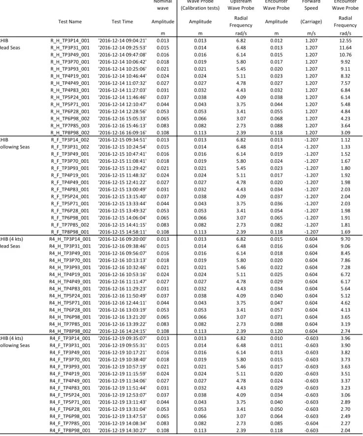
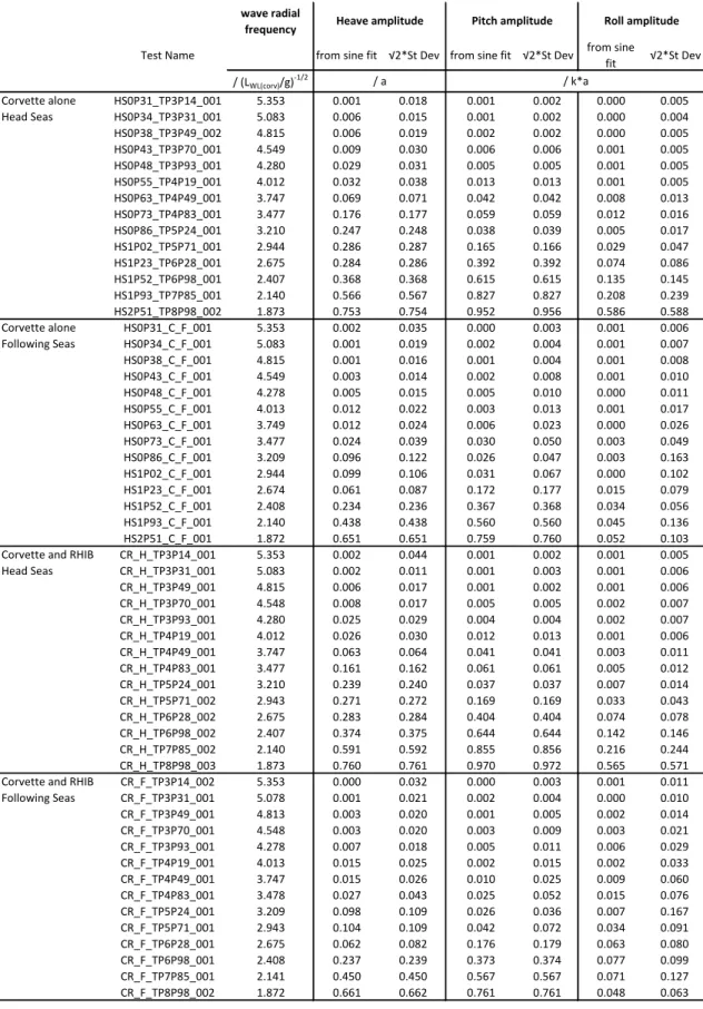
For consistency in comparing the different tests, the amplitude of the wave as measured during wave calibration was used to non-dimensionalize the motions, and not the

amplitude of the wave measured during each test. The nominal wave number was used to calculate wave slope. The measurements of encounter wave made during the tests were affected by the wave probe wire deflecting as the carriage moved, and by the presence of the model or by its wake in following seas. Test wave measurements are presented in Table 9 and Table 10.

Non-dimensional motion amplitudes (RAOs) were calculated using two different evaluations of motion amplitude:

• Motion amplitude derived from the standard deviation: √2 ∗ �� . This measure reflects the full magnitude of response, of any frequency.

• Amplitude of the sine function fitted to the motion. This isolates the motion response at the same frequency as the encountered wave.

(33)

Both are shown superposed on the RAO plots. Unfilled markers denote data calculated using the standard deviation.

Non-dimensional motion amplitudes of each vessel were plotted against the wave

circular frequency � non-dimensionalized by (�_��/�)−12, where �_�� is the waterline

length of the vessel. The frequency of the upstream wave probe was used. The relationship between non-dimensional circular encounter and wave frequencies is shown in Figure 18 for both the corvette and the RHIB. The plots also show the natural frequencies of the vessels.

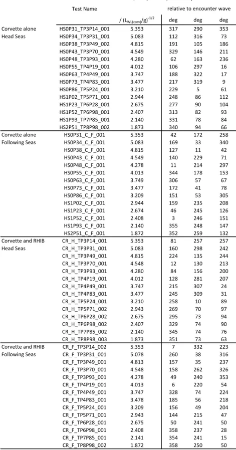
On plots showing the phase lag of the motions relative to the wave, unfilled markers denote test points for which the motion response was predominantly at frequencies other than the encounter wave frequency, and the phase measurement is not meaningful.

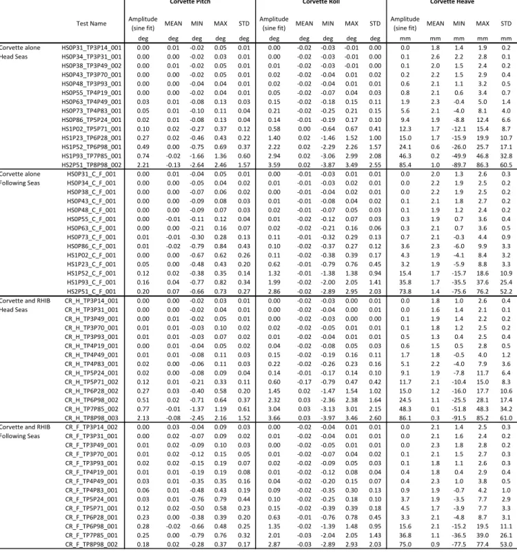
Figure 19 presents the heave, pitch and roll responses of the corvette at 8 knots in regular waves, in head seas and in following seas, alone and in the presence of the RHIB. Figure 20 shows the phase lags of the corvette motion responses relative to the wave. Non-dimensional radial frequencies up to 3.4 are usually needed for defining the RAO, and for the frequencies tested above this value, the motion responses of the corvette are small.

The non-zero roll motions of the corvette observed during the tests in head seas at the lowest tested frequencies are due to small physical asymmetries, along with the wave encounter frequency approaching the natural roll frequency of the corvette as seen in Figure 18.

As expected, the presence of the small RHIB alongside has a negligible effect on the motions of the larger vessel.

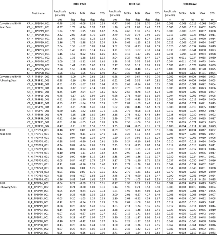
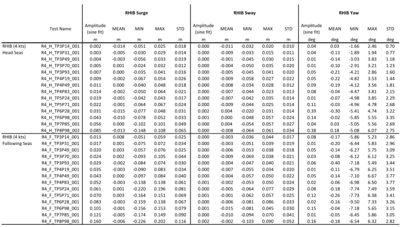
Figure 21 presents the heave, pitch and roll motions, and Figure 22 presents the surge, sway and yaw motions, of the RHIB at 8 knots in regular waves, in head seas and in following seas, both alone and alongside the corvette. The corvette has a strong

influence on all motions of the RHIB, except surge and sway in head seas. In some cases, the RHIB motions are attenuated by the presence of the corvette. This is the case for heave, pitch and surge motions in following seas. The roll and yaw responses are markedly increased by the proximity of the corvette, especially in head seas, as can be expected due to the wave generated by the corvette. In head seas, roll amplitude when the RHIB is alongside the corvette peaks at two frequencies: at non-dimensional radial frequency of 1.5, which corresponds to the natural roll frequency of the RHIB, and at a lower non-dimensional frequency of 0.8. The roll response of the RHIB alongside the corvette in head seas is strongly coupled with the RHIB yaw response. Figure 23 and Figure 24 show the phase lags of the RHIB motion responses relative to the wave.

(34)

The next set of figures examines the effect on the motions of the RHIB alone, of reducing forward speed from 8 knots to 4 knots. Figure 25 presents the amplitudes of heave, pitch and roll responses. Although its heading is parallel to the direction of the waves, the RHIB exhibits non-zero roll motions during the tests, due to unavoidable asymmetries, and to the free model not maintaining a perfect heading. Figure 26 shows the surge, sway and yaw amplitudes at either forward speed. The RHIB surge response in following seas is large at the normal operation speed of 8 knots but is significantly reduced at 4 knots. The surge gain parameters of the autopilot were kept identical for both speeds in following seas. Figure 27 and Figure 28 show the effect of forward speed on phase lag of the RHIB motion responses relative to the wave. For the RHIB alone, only phases for the motions in the longitudinal vertical plane are meaningful. Figure 29 shows the standard deviation of the RHIB driving parameters, in full scale units, as function of the wave frequency, for the RHIB alone at both speeds as well as alongside the corvette. The variations of steering angle amplitude are consistent with those observed for the yaw motion.

All results are also presented in tables. Tables from Table 11 to Table 15 show the measurements of motions for both vessels for each run, in model scale units, while Table 16 and Table 17 show the measurements of the RHIB driving parameters. Table 18 presents the non-dimensional motion amplitudes for the corvette, and Table 19 the phases of corvette motions relative to waves. Tables from Table 20 to Table 23 present the non-dimensional motion amplitudes for the RHIB, and Table 24 and Table 25 the phases of RHIB motions relative to waves.

8.2 Tests in irregular waves

Table 26 presents for each configuration tested the characteristics of the measured waves, both upstream and encounter, in full scale units, and compares them to the nominal and calibration values. These characteristics are results of zero-crossing

analysis, spectrum analysis, and statistics, on the merged time series for each condition. The required minimum of 100 wave encounters was met for every configuration and test condition.

Table 27 presents the characteristics of the response spectrum of the corvette

motions -notably significant height-, and statistical values of those motions, in full scale units, for each configuration tested. Significant heights of heave, pitch and roll are plotted in the two top plots of Figure 30. Consistently with the results of tests in regular waves, the corvette motions are not affected much by the presence of the RHIB

(35)

Table 28 shows the characteristics of the response spectrum of the RHIB

motions -notably significant height-, and statistical values of those motions, in full scale units, for each configuration tested. Significant heights of the RHIB motions are

presented plotted against forward speed in Figure 30. Roll and yaw are the motions most amplified by the presence of the corvette. Surge in following seas is reduced. These observations are consistent with the results of the tests in regular waves.

Finally, Table 29 shows the statistics of the RHIB shaft speed, steering angle and forward speed, in full scale units, for each configuration tested in irregular waves.

9 Conclusion

In conclusion, an extensive set of data was provided for validation of the numerical tool. The model tests quantified the motion responses for both vessels in the prescribed wave conditions, and quantified the effect of interaction. The motions most affected by the interaction were the roll and yaw motions of the RHIB.

10 Aknowledgements

The author would like to recognize the invaluable contribution that the numerous people in the project team made to the success of these model tests. The work of teams from the electronic and design and fabrication departments of NRC was instrumental for the success of the functional RHIB model, as was the work of the control specialists who developed the autopilot. The dedication of the tank technical personnel contributed greatly to the quality of the measurements.

11 References

1. “Construction of Models of Ships, Offshore Structures, and Propellers”, NRC OCRE Standard Test Method GM-1, V11, February 14, 2012.

2. “Environmental modeling – waves, Wind, Current”, NRC OCRE Standard Test Method GM-3, V6, March 2004.

3. “Seakeeping”, NRC OCRE Standard Test Method TM-5, V7, March 2012.

4. “Seakeeping Experiments”, ITTC – Recommended Procedures and Guidelines 7.5-02-07-02.1, 2014.

5. Mills, Jason. GDAC DAQ File Format Version 2, LM-2012-01, NRC-IOT, December 2011.

(36)

(37)

O CRE -TR -201 7 -0 08 6 D e fini tio n o f t he w a v e s Regular waves: wave steepness 1/ 50 circular

frequency ωfrequency f period T wave length λ wave height circular frequency ω

frequency f period T wave length λ wave height phase velocity group velocity wave number k λ /LWL λ /LWL

rad/s Hz sec m m rad/s Hz sec m m m/s m/s 1/m Corvette RHIB

0.7 1.429 8.98 125.7 2.51 2.39 0.380 2.633 10.814 0.216 4.107 2.063 0.581 1.79 15.12 0.8 1.250 7.85 96.3 1.93 2.73 0.434 2.304 8.285 0.166 3.596 1.799 0.758 1.37 11.59 0.9 1.111 6.98 76.1 1.52 3.07 0.488 2.048 6.546 0.131 3.197 1.598 0.960 1.08 9.16 1 1.000 6.28 61.6 1.23 3.41 0.543 1.843 5.301 0.106 2.877 1.438 1.185 0.88 7.41 1.1 0.909 5.71 50.9 1.02 3.75 0.597 1.675 4.379 0.088 2.614 1.307 1.435 0.73 6.12 1.2 0.833 5.24 42.8 0.86 4.09 0.651 1.536 3.682 0.074 2.397 1.199 1.706 0.61 5.15 1.3 0.769 4.83 36.5 0.73 4.43 0.705 1.418 3.138 0.063 2.213 1.107 2.002 0.52 4.39 1.4 0.714 4.49 31.4 0.63 4.77 0.760 1.316 2.703 0.054 2.054 1.027 2.325 0.45 3.78 1.5 0.667 4.19 27.4 0.55 5.11 0.814 1.229 2.358 0.047 1.918 0.959 2.665 0.39 3.30 1.6 0.625 3.93 24.1 0.48 5.46 0.868 1.152 2.071 0.041 1.798 0.899 3.033 0.34 2.90 1.7 0.588 3.70 21.3 0.43 5.80 0.922 1.084 1.834 0.037 1.692 0.846 3.426 0.30 2.57 1.8 0.556 3.49 19.0 0.38 6.14 0.977 1.024 1.637 0.033 1.598 0.799 3.839 0.27 2.29 1.9 0.526 3.31 17.1 0.34 6.48 1.031 0.970 1.469 0.029 1.514 0.757 4.279 0.24 2.05 2 0.500 3.14 15.4 0.31 6.82 1.085 0.921 1.324 0.026 1.438 0.719 4.746 0.22 1.85 Irregular sea-state: Bretschneider spectrum

Full Scale Model Scale

Hs 1.25 m Hs 0.1075 m

Tp 7.5 s Tp 2.200 s

Full Scale, deep water Model Scale, calculated for 7 m depth

(38)

Table 7 Autopilot gains

Test Name Surge Gain KDx Surge Gain Kix Surge Gain KPx Sway Gain Kiy Sway Gain Kpy

rpm*s/m rpm/m*s rpm/m °/m*s °/m CR_F_TP3P14_002 5 3 12 3 25 CR_F_TP3P31_001 5 3 12 3 25 CR_F_TP3P49_001 5 3 12 4 25 CR_F_TP3P70_001 5 3 12 4 25 CR_F_TP3P93_001 5 3 12 4 25 CR_F_TP4P19_001 5 3 12 4 25 CR_F_TP4P49_001 5 3 12 4 25 CR_F_TP4P83_001 5 3 12 4 25 CR_F_TP5P24_001 5 3 12 4 25 CR_F_TP5P71_001 5 3 12 4 25 CR_F_TP6P28_001 5 3 12 4 25 CR_F_TP6P98_001 5 3 12 4 25 CR_F_TP7P85_001 5 3 12 4 25 CR_F_TP8P98_002 5.697 0.0 9.398 4 25 R_F_TP3P14_002 5 3 12 4 25 R_F_TP3P31_002 5 3 12 4 25 R_F_TP3P49_001 5 3 12 4 25 R_F_TP3P70_001 5 3 12 4 25 R_F_TP3P93_001 5 3 12 4 25 R_F_TP4P19_001 5 3 12 4 25 R_F_TP4P49_001 5 3 12 4 25 R_F_TP4P83_001 5 3 12 4 25 R_F_TP5P24_001 5 3 12 4 25 R_F_TP5P71_001 5 3 12 4 25 R_F_TP6P28_001 5 3 12 4 25 R_F_TP6P98_001 5 3 12 4 25 R_F_TP7P85_002 5 3 12 4 25 R_F_TP8P98_001 5 3 12 4 25 R4_F_TP3P14_001 5 3 12 4 25 R4_F_TP3P31_001 5 3 12 4 25 R4_F_TP3P49_001 5 3 12 4 25 R4_F_TP3P70_001 5 3 12 4 25 R4_F_TP3P93_001 5 3 12 4 25 R4_F_TP4P19_001 5 3 12 4 25 R4_F_TP4P49_001 5 3 12 4 25 R4_F_TP4P83_001 5 3 12 4 25 R4_F_TP5P24_001 5 3 12 4 25 R4_F_TP5P71_001 5 3 12 4 25 R4_F_TP6P28_001 5 3 12 4 25 R4_F_TP6P98_001 5 3 12 4 25 R4_F_TP7P85_001 5 3 12 4 25 R4_F_TP8P98_001 5 3 12 4 25 CR_F_IRR_002 5 5 10 3 25 CR_F_IRR_003 5 5 10 3 25 CR_F_IRR_004 5 5 10 3 25 CR_F_IRR_006 5 5 10 3 25 CR_F_IRR_007 5 5 10 3 25 CR_F_IRR_008 5 5 10 3 25 CR_F_IRR_009 5 5 10 3 25 R_F_IRR_001 5 3 12 4 25 R_F_IRR_002 5 3 12 4 25 R_F_IRR_003 5 3 12 4 25 R_F_IRR_004 5 3 12 4 25 R_F_IRR_005 5 3 12 4 25 R_F_IRR_006 5 3 12 4 25 R_F_IRR_007 5 3 12 4 25 R4_F_IRR_001 5 3 12 4 25 R4_F_IRR_002 5 3 12 4 25 R4_F_IRR_003 5 3 12 4 25

* Gain values were being changed during test CR_F_TP8P98_002, but did not alter significantly the model tracking Sway gain D: 0 for all tests

H: head seas, F: following seas CR: corvette and RHIB R4: RHIB at 4 knots TP: wave period (full scale) IRR: irregular waves R: RHIB alone