Design and optimization of an MHD energy harvester for intelligent pipe systems

(1)

Design and Optimization of an MHD Energy

Harvester for Intelligent Pipe Systems

by

Xiaotong Zhang

Submitted to the Department of Mechanical Engineering

in partial fulfillment of the requirements for the degree of

Master of Science in Mechanical Engineering

at the

MASSACHUSETTS INSTITUTE OF TECHNOLOGY

June 2019

©

Massachusetts Institute of Technology 2019. All rights reserved.

Signature redacted

A uthor ... ...

(I I

Department of Mechanical Engineering

May 17, 2019

CSignature

redacted

C ertified by .... ...

Kamal Youcef-Toumi

Professor

Thesis Supervisor

Signature redacted

...

.

. . . ....

.

Nicolas Hadjiconstantinou

Chairman, Committee on Graduate Students

Accepted by ...

MA I UTE

JUN 13 2019

(2)

(3)

Design and Optimization of an MHD Energy Harvester for

Intelligent Pipe Systems

by

Xiaotong Zhang

Submitted to the Department of Mechanical Engineering on May 17, 2019, in partial fulfillment of the

requirements for the degree of

Master of Science in Mechanical Engineering

Abstract

In this thesis, an innovative Magnetohydrodynamic (MHD) energy harvester with the use of the magnetic concentrator is designed and optimized. A theoretical model relating the conductivity of water, magnetic flux density B, flow velocity u and the channel volume to the power output is first established. This leads to the decoupled analysis and simulations of magnetic field and flow field. The prototyped energy harvester without the concentrator achieves a power output of 442 nW, while the power output of the final design with the concentrator is expected to be 718.5 nW. The concept of another MHD energy harvester with a spiral flow diverter is also established with hollow space in the middle of the energy harvester for flow and robots to pass through. It is validated by CFD simulations that the flow velocity in the channel surrounding the hollow area is greatly amplified with the spiral flow diverter. The MHD energy harvester with the concentrators and spiral flow divereter is expected to produce power output of 238.3 nW.

Thesis Supervisor: Kamal Youcef-Toumi Title: Professor

(4)

(5)

Acknowledgments

First of all, I would like to thank my advisor Prof. Kamal Youcef-Toumi for his guidance and support through my two-year study at MIT. Without his help and guidance, my successful transition from my undergraduate focus Computational Fluid Dynamics to mechatronics and robotics would not have been possible. The spirits of persistence and seeking the truth he conveyed are also great treasures for my career and professional development.

I also would like to thank Dr. You Wu, Steven Yip Fun Yeung, Tyler Takeo Okamoto, and Elizabeth R Mittmann, who work together with me in the same project and offer me valuable advice and assistance. I am also thankful to the other mem-bers of the MIT Mechatronics Research Laboratory. They are great engineers and researchers. I learned a lot of knowledge and obtained some fabulous inspiration from discussions with them.

I am also thankful to MathEarth Inc., who sponsors the project kindly. The staffs

there, including Dr. Haoping Yang and Mr. Honghai Bi, provide deep industrial insights and experiment supports, which are significant for the results in this thesis and are also gratefully appreciated.

Last but not least, I must sincerely and especially thank my parents, Mr. Hongda Zhang and Ms. Fenghua Zhu, for their constant encouragement and support from China. And I am also thankful to all my friends, who accompany me and make my life fun every day.

(6)

(7)

B .7 Sum m ary . . . . 93 . . . . 93 . . . . 94 . . . . 95 . . . . 95 . . . . 96 . . . . 97 . . . . 98 . . . . 99 . . . . 100 . . . . 101 . . . . 101 . . . . 104 . . . . 104 . . . . 107 . . . . 109 . . . . 109 C Materials and Components

C.1 Conductive Coating . . . . C.2 Smooth-on XTC-3D Coating . . . . 79 79 80 81 . . . . 8 1 . . . . 8 2 . . . . 8 4 . . . . 9 0 111 111 113 Detector

(10)

(11)

List of Figures

2-1 Schematic of a simplified MHD energy harvester. . . . . 25 3-1 The relationship between the averaged B within the channel and the

distance between two magnets with d = 0.002m, and unit m = 1A -m2 3 5

3-2 Magnetic flux induced by two strong Neodymium magnets. . . . . 37

3-3 Magnetic flux with an additional three-layer magnet structure. . . . . 38

3-4 Front view of the concentrator design . . . . 40

3-5 Demagnetization curve for N42 grade Neodymium magnets. . . . . . 41

3-6 Magnetic flux vector plot. (a) only magnets; (b) magnets and inner

concentrator; (c) magnets, inner concentrator, and loop with width w = 0.005 m . . . . 41

3-7 Contour of magnetic flux density in y-direction. (a) only magnets; (b) magnets and inner concentrator; (c) magnets, inner concentrator, and loop with width w=0.005 m. . . . . 42

3-8 B-H curve of mu-metal and Metglas. (a) overview; (b) detailed view. 43

3-9 Contour of magnetic flux density in y-direction. (a) metglas; (b)

mu-m etal. . . . . 44

3-10 Magnetic flux vector plot. (a) metglas; (b) mu-metal . . . . . 44

3-11 Contour of magnetic flux density magnitude. (a) metglas; (b) mu-metal. 45

3-12 Average By in the channel with various loop widths. . . . . 46

3-13 Magnetic flux density contour for the cases with loop size of (a) 0.002

m ; (b) 0.015 m . . . . 46

(12)

3-15 Magnetic flux vector with and without two big magnets outside. . . .

4-1 Working curve of a typical centrifugal pump. . . . . 52

4-2 Computational region schematic and mesh. . . . . 54

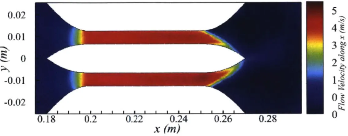
4-3 The contour of u_- in the case with 7 mm channel and 10,000 pa inlet pressure on the slice z=0. . . . . 55

4-4 Static pressure contour in the case with 7 mm channel and 10,000 pa inlet pressure on the slice z=0. . . . . 56

4-5 Force acting on the energy harvester in the x-direction. . . . . 56

4-6 Averaged u, within the channel. . . . . 57

4-7 Contour of u, with fixed h=7 mm and 20,000 Pa inlet pressur inlet. (a) b=30 mm, (b) b=25 mm, (c) b=20 mm, (d) b=15 mm, (e) b= 10

m m , (f) b=5 m m . . . . . 59

4-8 Averaged u, within the channel with various channel width b. ... 60

4-9 Moody chart for pipes covered with sands. . . . . 61

5-1 Final design. (a) overall view; (b) side view; (c) front view; (d) magnets

and concentrators . . ... . .... .. . . 64

5-2 Material test of the conductive coating. . . . . 65

5-3 Fabrication of components and assembled prototype. . . . . 67

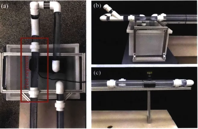
5-4 Experimental setup. (a) top view of the tank, pump and test segment;

(b) front view of the tank, pump and test segment; (c) flow meter 2 m

after the pipe elbow . . . . 68

5-5 Experimental and theoretical power output with various load resistance. 70 5-6 Preliminary design of the energy harvester with a hollow area in the

cen ter. . . . . 73

5-7 Design of the spiral flow diverter and cross section of the turbulence

inducer. ... .... .74

5-8 Mesh for spiral flow diverter case. (a) overview; (b) zoom-in view on

slice of y=0 m (middle plane). . . . . 75

(13)

5-9 Pressure contour at x=0.39 m from the energy harvester inlet for the

case (a) with spiral flow diverter; (b) without spiral flow diverter. . . 75

5-10 Streamline for the case (a) without spiral flow diverter; (b) with spiral flow diverter. . . . . 76

5-11 Velocity contour at the slice xz=0.39 m from the energy harvester inlet for the case (a) with spiral flow diverter; (b) without spiral flow diverter. 76 5-12 Velocity contour at the slice y=0 m (middle plane) for the case (a) with spiral flow diverter; (b) without spiral flow diverter. . . . . 77

A-I Concentrator geometry and parameters. . . . . 82

A-2 B-H curve of the metarials . . . . 83

A-3 Demagnetization curve for N42 grade Neodymium magnets. . . . . . 83

A-4 Contour of B magnitude. (a) mu-metal concentrator; (b) without con-centrator (material in the trapezoidal concon-centrator region assigned as a ir). . . . . 8 4 A-5 Contour of directional B. (a) mu-metal concentrator; (b) without con-centrator (material in the trapezoidal concon-centrator region assigned as a ir). . . . . 8 5 A-6 Averaged By in the channel with the concentrator of (a) mu-metal with 2 mm height; (b) mu-metal with 8.5 mm height; (c) permalloy with 2 mm height; (d) permalloy with 8.5 mm height; (e) annealed pure iron with 2 mm height; (f) annealed pure iron with 8.5 mm height. .... 86

A-7 Difference of averaged By between mu-metal and (a) permalloy with 2 mm height; (b) annealed pure iron with 2 mm height; (c) permalloy with 8.5 mm height; (d) annealed pure iron with 8.5 mm height. . . . 88

A-8 Max averaged By for concentrators with height of (a) 2 mm; (b) 8.5 mm. 89 A-9 Difference of averaged By between 2 mm and 8.5 mm height concen-trators. . . . . 89

A-10 Averaged By for 2 mm height concentrator with mu-metal. . . . . 90

(14)

B-i Working principle and prototype of previously designed leak detection

rob ot. . . . . 96

B-2 Simulation setup. (a) geometry setup. (b) mesh setup and refinement. (c) geometry zoom-in at the leak and the channel. . . . . 98

B-3 Simulation result for validation. (a) streamline without channel. (b) streamline with channel. (c) pressure contour without channel. (d) pressure contour with channel. (e) pressure distribution along the cen-ter line of the channel. (f) velocity distribution along the cencen-ter line of the channel . . . . 99

B-4 4 mm channel simulation result with various gaps. (a) no gap. (b) 1 mm gap. (c) 2 mm gap. (d) pressure distribution on the center lines of the channels. . . . . 100

B-5 2 mm and 8 mm channel simulation result with various gaps. (a) 2 mm channel no gap . (b) 2 mm channel with 1 mm gap. (c) 2 mm channel

with 2 mm gap. (d)8 mm channel with no gap. (e) 8 mm channel with 1 mm gap. (f) 8 mm channel with 2 mm gap. . . . . 102 B-6 1 mm gap simulation result with various channel sizes of (a) 2 mm

channel; (b) 4 mm channel; (c) 8 mm channel size; (d) 16 mm channel size. (e)plot of the pressure on center line. . . . . 103 B-7 Simulation results of cases with a 8 mm leak and 2 mm channel at

different position of (a) 1/4 of the leak; (b) 2/4 of the leak; (c) 3/4 of the leak; (d) 4/4 of the leak. . . . . 104 B-8 Simulation results of cases with a 8 mm leak and 2 mm channel skewing

450 to the right at different position of (a) 1/4 of the leak; (b) 2/4 of the leak; (c) 3/4 of the leak; (d) 4/4 of the leak. . . . 105 B-9 Working Principle of the Overset Mesh Method. . . . . 106

B-10 Simulation results of moving channels using Overset Mesh Method. 106

B-11 Proposed conceptual design. . . . . 107

(15)

List of Tables

3.1 Permeability of typical materials. . . . . 39

3.2 Simulation results for effect validation. . . . . 42

C.1 Properties of the silver conductive coating material. . . . . 111

C.2 Properties of the nickel conductive coating material. . . . . 112

C.3 Properties of the carbon conductive coating material. . . . . 112

(16)

(17)

Chapter 1 Introduction

Sufficient and sanitary water supply is crucial for life, industrial production and eco-nomic development. But a huge amount of water is wasted due to leak every day around the world. Although some technologies have been developed to alleviate this problem, there's still a long way to achieve a much more sustainable, environmentally friendly, and resource conservative water distribution system. And this system can be a significant part or a good start point of a smart city, monitoring the working condition of assets with IoT (Internet of Things) sensors and data transmission.

1.1 Background and Motivations

20% of water in the distributing pipe system is wasted every day around the world due to underground leaks, which are even hard to find [1]. The problem in developing countries are even worse. In 2016, it was reported by the World Bank that about 45 million cubic meters of water are lost daily in developing countries, which is worth an economic value of over 3 billion USD per year [2]. On the other hand, those coun-tries need to face tremendous water demand brought by the large-scale population and widespread heavy industry. Besides water resource loss, the pipe leaks might also cause severe damage to private properties and public infrastructures, which is estimated to cost billions of dollars within the US [3].

(18)

possible solutions to settle the problems by realizing real-time monitoring or even prognostics of the pipe working condition. And the water quality can even be mon-itored. The smart pipe systems not only can conserve water resource for the earth, but also means dramatically reduced economic loss and more profit for the water authorities. Thus great interest in this area has been aroused in the past few years.

Such a system can be composed by several components, including sensors, data transmission, working condition recognition, system failure alarm, and energy har-vesting. And the energy harvesting component can be the bottleneck for most of such systems since it is sophisticated to supply power for the sensors widely spread every-where under the ground around the cities with conventional methods, like batteries or wires. And those methods also demand a lot of manpower to maintain. Thus a de-vice to harvest energy from environment continuously for a long time, and providing power for the sensor, is desired. And it attracts more and more focus and attention from both academia and industry.

Thus, in this thesis, we will focus on the design and performance optimization of an energy harvester extracting power from the water flow and providing power for leak detection sensors along the instrumented pipes.

1.2 Previous Studies on Smart Pipe Systems

The working principles and characteristics of sensors detecting leaks based on acous-tics, pressure gradient, Ground Penetrating Radar, fiber optic sensing, and force sensitive resistors are discussed in Section B.1. The development of these sensors and the algorithm to process their data makes it feasible to realize real-time monitoring in practice.

And then, a bigger goal is raised for such systems to achieve monitoring with ultra-low power consumption. It is found that most asset failure takes days, weeks, or even months to happen. Thus it is useless to monitor and run all the functions continuously all the time

[4].

It is calculated that a continuous monitoring system (including ZigBee communication, sensors, and local microprocessors) can consume

(19)

power as low as 20 mW for one node, and if the system only works 100 ms per day, it will give a power requirement of only 20 nW

[5].

In 2014, based on this idea, a novel sensor using force sensitive resistors is developed by Ali M. Sadeghioon, Nicole Metje, David N. Chapman and Carl J. Anthony from University of Birmingham. After converting the flow pressure into strain of the pipe, the sensor measures the flow pressure fluctuation every 6 hours with a minimal 2.2 puW power consumption. And the pressure information can also be used to locate the leaks

[6].

This work validated the feasibility to monitor the pipe working condition with a low-frequency sampling. And it also promises the practical use of the energy harvester developed in this thesis in real scenario. With the advancement of MEMs and researches on the ultra-low power consumption sensors, this power requirement can be even lower in the future and the sacrifice on the sample rate can be eliminated.

The existence of these sensors provides a lot of space for novel energy harvester design that may be trivial in the past.

1.3 Previous Studies on Energy Harvesting

The energy source of the sensors used are batteries. But the cost to replace the underground batteries at a regular schedule is unaffordable for most water companies, which forces the research related to energy harvesters converting the flow kinetic energy to electrical energy. These previous researches can be sorted out into four categories based on the working principles.

1.3.1 Turbine

The first kind of energy harvesters implements conventional water turbines or impeller wheels. The turbines can convert the directional velocity of the flow to rotational mo-tion of the turbine. And this rotamo-tional momo-tion will result in the relative momo-tion be-tween the magnets and coils, which can be seen as the prerequisite of electromagnetic induction.

(20)

require-ment of a sensor node. But this methods can also face some disadvantages. Firstly, the turbines rotate all the times, which means regular maintenance is inevitable. This may not be a problem for wind turbine or dam turbine which works above ground, but is extremely difficult for underground pipe systems. Secondly, the turbine blades can be damaged by the sudden pressure fluctuation within the pipeline or foreign objects moving together with flow. Thirdly, it can also bring in vibrations, causing rapid fatigue on pipe structure or unacceptable noise to the sensing data [7, 8].

1.3.2 Direct electromagnetic induction

The second category of energy harvesters for wireless sensor networks adopts direct electromagnetic induction principle by driving permanent magnets or coils to vibrate among or next to coils or permanent magnets. The vibrations can come from the locomotion of vehicles or humans, or the pressure ripple within pipe flow. The power output is usually optimized by tuning spring constant and mass to harmonic [9, 10,

11]. A good design can usually achieve tens or hundreds of microwatts only on one

PCB board.

But these methods also introduce extra vibrations into the system. And the device after deployment only corresponds to one optimal vibrational frequency, which greatly limits the range of flow velocity and pressure within the pipeline.

1.3.3 Piezoelectric effect

Piezoelectric effect is the phenomenon and ability of some materials that electric charges can be generated on the material surface in response to mechanical stress. To extract the charges continuously, vibrational motion is usually loaded on the material. And then positive and negative charges are generated on the surface alternately, which can produce alternating current out from the materials.

The vibration can come from a wide source, including human stepping on shoes or vehicle locomotion. When used in pipe systems, it can also come from the dynamic pressure ripple or the artificial vibration induced by specially designed fluid-structure

(21)

interaction and asymmetrical vortex shedding. Using the pressure ripples, a piezo-electric material stack together with its housing, which can be mounted on the pipe, is already designed and prototyped. And this prototype finally achieves a 1.2 mW max power output [121. As for the source of the induced vibration, an energy harvesting eel, composed of flexible piezoelectric membrane PVDF and a bluff body acting as the excitation of the Karman vortex street, is proposed in 2001 [13, 141. But the eel has not been prototyped, and thus there's no experimental demonstration of the concept.

This method can also introduce vibrations to the structure and noise to the data recorded by sensors. Moreover, since the vibrational frequency of the wake behind the bluff body is regulated by Strouhal number and flow velocity, the tuning of design parameters also highly depends on the flow velocity, which means one device can only work best for one specific velocity and the power output may be trivial under other velocities. However, it is hard to set the flow velocity fixed as most water distribution systems have peak and valley time. Also, design with piezoelectric material also needs to deal with off-resonance, as the pressure fluctuation frequency is usually much smaller than the fundamental resonance of the piezoelectric material.

1.3.4 Magnetohydrodynamics

No matter which concept is adopted to harvest energy, the basic principle is that moving charged particles, in the presence of magnetic field, experience a force in the direction perpendicular to both magnetic flux density B and the charge velocity u. One way that is more direct to produce electricity than the above three methods is to induce electric field by the fact that positive and negative charges tend to move in opposite directions in the influence of B field, which is referred to as MHD (Magneto hydro dynamics) effect.

This phenomenon is first observed by Faraday in 1831, when he placed two large electrodes in the Thames river and connected them to a galvanometer. The conduct-ing water flowed between electrodes and through earth's magnetic field. An irregular and small signal is observed [151. Years later, the same principle started to be used in

(22)

large power plants, but with stronger magnetic field and highly conductive conduc-tors. In 1961, a liquid fossil fuel "seed" with a potassium compound was utilized and the equipment successfully achieved power levels more than 10 kW [161. After that, MHD power generators have been widely studied, and the MHD/Steam binary cycle power plant can even reach an efficiency of 60%

[17].

Conversely, MHD principle can also be used for ship propulsion in seawater with high conductivity and salinity [18]. In 2000, a one-ton ship model in China is propelled

by MHD propulsion to a speed of 0.61-0.68 m/s [19].

However, large power output or propulsion force usually requires superconducting coils to provide stronger B and conductors with high conductivity, such as plasma or sea water. These two factors both limit the use of MHD. However, with the ad-vancement of electronic engineering and leak detection algorithm, the power demand for each sensor node on smart pipes can achieve as low as 2.2 pW

[6],

which makes MHD power generation for wireless sensor networks feasible after careful design and optimization.

There are no moving parts in a working MHD energy harvester except for the conductors, and the power output does not depend on the flow condition in frequency domain. These two characteristics overcome the shortcomings of the above three methods of frequent maintenance, additional vibrations, off-resonance of piezoelectric material, and high dependence on the vibrational frequency. Thus MHD shows a great potential in energy harvesting than other methods in the applications where high reliability and automatic adaptation to different flow conditions are desired.

1.4 Contribution and Thesis Outline

In this thesis, a novel MHD energy harvester working with tape water and permanent magnets in room temperature is proposed, prototyped, and tested. And this is the first ever prototyped and tested MHD energy harvester for smart sensor networks, to the best of our knowledge.

(23)

struc-ture and magnetic concentrators with high permeability are added in the design. A methodology to optimize the overall performance of such an energy harvester under different pipe sizes and flow condition is also proposed and validated.

Moreover, a new concept design is also proposed. In this design, the energy harvester has a hollow area at its center to allow the flow and robots to go through without any interruption. And the flow diverter used in this concept design can also be used in other applications, where flow needs to be diverted from its original flow pattern.

The thesis starts from the theoretical model governing the MHD phenomenon in Chapter 2. And it is found that the power output is proportional to the square of both the magnetic flux density and the flow velocity. Based on this, magnetic field and flow field are optimized in Chapter 3 and 4 using theoretical analysis and numerical simulations. In Chapter 5, an MHD energy harvester with the novel design after optimization is proposed. And its simplified version is prototyped, and tested in the experimental setup built at MRL. Methods to further improve the results from the prototype in practical use are analyzed and suggested using the model established in Chapter 2. The new flow diverter and the energy harvester with hollow center are also described and analyzed in Chapter 5.

(24)

(25)

Chapter 2 MHD Energy Harvester Modelling

MHD is the macroscopic behavior of Lorentz force acting on charged particles. Even in ultrapure water, the existence of the self-ionization balance reducing water molecules into hydroxide ions and hydrogen ions results in a conductivity about 0.055 pS/cm.

Daily tap water can even reach a conductivity of 50-800 pS/cm due to impurities.

A simplified Faraday energy harvester is shown in Figure 2-1, with two

elec-trodes perpendicular to the z-axis, conductor flowing in the x-direction, and B in -y-direction. The geometric parameters illustrated in the figure are also used in the following system modelling and analysis.

Electrode

current (z)

magnetic flux (-y)

(26)

2.1 Generalized Ohm's Law

Under the assumption that Hall effect of the induced current is neglected, the in-duced current density vector can be described using the generalized Ohm's law as in Equation (2.1), that

J = a(E+ u x B) (2.1)

where a (S/m) is the conductivity, J (A/m2) is the current density vector, E (V/m) is the electric field intensity, u (m/s) is the velocity of the conductor, and B (Wb/m2₎

is the magnetic flux density vector. The term u x B represents the additional Lorentz force in the direction perpendicular to both u and B, or the additional induced electric field in the fixed coordinate system after coordinate transformation from the moving coordinate system. And the term E comes from the potential difference between the two electrodes. In our following discussion, we will assume that all the parameters are uniform and their values are averaged among the region.

In this particular problem, the current density in the z-direction, which can be collected by electrodes, can be deduced to a scalar expression in Equation (2.2).

Jz = a(Ez - uB) (2.2)

where subscript z represents the component in the z-direction of a vector. Thus the open circuit electric field should be uB for open circuit, where Jz = 0. While

for the short circuit circumstance Ez = 0, the short circuit current density should be -uuB.

2.2 Power Extracted

The geometric parameters of a conductor channel are shown in Figure 2-1. h and b represents the height and width of the channel respectively, and L is the length of electrodes in the direction of flow.

(27)

re-sistor Rload _{is installed in the circuit to extract power out of the generator. With}

simple manipulation, the total power output can be deduced by using I = J2 - h - L (conservation of charge), and V = E2 b = I(Road

+

Rj) (definition of electric field

and Ohm's law for external circuit), where Ri is the internal resistance, and I and V,2 are the current and voltage output from the generator. Then the current output and power extracted by the load resistor can be derived in Equation (2.3) and Equation

(2.4).

uhLbuB

2b + -hLRoad

chLbuB -12

Pout = b hLRuo Rhoad (2.4)

.2b + ah LRioad -with a maximized power output expressed by (2.5)

Pmax = bhL U2B2 (2.5) 8 when 2b Road = b (2.6) orhL

And it also should be noticed that the power extracted is proportional to the channel volume. This allows the power output to be magnified in real scenario where the sizes of pipes and harvesters are way bigger than the ones in the lab. But this also increases the difficulty to balance all the parameters, since large volume may result

in a smaller B.

2.3 Power Generated

The power extracted is different from the power that is generated in the whole system. Due to the existence of the internal resistance, there must be parts of the power dissipated. And in this case, the current and the power generated can be deduced as

(28)

in the Equation (2.7) an Equation (2.8)

I = hLbB (2.7)

2b + ohLRoad

Pgen = [ b (Road + Rj) (2.8)

2b + ohL Road

where Ri is the internal resistance, which can be written as

1lb

Ri -- b(2.9)

a hL

And then the maximized power generated can be derived and expressed by Equa-tion (2.10)

Pmaxgen = C Us B 2 (2.10)

4

when

Road = 0 (2.11)

The max power generated by the harvester is double of the max power extracted

by the load resistors. But the problem to use power generated as the result parameter

is that this parameter is hard to be measured and thus compared with the theoretical model. And the power consumed by the internal resistance is useless for practical use. Thus the power extracted in Section 2.2 will be the parameter we focus on and optimized in the following chapters.

2.4 Hall Effect

Another factor which may influence the result is the hall effect caused by the induced current in the direction of z-axis. This hall effect can cause another induced current in the direction of x-axis, which can reduce the flow velocity. After considering this effect, the current density in z-direction can be deduced to be

(29)

Jz ₁₊₀₂o 2 (Ez -uB + Ex) (2.12)

Jx 1 2(Ex -/3(Ez - uB)) (2.13)

And then the max power output can be calculated as

uobhLu2B2 _(2.14)

Pmaxout 8 + 4#3

where

3

is the hall parameter of the conductor flow defined as

#

= eB (2.15)

mev

where e is the atomic unit of charge; me is the electron mass; v is the collision frequency within the conductor.

The existence of the hall effect makes a change in the expression of the current and the power output. And it has to be considered in conventional MHD power generator working with "seeded" plasma, as the hall parameter in plasma can easily reach to 6 or 7.

However, in our design and optimization analysis with the conductor of water, this effect is neglected, and Equation (2.5) and (2.6) are adopted according to the following two reasons:

1) The hall effect for water is not so observable. In other words, the hall parameter

for water is very low.

2) Hall effect can be eliminated if the electrodes are segmented into pieces. In this case, the electrodes in x-direction are taken as open, and thus Jx = 0. And then it is derived that

Ex= g(E2 - uB) (2.16)

If the Equation (2.16) is substituted into Equation (2.12), the current density in

(30)

proved that the utilization of segmented electrodes will greatly eliminate this effect, although this kind of electrodes is not prototyped in this thesis due to fabrication limitation.

2.5 Discussion

Equation (2.5) shows that the result can be decoupled into velocity field u and mag-netic flux density field B, which both have a quadratic contribution on the power output. Thus, the power output can be dramatically magnified if B and u are opti-mized. And the optimal load resistor can be determined with Equation (2.6). How-ever, since the smart pipe system will deliver water for drinking and other daily use, it is very difficult to add seeds to increase water conductivity, like what other MHD power generators do. Thus, only u, B, and the channel geometry can be played with and optimized.

We can further represent u in the channel in Equation (2.5) with far-field velocity no and far-field cross-sectional area AO, using mass conservation AouO = ubh, and get

Equation (2.17)

o-A 2U2 L 2

Pmax 8 bB2 (2.17)

8 bh

which means that smaller b, smaller h, and longer L will maximize the power output under the assumption that the flow is incompressible and the geometry doesn't influence far-field flow velocity. However, the second assumption is not always true as most pumps provide pressure, and the same far-field velocity uo is hard to maintain

with high block aspect ratio and smaller size channel according to Poiseuille's law. In this case, theoretical analysis and CFD (Computational Fluid Dynamics) simulation with the controlled same inlet pressure is performed and discussed in the following chapter.

(31)

2.6 Summary

In this chapter, generalized Ohm's law is adopted first to describe the macroscopic behavior of the charged particles within water and the phenomenon of MHD. Based on that, the power that can be extracted by external resistors are deduced and it is found that B and u are two decoupled fields which both have a second order contribution on the power. Thus B and u are two fields to be specially analyzed and optimized in the following chapters. And it is also noticed that the power generated is proportional to the channel volume, which can't be ignored.

Hall effect of the induced current is also discussed. But this effect is not necessary to be taken into consideration at this stage since the hall effect of water is not very observable and it can be eliminated by segmented electrodes in the future.

(32)

(33)

Chapter 3 Magnetic Field Analysis and

Optimization

Based on the analysis in the above chapter, magnetic field B must be carefully dis-cussed and analyzed, since it can cause a significant difference in the power output.

3.1 Problem Description

To get the optimal B, key factors influencing B should be analyzed with both theoreti-cal and simulational methods. And some special designs, like magnetic concentrators, can also be assembled in the design to achieve an overall best optimization.

The magnetic field B is first built by two N52 degree Neodymium magnets with the size of 0.0762 m x 0.0762 m x 0.0127 m (3 inches x 3 inches x 0.5 inches), placing out of the pipe, which is the simplest magnet layout. Both magnets are very strong with a residual induction of 14,800 Gauss and a max surface induction of 2,125 Gauss when measured with a Gauss meter. The problem is that although the magnets are strong enough, the magnetic induction within the pipe is still measured to be small. The reason and solution to this problem should be discussed and proposed.

Moreover, a magnetic concentrator made of some materials with high magnetic permeability is commonly used in the design of transformers or sensors to concentrate or guide the magnetic flux, and thus to achieve a lower power dissipation or noise

(34)

level. But several factors, including the shape and the material of the concentrator, and the size of the flow channel, can all influence the effect. Thus a careful and systematical analysis of these parameters should be carried out.

3.2 Magnet Layout Design

In this section, a better design of magnet layout is proposed and validated after theoretical analysis and simulations.

3.2.1 Theoretical modeling

The theoretical modeling part is to model the magnetic field distribution amongst the channel and the whole space. Since the relative permeability of air, water, and PVC is very close to 1, all the materials, except for the magnets, are treated as vacuum with a relative permeability of 1.

According to the Gilbert model, a magnet can be modeled by a magnetic dipole, whose two poles are the magnetic sources with the same magnitude, but opposite signs. The magnetic vector potential in vacuum and the induced magnetic induction can be expressed by Equation (3.1) and (3.2) in polar coordinates.

A (r)- o m x r po m x r (3.1)

27rr2 r 47 r3

B(r) = x A = o(3r(mr) m) (3.2)

47 r5 r3

where A is the magnetic vector potential, B is the magnetic flux density, m is the magnetic moment, r is the displacement vector of a point in the space relative to the dipole, and

so

is the vacuum permeability constant. To further simplify the model for our analysis, we assume that the size of the magnets is much larger than the flow channel. The B at the same height is represented by the value of B on the center line connecting two magnets, which is shown in Equation (3.3):

(35)

po m po m

B(y) = _27r (+ ) (3.3)

y3 27r (R - y)3

where R is the distance between two dipoles, and y is the relative height of the point we concern from the lower magnet.

And then the averaged B in the vertical direction along the center line can be cal-culated, which is the parameter directly related to the power output. Since Equation

(3.3) shows two singularity point at y = 0 and y = R, we have to avoid

calcula-tion on these two points. Thus, B is integrated and averaged from y = 0.002m to

y = R - _{0.002m, where the distance 0.002 m can be considered as the wall thickness.} The relationship between the averaged B within the channel and the distance between two dipoles R is then obtained and shown in Figure 3-1.

30 R-d IF- 25 Bavg

= RB(y)dy

20 15--oR 10 0 0 0.02 0.04 0.06 0.08 0.1

R distance between magnets (m)

Figure 3-1: The relationship between the averaged B within the channel and the distance between two magnets with d = 0.002m, and unit m = 1A m2_.

In the figure, it is clearly shown that the theoretical averaged B decays dramati-cally with distance R.

(36)

3.2.2 Three-layer magnet layout design

Since the distance between the two magnets has a significant effect on B, two magnets should be kept as close as possible. However, such two big magnets are very difficult or impossible to be placed in a 2-inch pipe.

To achieve such a close distance and the thereby higher B field, a novel design is proposed that three layers of thin magnet plates are placed within the channel. And the three layers of magnets will form two separate water channels for the flow to run through. To make the design feasible for prototyping, every thin magnet plate is replaced by two thin magnet bars, which can be purchased easily online. Limited

by the round shape of the pipe, the bottom and top magnet plates are smaller than

the middle one. Thus the two kinds of magnet bars are with the size of 0.0508 m x

0.0127 m x 0.0032 m (2 inch x 0.5 inch x 0.125 inch), and 0.0508 m x 0.0095 m

x 0.0032 m (2 inch x 0.375 inch x 0.125 inch), respectively. The material of all the magnets is Neodymium.

As the geometry of such a layout is too complicated for the theoretical calculation, the effect of such a design will be verified by magnetostatic simulation.

3.2.3 Simulation setup

The simulations in this part are performed on ANSYS AIM R19.2, with a built-in permanent magnet simulation module.

Since the simulations here are only to verify the design, only two 3D cases are carried out. The first case contains only two big magnets outsides the pipe, while the second case also includes the three-layer magnet within the pipe. The sizes of all the magnets in the simulation are the same as the real magnets. And the distance between two adjacent magnet layers is set to be 11 mm, which is composed by one

7 mm water channel and two 2 mm wall thicknesses. Although the B field can be

further improved without the wall between the magnets and the water channel, a gap between them is still retained to avoid the damage to the magnets, and maintain the magnetic field in a long time.

(37)

Since the electromagnetic permeability of air, water, PVC, and ABS is very close, only the physical model of the magnets is established in the simulation. And all the other parts are set to be filled with air.

3.2.4 Simulation results

The magnetic flux density distribution in the space is simulated. After the simula-tions, B field and magnetic flux between the two strong magnets are shown in Figure

3-2. In the figure, it is observed that almost all the magnetic flux surrounds the

mag-nets, and B between two magnets are relatively small. B at the center point (shown as the red dot in Figure 3-2) of this case is calculated to be 0.115 T.

0.3

0.2 z

0.1

Figure 3-2: Magnetic flux induced by two strong Neodymium magnets.

The result of the second design with small magnets are shown in Figure 3-3. It is clearly shown that B in the region not close to the small magnets, is very similar to that in the first case. But B between the small magnets is dramatically amplified, indicated by both the more intensive flux and the red color. From the vector plot, it is also verified that the B field is very sensitive to the distance. And the changes far away from the magnets is difficult to function.

(38)

~Ow /*1,

<"S

~ U,~.; k

\

\\

L\:

t/ Jffl/

'

Figure 3-3: Magnetic flux with an additional three-layer magnet structure.

as the black dot in Figure 3-3) is calculated to be 0.27 T, which is increased by 2.45 times, resulting in a magnification of 6.00 times on the power output.

Thus the magnification effect of such a design on the B field is validated and this magnet layout will be used in the following discussion and the final design. Although only two cases are simulated here, the results and the conclusions should be generic for the cases with a reasonable variation of the parameters in the cases.

3.3 Magnetic Concentrator

The B field can be further optimized by a magnetic concentrator with the shape of trapezoid, which can concentrate the flux by adopting a gradually shrinking profile and material with high magnetic permeability. Material, such as Metglas, can achieve a relative permeability up to 1,000,000 at 0.5 T magnetic field. And the permeability of some typical materials are listed in Table 3-1.

With material like this, the magnetic flux can be guided and thus its density dis-tribution within the space can be controlled. In this section, a magnetic concentrator to enlarge the average magnetic flux density B in the channel is proposed and several parameters are analyzed for a better performance.

4111

0.3

0.2 z

(39)

Table 3.1: Permeability of typical materials [20].

Material Max Relative Permeability Magnetic Flux Density Metglas 2714A 1,000,000 At 0.5 T NANOPERM 200,000 At 0.5 T Mu-metal 150,000 Cobalt-iron 18,000 Permalloy 8000 At 0.002 T Iron (99.8% pure) 5000 Air 1.00000037

3.3.1 Concentrator design

The design comes from the trapezoid described above, where the magnetic flux can be concentrated by a factor equal to the area ratio of the two surfaces, where the flux enters and exits ideally. Although such an ideal result is hard to get since the flux can also be leaked into the surroundings from the side surface of the concentrators, the trapezoid should still work and the magnification of magnetic flux density B can be expected. Thus, the wall between the flow channel and the magnets can be replaced

by this concentrator, which is denoted as the inner concentrator in the following

disucussion.

Moreover, a loop made of high permeability material surrounding the magnets and the inner concentrator is also proposed to gather the flux with opposite direction in the loop. Without it, the vector with the opposite direction will be distributed everywhere spatially in the space, including the water channel. The proposed concentrator design together with the magnets is shown in Figure 3-4.

The loop directly contacts the two surfaces of two magnets to capture more op-posite flux. Except for the part contacting the magnets, the shape of the loop is designed to be a half ellipse to reduce the flux leak at the sharp turn, while it can also minimize the concentrator size.

3.3.2 Validation and parameter study

In this case, the shape of the materials with different permeability is too complex and the effect of the concentrator is also greatly limited by the saturation of the

(40)

concentrator

Waer Flow Channel

Water Flow Channel

Figure 3-4: Front view of the concentrator design.

material since the flux density within the material can easily saturate if the size of the concetrator is confined. Thus, magnetostatic simulations are adopted in this part to get more accurate results. The magnet property in the simulation is described by

a demagnetization curve shown in Figure 3-5.

To generalize the results and reduce computational power consumption, 2D sim-ulation is selected. The geometry parameters used in this part are also shown in Figure 3-4. The channel width b and the concentrator size c are both fixed to be 0.02 m and 0.013 m. The channel width is almost the same as the magnet width, while the concentrator width should be smaller than the channel width since the width an inner concentrator can influence is wider than c, as discussed in Appendix A. In all the cases, the inner ellipse of the loop does not change and only the outside edge is changed according to the loop width w.

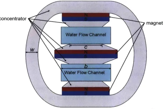
Validation

Firstly, the function of the inner concentrator and the loop is validated. Here, three cases are discussed about to validate the function of the inner concentrator and the

(41)

1.4 1.2 0.8 0.6 b e0.4 0.2 -- Demagnetization Curve -12 -10 -8 -6 -4 -2 0

Magnetic Field Intensity (A/m) x105

Figure 3-5: Demagnetization curve for N42 grade Neodymium magnets.

loop respectively. The first case is only the three-layer magnets, while the second one adds the inner concentrator, and the third one adds the loop. The material used for the concentrator here is mu-metal. And the loop width w is set to 0.005 m. The magnetic flux vector plot and y-directional magnetic flux density contour are shown

in Figure 3-6 and Figure 3-7 respectively.

(b) (c) B (T) 0.9 0.8 <.- 0.7 0.6 0.5 -0.3 0.2 0.1

Figure 3-6: Magnetic flux vector plot. (a) only magnets; (b) magnets and inner

(42)

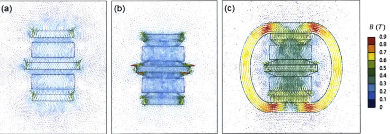
(a) By (T) 0.9 075 0.6 H0.45

Figure 3-7: Contour of magnetic flux density in y-direction. (a) only magnets; (b) magnets and inner concentrator;

(c)

magnets, inner concentrator, and loop with width w=0.005 m.

From the contour and the vector plot, it is clearly shown that the flux is guided

by the high-permeability material. And in Figure 3-6 (c), the loop collects almost all of the flux with opposite direction starting from the top side of the top magnet to the bottom side of the bottom magnet. And the magnetic flux density in the loop can even reach 0.9 T at the ends of the ellipses where the loop

just

collects most of the flux out of the magnets. And when the flux travels in the loop, some flux leaks into the surroundings. From the contour comparison, it is shown that with the inner concentrator and the loop, the directional magnetic flux density is greatly amplified. The average y-directional magnetic flux density By in the channel is also calculated, and shown in Table 3-2.

Table 3.2: Simulation results for effect validation. Case Number Case Description Average By Comments

1 Figure 3-6 (a) 0.156 T

2 Figure 3-6 (b) 0.176 T 12.8% more than case 1.

3 Figure 3-6 (c) 0.342 T 119.2% more than case 1.

The effect of the inner concentrator is limited by its size and it can also concentrate the flux with opposite direction. After adding the loop, flux with both directions are guided. And most of the flux with the undesired direction is constrained in the loop, thus the Average B is dramatically amplified.

(43)

Material

The effect of the concentrator highly depends on the magnetic permeability of the ma-terial. The concentrator role is to attract more flux within this material to rearrange the magnetic flux distribution. But this effect may be also limited by other proper-ties, such as the induction saturation, which constrains the maximum flux density in the concentrator.

The two typical materials discussed here are mu-metal and Metglas 2417A, whose B-H curves are shwon in Figure 3-8. Metglas has a much higher permeability, but lower saturation induction at only 0.6 T.

0.8 0.8

(a) 0.-.- -- Mn-metal (b 8--e-Mu-metal

0.7 A -Metg 0.7 - A -M 0.6 . ---- A - - - -A -- -- 0.6 ----. --- -0.5 05 0.4 0.4 0.2- 2 0.2-0.1 0.1 0 0 0 100 200 300 400 500 0 5 10 15 20

MagneticFieldIntensity (A/rn) MagneticFieldIntensity (A/m)

Figure 3-8: B-H curve of mu-metal and Metglas. (a) overview; (b) detailed view.

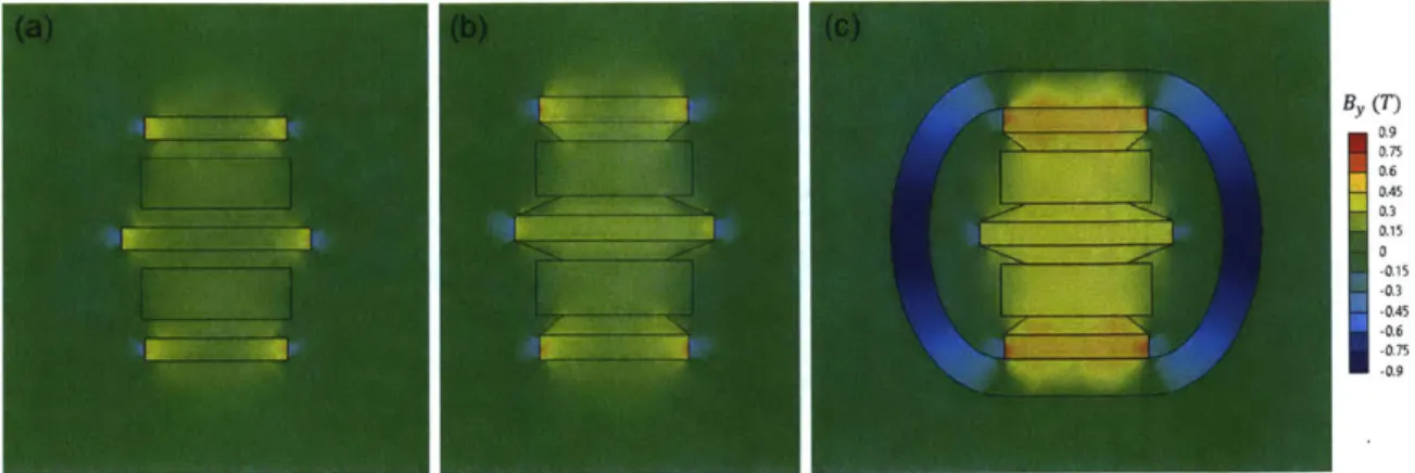
The contour of magnetic flux density in y-direction, magnetic flux vector plot, and the contour of magnetic flux density magnitude of the cases with 5 mm loop width are shown in Figure 3-9, Figure 3-10, and Figure 3-11, respectively.

In Figure 3-9, the contour of the two cases are almost the same, except for that, with mu-metal concentrators, By is stronger in the area of magnets. The average By

in the channel are calculated to be 0.329 T and 0.342 T for the Metglas concentrator and the mu-metal concentrator.

In Figure 3-10 and Figure 3-11, the magnetic flux density in the loop of mu-metal is much higher than that in the Metglas loop. And thus more flux with opposite direction is constrained by the mu-metal loop, resulting in a higher magnetic flux

(44)

(a)

Figure 3-9: Contour of magnetic flux density in y-direction. metal. By (n 0.9 0.75 0.6 0.45 0.3 0.15 0 -0.15 -0.3 -0.45 -0.6 -0.75 -0.9

(a) metglas; (b)

mu-B(T) 0.9 0.8 0.7 0.6 0.5 0.4 0.3 0.2 0.1 0

Figure 3-10: Magnetic flux vector plot. (a) metglas; (b) mu-metal.

density in the water channel. The similar difference between the materials happens almost in all different loop widths. The average By in the channel is 0.249 T and

0.255 T for Metglas and mu-metal at loop width of 0.002 m, while 0.417 T and 0.422

T for Metglas and mu-metal at loop width of 0.015 m.

Thus the saturation induction of the concentrator material is the key property

(a) (.)

6

(45)

-I B (T) 09 0.8 0.7 0.6 OA 0.3 0.2 0

Figure 3-11: Contour of magnetic flux density magnitude. (a) metglas; (b) mu-metal.

in this concentrator design. Although Metglas owns a much higher magnetic perme-ability than mu-metal, it is still desirable to choose mu-metal because of its much higher induction saturation value. And in the following discussion, only material of mu-metal will be focused on.

Loop width

The loop width is another important parameter influencing the effect of the concen-trator, as it determines the max amount of flux the loop can contain and guide. To systematically discuss the effect of the loop width, a series of simulations are run with various loop widths from 1 mm to 15 mm. And the average By are calculated and plotted in Figure 3-12.

The average By increases with the loop width before 0.01 m, where the relationship is almost linear. In this period, the magnetic flux density in the material is saturated and thus the magnetic flux with opposite direction the material contains is linear with the loop width. When the loop width exceeds 0.01 m, the material induction saturation stops. Thus, it does not change with the loop width any more, as almost all the magnetic flux with opposite direction is constrained in the loop already. The

(46)

0.5 C, 0.45 0.4 0.35 0.3 0.25 0.2 1 1 1 0 0.002 0.004 0.006 0.008 0.01 0.012

Loop width w (m)

Figure 3-12: Average B. in the channel with various loop widths.

magnetic flux density contour of the case with loop width of 0.002 m, and 0.015 m are shown in Figure 3-13.

B (T)

0.9

OA

M 3

Figure 3-13: Magnetic flux density contour for the cases with loop size of (a) 0.002

m; (b) 0.015 m.

-A-Mu-metal without two magnets outside

A

0 Ao

AA

(47)

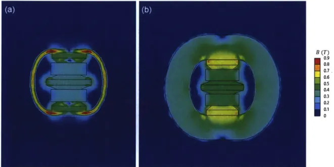
After comparing with Figure 3-11 (b) and Figure 3-13, it is found that the mag-netic flux density in the loop with the size of 0.002 m and 0.005m are almost the same, while the magnetic flux density of the 0.015 m width loop is much weaker. Thus the above anaylsis is validated. When determining the optimal loop size, simulations should be performed first and then the optimal loop width can be decided according to the results. Moreover, it's useless to further increase the loop size after the average By does not increase any more.

Magnets outside

It can be validated by the results in Section 3-2 that additional stronger magnets

placed outsides the pipe can strengthen the magnetic flux density in the channel. But the loop with high permeability can make a difference on this results because the loop may contain and block the flux generated by the strong magnets. This effect can occupy part of the material capability to guide the opposite flux density from the three-layer magnet.

In this part, the loop width changes from 1 mm to 12 mm, where 12 mm is the max loop size we can place in this setting. And the material selected in the simulations is mu-metal with the B-H curves shown in Figure 3-8. The average By in the channel of these cases are plotted in Figure 3-14.

At small loop widths, the two strong magnets outside can help build a stronger magnetic flux density field. But when the loop width exceeds 0.008 m, the effect of the two magnets outside can even reduce the magnetic flux density.

From the vector plot with 0.01 m width loop, it is clearly shown that with the two big magnets, the loop uses too much of its capability to contain and guide the flux generated by the big magnets. And thus more flux with opposite direction generated

by the three-layer magnet is distributed in the water channel, resulting in a weaker

magnetic flux density within the flow channel. After removing the big magnets, the mangetic flux density increases from 0.408 T to 0.422 T by 3.4%. Moreover, the existence of the two strong magnets generates magnetic field everywhere in the space, which may cause severe noise and damage to the sensors along the pipe.

(48)

0.5 C) 0.45 0.4 F-0.35 F 0.3 0.25 F 0.2 ' 1 0 0.002 0.004 0.006 0.008 0.01 0.012 Loop width w (m)

Figure 3-14: Average By in the channel with and without two big magnets outside.

(T) 0.8 0.7. 0.6 0.5 0.4 0.3 0.2 0.1 0

Figure 3-15: Magnetic flux vector with and without two big magnets outside.

Thus, a 0.01 m width loop with only the three-layer magnet is the best results in the analysis of this part. With pipes and magnets of other sizes, similar analysis can be conducted and then the optimal parameters can be determined.

- -Mu-metal without two magnets outsi

-A-

Mu-metal with two magnets outside

& - -El-C

AA

(b) Tik I r C"

i

3

Design and optimization of an MHD energy harvester for intelligent pipe systems

Design and Optimization of an MHD Energy

Harvester for Intelligent Pipe Systems

by

Xiaotong Zhang

Submitted to the Department of Mechanical Engineering

in partial fulfillment of the requirements for the degree of

Master of Science in Mechanical Engineering

at the

MASSACHUSETTS INSTITUTE OF TECHNOLOGY

June 2019

©

Massachusetts Institute of Technology 2019. All rights reserved.

Signature redacted

Department of Mechanical Engineering

May 17, 2019

CSignature

redacted

Kamal Youcef-Toumi

Professor

Thesis Supervisor

Signature redacted

...

.

. . . ....

.

Nicolas Hadjiconstantinou

Chairman, Committee on Graduate Students

JUN 13 2019

Design and Optimization of an MHD Energy Harvester for

Intelligent Pipe Systems

by

Xiaotong Zhang

Abstract

Acknowledgments

Contents

List of Figures

List of Tables

Chapter 1

Introduction

1.1

Background and Motivations

1.2

Previous Studies on Smart Pipe Systems

[4].

[5].

[6].

1.3

Previous Studies on Energy Harvesting

1.3.1

Turbine

1.3.2

Direct electromagnetic induction

1.3.3

Piezoelectric effect

1.3.4

Magnetohydrodynamics

[17].

[6],

1.4

Contribution and Thesis Outline

Chapter 2

MHD Energy Harvester Modelling

2.1

Generalized Ohm's Law

2.2

Power Extracted

+

2.3

Power Generated

2.4

Hall Effect

3

#

2.5

Discussion

2.6

Summary

Chapter 3

Magnetic Field Analysis and