HAL Id: hal-00943401
https://hal.archives-ouvertes.fr/hal-00943401
Submitted on 12 Feb 2014
HAL is a multi-disciplinary open access
archive for the deposit and dissemination of
sci-entific research documents, whether they are
pub-lished or not. The documents may come from
teaching and research institutions in France or
abroad, or from public or private research centers.
L’archive ouverte pluridisciplinaire HAL, est
destinée au dépôt et à la diffusion de documents
scientifiques de niveau recherche, publiés ou non,
émanant des établissements d’enseignement et de
recherche français ou étrangers, des laboratoires
publics ou privés.
A compiled Cycle Accurate Simulation for Hardware
Architecture
Adrien Bullich, Mikaël Briday, Jean-Luc Béchennec, Yvon Trinquet
To cite this version:
Adrien Bullich, Mikaël Briday, Jean-Luc Béchennec, Yvon Trinquet. A compiled Cycle Accurate
Simulation for Hardware Architecture. 5th International Conference on Advances in System SimSimulation
-SIMUL 2013, Oct 2013, VENICE, Italy. pp.213-225. �hal-00943401�
ComCAS: A Compiled Cycle Accurate Simulation
for Hardware Architecture
Adrien Bullich, Mika¨el Briday, Jean-Luc B´echennec and Yvon Trinquet
IRCCyN - UMR CNRS 6597 1, rue de la No¨e 44 321 Nantes Cedex 3 France
Email: {first name.last name}@irccyn.ec-nantes.fr
Abstract—The context of our research works is the real-time embedded systems domain. It is often difficult to test systems in order to ensure an appropriate running. A simulator presents the advantage that the detailed evolution of each component can be followed. These simulators require a very long development time. HARMLESShas been developed to automate this step. It is a hardware description language (HADL), readable by a compiler which allows the generation of a functional simulator (ISS) and a temporal simulator (CAS). CAS are costful in execution time. Several techniques exist in the literature to improve the speed of temporal simulators. In this paper we explore a new approach: the compiled simulation, which is used for functional simulators.
I. INTRODUCTION
Our works are in the field of real-time embedded systems. Since this kind of systems becomes more and more employed and complex, the guarantee of a correct running is an important property. We need to validate the security (the system disallows dangerous behaviours) of the system. Three different methods exist to give these results: the model-checking in the first step of the development, the simulation and series of tests in the last step. These different methods give complementary results. For example, the simulation allows to examine the evolution of each component in an operating system, whereas it is a difficult thing with series of tests in embedded systems. In this paper, our approach focuses on simulation techniques.
Several kinds of simulators are in the literature, according to the field studied, objectives followed or the abstraction level required. For hardware simulation, the implementation is complex, costful in time, and errors are difficult to avoid. That is the reason why people would rather use simulator generators. The construction of a simulator generator is based on a Hardware Architecture Description Language (HADL).
We can make out functional simulators i.e. Instruction Set Simulator (ISS), and temporal simulators i.e. Cycle Accurate Simulator (CAS). The simulation of real-time systems needs temporal informations, so we consider especially CAS. This kind of simulators has the disadvantage to be costful in execu-tion time. In this paper, we propose to explore a technique to improve the speed of CAS: ComCAS, a compiled simulation for CAS. Our works are in the context of simulation based on the HARMLESSlanguage, which implements an ISS and a CAS with interpreted methods [1].
The paper is organized in seven parts: this introduction, related works, the interpreted model, the compiled model,
valuation of the model size, performances and finally prospects for future works.
II. RELATED WORKS
Several kinds of simulators based on HADL are in the literature. For a simulation about the functional aspect, an Instruction Set Simulator (ISS) is required (nML [2], ISDL [3], HARMLESS [4] for example). It gives the instructions behaviour, without considering the details of the microarchitec-ture. If temporal informations are expected, a Cycle Accurate Simulator (CAS) is required (LISA [5], MADL [6], HARM
-LESS[7] for example). In this case, the microarchitecture must be modeled.
Compiled simulation, opposed to interpreted simulation, is a general programming technique in order to speed the execution of a simulator. It consists in moving certain tasks from the execution to the compilation. In an interpreted sim-ulator, these tasks are done during the execution and, in a compiled simulator, they are done during the compilation. In consequence, compiled simulation has shorter execution time than interpreted simulation, but longer compilation time. Since compilation is done less times than execution (classicaly, one compilation for several executions), it could be a global gain of time.
An ISS can be implemented like an interpreted simulator or a compiled simulator [8]. In that case, the task moved from the execution to the compilation is the analysis of the program to simulate. In spite of having a faster simulator, this leads to have a less flexible one: the compiled simulator is attached to a particular program, and if a user wishes to simulate a new one, he needs to compile again.
For ISS, compiled simulation uses Binary Translation (BT) ([9] or [10]). It consists of translating the binary program in order to be executed on the simulator operating system.
In the context of real-time systems, CAS is more appropri-ate, because it allows temporal considerations. Nevertheless, the implementation is more complex and it is a costful ap-proach, considering the execution time. Few methods exist to lighten this execution time.
In the literature, we mainly find interpreted methods (HARMLESS for example [7]). The technique of BT cannot easily be adapted to CAS, but solutions exist [11], coupling interpreted parts and translated parts. We also finds statistic approaches, called Cycle Approximate Simulator, based on
the sampling of instructions [12]. However it is not exactly equivalent with a CAS, because of margin of errors.
In the state of our knowledge, the technique of compiled simulation has not yet been employed to speed CAS, because of restrictions it implies: it is difficult to determine statically the evolution of the microarchitecture, especially because of indirect branches or self-modifying code. It is, however, the main contribution of the paper.
III. INTERPRETED SIMULATION MODEL
The contribution of the compiled simulation must be as-sessed in comparison with the interpreted approach associated. In this section, we present the interpreted model of the HARM
-LESS-based simulator [1], who is the base of our ComCAS model.
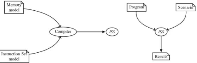
CAS are mainly implemented thanks to interpreted meth-ods, it is based on the interpretation of the code during the execution. The construction of a CAS includes the construction of an ISS, in order to get functional aspects of the system. The modelisation of an ISS requires the modelisation of the instruction set and of the memory. We globally obtain the development chain presented in figure 1.
The development of a CAS requires precedent elements and the modelisation of the microarchitecture which has a great influence on the temporal evolution of the system, and especially the pipeline architecture who determines the management of data hazards, structure hazards and control hazards. In figure 2, we get the development chain of a CAS.
Memory model
Instruction Set model
Compiler ISS ISS
Scenario
Results Program
Fig. 1. The development of an ISS requires the modelisation of the instruction set and the memory
Memory model Microarchitecture model Instruction Set model
Compiler CAS CAS Scenario
Results Program
Fig. 2. The development of a CAS requires the modelisation of the instruction set, the memory and the microarchitecture
In [1], the authors use the model of finite automata, because the system can be considered as a discrete transition one (an evolution at each cycle). That is the definition on which our contribution is based. A state represents the system in a particular cycle. To determine it, we need informations on the microarchitecture. This is given by:
• which instruction is in each stage of the pipeline
• and the state of internal resources.
Internal resources are elements of the microarchitecture, whose availability allows or not the evolution of an instruction in the pipeline. Stages of the pipeline are considered as internal resources.
A transition represents a discrete event who brings the system from a state to another. It is determined by the state of external resources and the instruction who may enter in the pipeline.
External resources are elements who are not in the mi-croarchitecture, but whose avaibility has an influence on the evolution of an instruction in the pipeline. It is the case of memory for example. As they are external of our modelisation, their avaibility is determined during the execution by the intervention of external resources.
In order to lighten the model, the authors use instruction classes (instructions with same behaviours) and not directly instructions.
The content of states is abstracted, and informations re-quired for the simulation are gathered on transitions. That is why transitions are labeled with notifications (answering if a particular event happens or not).
We can now formalize the model as it follows.
Let AI an automaton defined by {S, s0, ER, IC, N, T }, where:
• S is the set of states,
• s0 is the initial state (empty pipeline) in S,
• ER is the first alphabet of actions (external resources), • IC is the second alphabet of actions (instructions
class),
• N is the alphabet of labels (notifications),
• T is the transition function in S × ER × IC × N × S.
[____] [b___] [_b__] [a_b_] 0:b(0) 0:a(0) 1:a(0) 1:b(0) 0:b(1) 0:a(1) 1:a(1) 1:b(1) 0:a(0) 1:a(0) 0:b(0) 1:b(0) ... ... ... ...
Fig. 3. Automaton in interpreted simulation: 0:b(1) means that the external resource is free (0), that the instruction b may enter in the pipeline and that the notification happens (1)
In the example of figure 3, the notation [b_a_] represents the state of the pipeline: it means that instruction b is in the first stage and instruction a is in the third stage. There are no others instructions.
We have only one notification who represents the entry of an instruction in the second stage of the pipeline. There are one
external resource. The instruction b needs to take the external resource to enter in the pipeline.
We note 01:a(10) a transition (in T) where 01 ∈ ER means that the first external resource is taken (1) and the second is free (0), a ∈ IC means that an instruction of class a enters in the pipeline, 10 ∈ N means that the first notification does not happen (0) and the second does (1).
The run of the automaton is done throught the intermediary of external resources and the instruction class. It means that the simulator computes the new state of external resources and the new instruction class in order to fire a transition and to find the new state in the automaton. Firing the transition, we get the state of notifications. They give informations to the user about the performing of the simulation. They are helpful to compute the new state of external resources too.
IV. COMCASMODEL
In this section, we adapt the interpreted model to be a compiled one: the ComCAS model.
The compiled simulation is opposed to the interpreted simulation according to the repartition of tasks between compi-lation and execution. We recall that, in our case, the task is the analysis of the program. An interpreted simulator analyzes the program during the execution. A compiled simulator analyzes the program during the compilation.
Because of this moving, the compiled simulation has a faster execution than the interpreted simulation. However, the compiled simulation has an heavier compilation time than the interpreted simulation. This is not necessarily a problem: usu-ally, the compilation is done only one time and the execution several times.
A compiled simulation is compiled for a special architec-ture and for a special program. Consequently, the simulator is less flexible, attached to a particular program. If the need is to simulate several programs, the interpreted simulation will be more efficient. But if the need is to simulate only one program with different scenarios, the compiled simulation will be more efficient.
In the figure 2 and 4 we can see the difference between the development chain of the interpreted simulation and the compiled simulation (respectively). We notice especially that for the interpreted simulation the program is at the end of the development chain, at the beginning for the compiled simulation.
To perform the interpreted model to a compiled model, we need to add informations on the program reading in the system, i.e. the PC and the memory of called function. Then, the determination of our system is given by:
• which instruction is in each stage of the pipeline, • the state of internal resources,
• the position in the program reading (the Program Counter)
• and the memory of called functions (a stack of Pro-gram Counter in order to return in previous functions).
Memory model Microarchitecture model Instruction Set model Program
Compiler ComCAS ComCAS Scenario
Results
Fig. 4. The development of a compiled CAS requires to move the program analysis in the compilation
With this model, instructions become labels on the au-tomaton and no more actions. Indeed, we only determine the evolution of the system with external resources and instructions become an information we get of this run. We put on transi-tions the instruction to execute, as an event. However, it cannot be reduced to a simple notification (a boolean information), so we add the Program Counter (PC) on the transition label.
We can formalize our ComCAS model as it follows. Let AC an automaton defined by {S, s0, ER, I, N, T }, where:
• S is the set of states,
• s0is the initial state (empty pipeline, initial PC, empty stack) in S,
• ER is the alphabet of actions (external resources), • I is an alphabet of labels (instructions),
• N is an other alphabet of labels (notifications), • T is the transition function in S × ER × I × N × S.
[____] pc0 stack [a___] pc1 stack [_a__] pc1 stack [b_a_] pc2 stack 10:pc1(0) 00:pc1(0) 01:pc1(0) 11:pc1(0) 10:-(1) 00:pc2(1) 01:pc2(1) 11:-(1) 00:pc2(0) 01:pc2(0) 10:-(0) 11:-(0) ... ... ... ...
Fig. 5. Automaton in compiled simulation: 10:pc1(0) means that the first external resource is free and the second taken (10), that the instruction with PC pc1 enters in the pipeline and that the notification does not happen (0)
In the example of figure 5, we have only one notification who represents the entry of an instruction in the second stage of the pipeline. There are two external resources. The instruction b, with PC pc2, needs to take the second external resource to enter in the pipeline.
We note 10:pc1(0) a transition (in T) where 10 ∈ ER means that the first external resource is free (0) and the second taken (1), pc1 ∈ I means that the instruction with PC pc1
enters in the pipeline, 0 ∈ N means that the first notification does not happen (0).
The management of branches uses a specific external re-source. If this resource is taken, we consider the branch taken. If it is not, we consider the branch is not taken. During the simulation, we can detect jump in PC and define dynamically the value of this resource. In order to represent the latency of the branching, according to the branching policy, an other spe-cific external resource could be employed and simulate control hazards. If the microarchitecture uses branching predictor, the simulator would emulate this branching predictor and define dynamically the value of the correponding external resource. While the resource is defined to be taken, the following instruction could not enter in the pipeline.
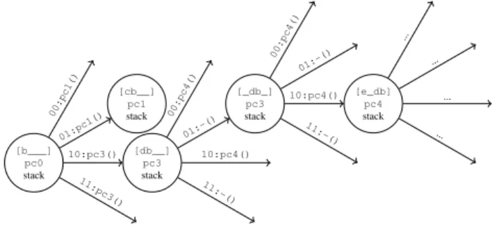
An example is given in figure 6. The first external resource represents the branch to pc3. If it is taken, then the model goes to pc3, else it goes to the next PC pc1. The second resource represents the branching latency. As long as it is taken, no instruction cannot enter in the pipeline.
[b___] pc0 stack [cb__] pc1 stack [db__] pc3 stack [_db_] pc3 stack [e_db] pc4 stack 00:pc1() 01:pc1() 10:pc3() 11:pc3() 00:pc4() 01:-() 10:pc4() 11:-() 00:pc4() 01:-() 10:pc4() 11:-() ... ... ... ...
Fig. 6. The second external resource specifies if the branch b is taken or not. The first external resource specifies if the instruction e can enter or not in the pipeline.
The compiled simulation needs to compute statically the control flow of the program in order to model it during the compilation. In the case of indirect branches or code self-modifying, this computation is impossible unless we execute the different scenarios of the program. That is the main restriction of our model. Without the possibility to determine statically the target of indirect branches, the solution is to plan the different possibilities. Unfortunately, it leads to a considerable increase of the size of the automaton.
Indirect branches are unavoidable if we want to model functions calls, because of RETURN instructions. For this specific problem, a PC stack is added in states. The stack in states allows to memorise original PC when is executed a CALL instruction. When a RETURN instruction is executed, thanks to this stack, it is possible to determine the target PC of the branch, during the compilation.
The processus is the following. When a CALL instruction enters in the pipeline, we push the original PC in the stack and we branch to the target PC. When a RETURN instruction enters in the pipeline, we pop a PC from the stack and we branch on it. An example is given in figure 7.
The main advantage of the compiled simulation is to make possible the move of analysis functions in the compilation step. For example, the interpreted method manages data hazards during the execution, thanks to the intervention of an external
pipeline PCcall [] pipeline PCk [PCcall] pipeline PCreturn [pccall] pipeline PCcall+1 []
Fig. 7. A CALL function push the original PC in the stack, and a RETURN function pop the PC from the stack
resource. It is a task costful in time. In our model, we compute statically the data dependency, verifying if instructions in the critic section of the pipeline do not write in registers we want to read. This technique solves data hazards directly during the compilation.
V. VALUATION OF THE NUMBER OF STATES
In order to give an idea of the complexity of ComCAS model, we propose to valuate the number of states.
A state is composed of the pipeline state, the PC read and the stack of called functions. In a first step, we will consider there are no stack in states, and we will add their consideration in the last step. The global method consists in counting pipeline states for a PC given. We find three different situations in the control flow: linear configuration, beginning of the program and branching configuration.
In a linear configuration, for a PC given, one past exists. Consequently, the state of the pipeline is only determined by stalls. The problem is reduced to a combinatory one: if s is the number of stages, we count Ck
s (k among s) pipeline states with k instructions inside (k ∈ [0; s]). Thus, the total number of pipeline states is Psk=0Csk.
If the PC read is at the beginning of the program, pcnwith n < s, it is impossible to put more than n instructions in the pipeline. So, in this case, the previous value is truncated to Pn
k=0C k
s. To simplify calculus, we use fs: n → Pn
k=0C k s. And we know that fs(s) = 2s.
At this step of our computation, we can valuate the number of states in a perfect linear program (with no branch). Let i the number of instructions. The s first instructions are in the second case (beginning of the program), and i − s others instructions are in the first case (endless linear configuration). It gives: Ps−1k=0fs(k) + (i − s).2s. This value is a maximum and it is reached if every pipeline states are explored. It is the case if an external resource manages the entry of instructions in the first stage, allowing all stalls arrangements.
To count pipeline states is more complex if we include branches in the control flow. Let us consider the case in figure 8, with k < s. In this situation, if we put j instructions in the pipeline with j ≤ k, the branching is not visible in the pipeline. Thus, we remain in the same previous situation: Csj pipeline states. But, if we put j instructions in the pipeline with j > k, then for each stalls arrangement two pipeline states exist, with the two different origins. So we count 2.Csjpipeline states. The total number of pipeline states is Pkj=0Cj
s+ Ps j=k+12.C j s. It is equivalent with 2s+1− fs(k).
For one branching situation, we have k varying in [0; s−1]. Let b the number of branch targets. So the total number of states becomes Ps−1k=0fs(k) + (i − s − s.b).2s+ b.(s.2s+1− Ps−1
pcn−k−1 pc0n−k−1
pcn−k
pcn−1
pcn
Fig. 8. A branch configuration in the control flow. If k < s then in PC pcn
the pipeline can remember two origins.
(1 − b). s−1 X k=0
fs(k) + (i − (1 − b).s).2s
The expression is valid if branch configuration is the same we give in figure 8. It means two conditions:
• branch targets are separated by more than s instruc-tions,
• no branch less than s instructions after a branch target. In fact, we can confirm that the first condition does not degrade our valuation. The second condition is more important and avoid too small loops.
The analysis of our valuation reveals that the number of states is linear with the number of instructions, and exponential with the number of stages. We can compare the expression with the number of states in interpreted simulation: (ic + 1)s, which is more exponential considering s.
In our valuation, we have not yet considered the use of PC stack in states. We can see in figure 9 the effect on the control flow of the add of PC stacks.
pc0 pccall pc2 pccall0 pc4 pc5 pck pcret pc0[] pccall[] pc2[] pccall0[] pc4[] pc5[] pck[pccall] pcret[pccall] pck[pccall0 ] pcret[pccall0 ]
Fig. 9. Stack consideration consists in an inline in the control flow. These two automata are equivalent.
It can be regarded as inlining: functions are duplicated. If we consider this new control flow, our reasoning is the same. Let us call i0the number of couple of instruction and PC stack, and b0 the new number of branch targets. Thus, the number of states becomes: (1 − b0). s−1 X k=0 fs(k) + (i0− (1 − b0).s).2s
The influence of this inlining is very dependent on the code. For example, we observe that programs using floating numbers increase significantly the size of the automaton, and make the building of the model difficult.
VI. TESTS ANDPERFORMANCES
In this section, we present experimental results about performances of ComCAS model in comparison with the interpreted simulation.
The architecture simulated in these tests is a PowerPC (MPC 5516, a RISC architecture from Freescale). We simulate benchmarks of M¨alardalen [13]. Simulations are made with an Intel Core i7 vpro computer. We execute 50 000 times each program.
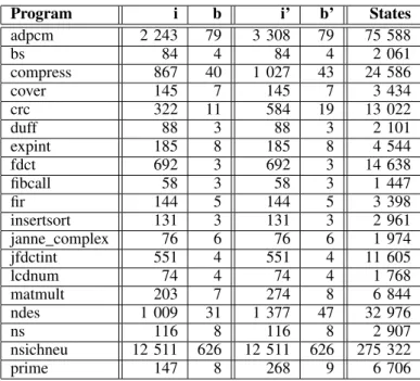
We give in figure 10 an illustration of the influence of the inlining and the number of states. This allows to confirm that if a function is called one time during the execution, PC stack has no influence on the size of the model. We note that the number of states is smaller than the valuation we give, because the model does not explore every pipeline states. With particular external resources (making every pipeline states possible) we get the same result than our valuation. To allow a comparison, with the same configuration the interpreted model gets 1 024 states. Smaller is the code, smaller is our model.
Program i b i’ b’ States adpcm 2 243 79 3 308 79 75 588 bs 84 4 84 4 2 061 compress 867 40 1 027 43 24 586 cover 145 7 145 7 3 434 crc 322 11 584 19 13 022 duff 88 3 88 3 2 101 expint 185 8 185 8 4 544 fdct 692 3 692 3 14 638 fibcall 58 3 58 3 1 447 fir 144 5 144 5 3 398 insertsort 131 3 131 3 2 961 janne complex 76 6 76 6 1 974 jfdctint 551 4 551 4 11 605 lcdnum 74 4 74 4 1 768 matmult 203 7 274 8 6 844 ndes 1 009 31 1 377 47 32 976 ns 116 8 116 8 2 907 nsichneu 12 511 626 12 511 626 275 322 prime 147 8 268 9 6 706
Fig. 10. Influence of the inlining: i is the number of instructions, b the number of branch targets, i’ the number of instructions with the inlining and b’ the number of branch targets with the inlining
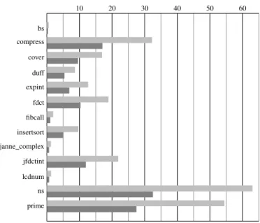
The figure 11 represents performances of ComCAS model in comparison with the interpreted method for the execution time. The compilation in the compiled approach is more com-plex than the interpreted approach. It contains: construction
of the ISS, analysis of the program (thanks to the ISS), construction of the model and final compilation.
As we said before, benefits in execution time is paid with heavier compilation step. This drawback can be easily coun-terbalanced if several execution are done for a compilation.
10 20 30 40 50 60 bs compress cover duff expint fdct fibcall insertsort janne complex jfdctint lcdnum ns prime
Fig. 11. Comparison of execution time in s. Gray is for interpreted simulation and black is for compiled simulation.
The main impact of our model comes from the possibil-ity of managing during the compilation analysis tasks and especially the data dependency control. In the interpreted simulation, during the execution, the functionality tasked with data dependency management, costs correctly 30% of the total time, explaining the benefit we get.
VII. PROSPECTS
In this paper, we have discussed of the different techniques to implement high speed Cycle Accurate Simulator. We study the difference between interpreted simulation and compiled simulation in the implementation of Instruction Set Simulator. We develop a model to adapt this compiled approach to Cycle Accurate Simulator: ComCAS. We study the theoritical size of our model. Finally, we compare performances of our model with the interpreted method associated.
It appears to bring efficiency because it allows the remove of analysis tasks in the execution step. However, the technique is limited by the use of indirect branches, else the size of the automaton could increase considerably. Nevertheless, we make possible to take in consideration CALL and RETURN instructions, in order to simulate classical programs.
In the future, we propose to work on a Just In Time Simulator, which could bring a solution to the problem of indirect branches.
Then, we propose to improve the efficiency of the ComCAS model thanks to the move in the compilation step of the fetch cache management and thanks to a reduction of states, using ”macro-instructions”. In a compiled simulation it is possible to consider gathering of instructions to reduce the automaton and the execution time.
REFERENCES
[1] R. Kassem, M. Briday, J.-L. B´echennec, G. Savaton, and Y. Trinquet, “HARMLESS, a hardware architecture description language dedicated to real-time embedded system simulation,” Journal of Systems Architecture - doi: http://dx.doi.org/10.1016/j.sysarc.2012.05.001, 2011.
[2] A. Fauth, J. Van Praet, and M. Freericks, “Describing instruction set processors using nml,” EDTC’95: Proceedings of the 1995 European Conference on Design and Test, p. 503, 1995.
[3] G. Hadjiyiannis, S. Hanono, and S. Devadas, “Isdl: an instruction set description language for retargetability,” DAC’97: Proceedings of the 34th annual conference on Design automation, pp. 299–302, 1997. [4] R. Kassem, M. Briday, J.-L. B´echennec, Y. Trinquet, and G. Savaton,
“Instruction set simulator generation using HARMLESS, a new hardware architecture description language,” Simutools ’09: Proceedings of the 2nd International Conference on Simulation Tools and Techniques, 2009.
[5] S. Pees, A. Hoffmann, V. Zivojnovic, and H. Meyr, “Lisa - machine description language for cycle-accurate models of programmable dsp architectures,” DAC’99: Proceedings of the 36th ACM/IEEE conference on design automation, pp. 933–938, 1999.
[6] W. Qin, S. Rajagopalan, and S. Malik, “A formal concurrency model based architecture description language for synthesis of software devel-opment tools,” in Conference on Languages, Compilers, and Tools for Embedded Systems (LCTES’04), 2004.
[7] R. Kassem, M. Briday, J.-L. B´echennec, G. Savaton, and Y. Trinquet, “Simulator generation using an automaton based pipeline model for timing analysis,” in International Multiconference on Computer Science and Information Technology (IMCSIT’08), Wisla, Poland, October 2008. [8] C. Mills, S. C. Ahalt, and J. E. Fowler, “Compiled instruction set simulation,” Software - Practice and Experience, vol. 21, pp. 877–889, 1991.
[9] C. Cifuentes and V. Malhotra, “Binary translation: Static, dynamic, retargetable?” Proceedings International Conference on Software Main-tenance, pp. 340–349, 1996.
[10] F. Bellard, “Qemu, a fast and portable dynamic translator,” Translator, vol. 394, pp. 41–46, 2005. [Online]. Available: http://www.usenix.org/ event/usenix05/tech/freenix/full papers/bellard/bellard html/
[11] D. Jones and N. Topham, “High speed cpu simulation using ltu dynamic binary translation,” Proceedings of the 4th International Conference on High Performance and Embedded Architectures and Compilers, 2009. [12] R. E. Wunderlich, T. F. Wenisch, B. Falsafi, and J. C. Hoe, “Smarts: Accelerating microarchitecture simulation via rigorous statistical sam-pling,” Proceedings of the 30th annual international symposium on Computer architecture, pp. 84–97, 2003.
[13] J. Gustafsson, A. Betts, A. Ermedahl, and B. Lisper, “The M¨alardalen WCET benchmarks – past, present and future,” B. Lisper, Ed. Brussels, Belgium: OCG, Jul. 2010, pp. 137–147.