HAL Id: hal-00343805
https://hal.archives-ouvertes.fr/hal-00343805
Submitted on 3 Dec 2008
HAL is a multi-disciplinary open access
archive for the deposit and dissemination of
sci-entific research documents, whether they are
pub-lished or not. The documents may come from
teaching and research institutions in France or
abroad, or from public or private research centers.
L’archive ouverte pluridisciplinaire HAL, est
destinée au dépôt et à la diffusion de documents
scientifiques de niveau recherche, publiés ou non,
émanant des établissements d’enseignement et de
recherche français ou étrangers, des laboratoires
publics ou privés.
On The Performance of Human Visual System Based
Image Quality Assessment Metric Using Wavelet
Domain
Alexandre Ninassi, Olivier Le Meur, Patrick Le Callet, Dominique Barba
To cite this version:
Alexandre Ninassi, Olivier Le Meur, Patrick Le Callet, Dominique Barba. On The Performance of
Hu-man Visual System Based Image Quality Assessment Metric Using Wavelet Domain. SPIE Conference
Human Vision and Electronic Imaging XIII, Jan 2008, San Jose, United States. pp.680610.1-680610.12.
�hal-00343805�
On The Performance of Human Visual System Based Image
Quality Assessment Metric Using Wavelet Domain
A. Ninassi
a,b, O. Le Meur
a, P. Le Callet
band D. Barba
ba
Thomson Corporate Research, 1 Avenue Belle Fontaine 35511 Cesson-Sevigne, France;
b
IRCCyN UMR 6597 CNRS, Ecole Polytechnique de l’Universite de Nantes
rue Christian Pauc, La Chantrerie 44306 Nantes, France
ABSTRACT
Most of the efficient objective image or video quality metrics are based on properties and models of the Human Visual System (HVS). This paper is dealing with two major drawbacks related to HVS properties used in such metrics applied in the DWT domain : subband decomposition and masking effect. The multi-channel behavior of the HVS can be emulated applying a perceptual subband decomposition. Ideally, this can be performed in the Fourier domain but it requires too much computation cost for many applications. Spatial transform such as DWT is a good alternative to reduce computation effort but the correspondence between the perceptual subbands and the usual wavelet ones is not straightforward. Advantages and limitations of the DWT are discussed, and compared with models based on a DFT. Visual masking is a sensitive issue. Several models exist in literature. Simplest models can only predict visibility threshold for very simple cue while for natural images one should consider more complex approaches such as entropy masking. The main issue relies on finding a revealing measure of the surround influences and an adaptation: should we use the spatial activity, the entropy, the type of texture, etc.? In this paper, different visual masking models using DWT are discussed and compared.
Keywords: Quality Assessment, Human Visual System, DWT, DFT, Contrast Masking, Entropy Masking
1. INTRODUCTION
The aim of an objective image quality assessment is to create an automatic algorithm that evaluates the picture or video quality as a human observer would do. Image quality assessment has been extensively studied during this past few decades and many different objective criteria have been built. The quality metrics based on models of the Human Visual System (HVS) are an important part of the different approaches in image quality assessment. HVS models may be classified into mono-channel or multi-channel models. This work focus on the latter. In order to simulate the multi-channel behavior of the HVS and to well qualify the visual masking effects, this kind of quality metrics rests on a perceptual subband decomposition. This decomposition is often realized in the frequency domain like Fourier domain. The use of Fourier domain leads to good performances, but with high computational complexity. One solution to deal with this would be to use a spatial transform like a wavelet transform. Nevertheless, the correspondence between the visual system and the wavelet domain is known to be only approximate1.2 This issue results in non-optimal visual performance, especially in the setting up of the visual masking. But even if the visual masking effects are non-optimal, what is the decrease in performance in terms of quality assessment?
In this paper, the performances loss between an image quality metric using Fourier domain and an image quality metric using wavelet domain are evaluated. An efficient image quality metric based on a multi-channel model of the HVS using wavelet domain is described. This metric provides quality scores well correlated with those given by human observers. The HVS model of the low-level perception used in this metric includes subband decomposition, spatial frequency sensitivity, contrast masking and entropy masking.
The subband decomposition of this multi-channel approach is based on a spatial frequency dependent wavelet transform. Advantages and limitations of the wavelet transform as a part of a HVS model are discussed, and compared with a HVS model based on a Fourier transform. The spatial frequency sensitivity of the HVS is simulated by a wavelet contrast sensitivity function (CSF) derived from Daly’s CSF.3 Masking effects include both contrast masking and entropy masking. Entropy masking allows to consider the modification of the visibility
threshold due to the semi-local complexity of an image. In this work, the impact of entropy masking on image quality assessment is also evaluated both quantitatively and qualitatively. Like many quality metrics in the literature, the proposed metric is implemented in two stages. In the first stage, the visibility of the errors between the original and the distorted image is locally evaluated resulting in a perceptual distortion map. In the second stage, a spatial pooling combines the distortion map values into a single quality score.
In order to investigate its efficiency, the wavelet based quality assessment (WQA) metric is compared with subjective ratings and two objective methods. The first is a Fourier based quality assessment metric (FQA). The second objective method is the state-of-the-art measure of structural similarity (SSIM).4 The WQA metric is tested with and without entropy masking, giving insight into the relevance of the entropy masking.
This paper is organized as follows. In the section 2, advantages and limitations of the DWT are discussed, and compared with models based on DFT. Section 3 is devoted to the description of the WQA metric. The WQA and FQA approaches are compared, as well as the different masking functions in section 4. Finally, general conclusions are provided.
2. DWT/DTF IN HVS MODELS : ADVANTAGES AND LIMITATIONS
The visual masking effect is a key feature of the HVS, whereby an image signal can be masked, i.e. its visibility reduced, by another image signal. This phenomenon is strongest when both signals appear in approximately the same spatial location, with approximately the same spatial frequency, and orientation. These observations are due to the multi-channel structure of the HVS, and have led to the development of multi-channel models of the HVS. In the literature, several subband decompositions were used to simulate the multi-channel behavior of the HVS like the cortex transform,5 or the Perceptual Subband Decomposition (PSD).6The PSD, illustrated Figure 1(a), has been characterized with psychovisual experiments and is defined by analytic filters in the Fourier domain. So its similarity degree with the HVS is high, but its computational complexity is high.
1.5 cy/d° 5.7 cy/d° 14.2 cy/d ° 28.2 cy/d ° L F II II I IV fy (cy/d°) fx (cy/d°) (a) Image Fmax (cy/d°) HH1 HL1 HH1 HH1 HH1 HL1 LH1 LH1 HH2 HL2 HH2 HH2 HH2 HL1 LH2 LH2 HH3 HL3 HH3 HH3 HH3 HL3 LH3 LH3 LF (b)
Figure 1. (a) Perceptual subband decomposition (PSD). (b) Spatial frequency dependent DWT. DWT LF and PSD LF mapping (L=4).
Spatial transform such as DWT is a good alternative to reduce computation effort but the correspondence between the perceptual subbands and the usual wavelet ones is not straightforward. The DWT has similarities with the multi-channel models of the HVS. In particular, both decompose the image into a number of spatial frequency channels that respond to an explicit spatial location, a limited band frequencies, and a limited range of orientations. However, significant differences exist between DWT and PSD.
First, PSD is non-separable and non-dyadic, whereas DWT is separable and dyadic. The orientation and the frequency ranges of the DWT subbands are different of the PSD ones. For the luminance, the angular selectivity of the PSD is 45˚or 30˚according to the radial frequency channel. The angular selectivity of the DWT is only
45˚and the diagonal band contains mixed orientations of 45˚and -45˚. This is a problem with masking because the energy near 45˚does not not significantly mask energy near -45˚, and interference between them are able to occur. For the luminance, the frequency ranges of the PSD are 0 cy/d˚to 1.5 cy/d˚, 1.5 cy/d˚to 5.7 cy/d˚, 5.7 cy/d˚to 14.2 cy/d˚and 14.2 cy/d˚to 28.2 cy/d˚. The frequency ranges of the DWT depends both of the maximum spatial frequency fmax of the image (i.e. the visualization conditions), and the subband level. The level-dependent frequency ranges are [2−(l+1)fmax; 2−lfmax] where l is the subband level (l = 0 corresponds to the highest frequencies). The number of decomposition levels impacts the discrepancy between the frequency ranges of the DWT and the frequency ranges of the PSD.
Another problem is the shape of the DWT filters. Horizontal and vertical bands encroach on diagonal frequencies. The energy of diagonal edge can end up in the horizontal and vertical bands. If edge contrast is high enough, the amplitudes of the coefficients related to the edge into the horizontal and vertical bands may be high enough so that the resulting masking effect can be overestimated. Furthermore, the energy displaced away from the diagonal band into the horizontal and vertical bands will be energy that is not taken into account in the masking of diagonal structures.
3. QUALITY METRIC DESCRIPTION : WQA
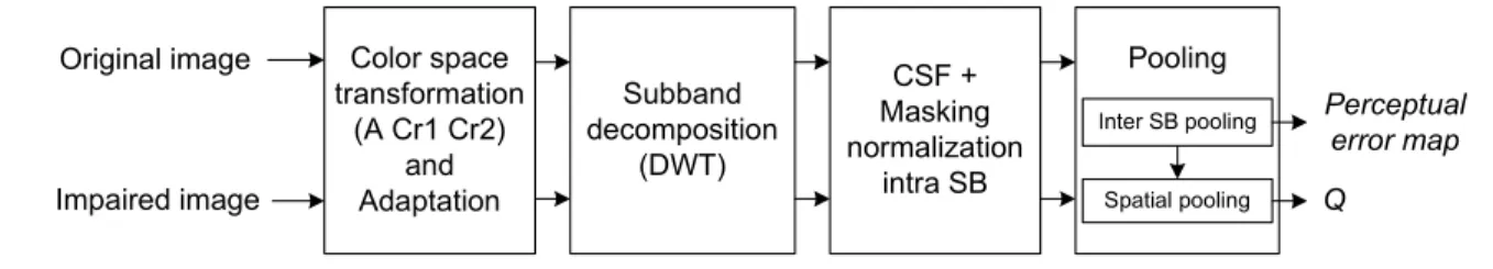
In this section the wavelet based quality assessment method (WQA) is described. Figure 2 illustrates the structure of the WQA. As mentioned before, the HVS model of the low level perception used in this metric includes subband decomposition, spatial frequency sensitivity, contrast masking and entropy masking.
The quality assessment method based on the Fourier domain (FQA) used in this work is inspired from the metric proposed in,7 except for the error pooling stage. The WQA model is similar to FQA model, except for the subband decomposition. Moreover, in the FQA model, the masking functions were limited to the Daly’s derived ones. The versions of WQA and FQA used in this work are achromatic versions. The luminance component used in these metrics is defined as the cardinal direction A of the opponent color space defined by Krauskopf.8 The first step is the same for both FQA and WQA. This step consists of color space transformation and adaptation. Adaptation describes the changes that occur due to different illumination levels in the visual sensibility of lightness. Subband decomposition (DWT) CSF + Masking normalization intra SB Pooling Original image Perceptual error map Impaired image Color space transformation (A Cr1 Cr2) and
Adaptation Spatial pooling
Inter SB pooling
Q
Figure 2. Structure of the WQA
3.1 Subband decomposition
In the FQA model, a PSD was used. This type of decomposition is achieved in the Fourier domain. This decomposition is the result of a number of studies conducted at the university of Nantes since 1990.6 Therefore, if only one advantage should be given, it will be its high similarity degree with the human visual system. As most of video sequences have a resolution that is not in power of two, the time needed both to apply the Fourier transform and to perform the subband decomposition is high. With this kind of approach, the real-time can not be easily reached. This is why it is necessary to re-think the design of the subband decomposition. More specifically, new subband decomposition, probably less biologically plausible but less complex, has to be proposed. A subband decomposition defined by wavelet filters is used and supposed to describe the different channels in the human vision system. This subband decomposition is based on a spatial frequency dependent wavelet transform approximating the PSD characterized in previous works,6and defined by analytic filters. The PSD is illustrated Figure 1(a). The Discrete Wavelet Transform (DWT) used is the CDF 9/7 (Cohen-Daubechies-Feauveau). The
number of decomposition levels L is chosen so that the low frequency (LF) DWT subband matches to the LF subband of the PSD (cf. Figure 1(b)).
3.2 Contrast sensibility function
The Contrast Sensibility Function (CSF) describes the variations in visual sensitivity as a function of spatial frequency and orientation. As complete frequency representation of the images is not available, the CSF is applied over the DWT subband. The wavelet coefficients cl,o(m, n) are normalized by the CSF using one value by DWT subband:
˜
cl,o(m, n) = cl,o(m, n) · Nl,oCSF, (1) For each subband a CSF value NCSF
l,o is calculated from the 2D CSF defined by Daly.3 This value is the mean of the 2D CSF over the covered frequency range for each subband. The CSF is normalized by its maximum prior to be integrated, so NCSF
l,o ∈ [0; 1].
3.3 Masking functions
Masking is a rather well known effect that refers to the changes of visibility increase (pedestal effect) or decrease (masking effect) of a signal due to the presence of background (masking signal).
Thanks to the subband decomposition, the visual masking stage allows the modeling of the visibility mod-ification. The visual masking effect concerns here both contrast masking and entropy masking. The former is used to take into account the modification of the visibility threshold due to the contrast value, whereas the latter allows to consider the modification of the visibility threshold due to the neighborhood characteristics. The term ’entropy masking’ was first used by Watson9 who argues that image quality models should incorporate entropy masking, as well as contrast masking. The entropy masking reflects the notion that the masking is a function of the degree to which the mask is unknow, i.e. the uncertainty of the masking signal. This phenomenon is also called activity masking, texture masking, or local texture masking.10 Due to the influence of the neighborhood characteristics, this masking effect will be called semi-Local Masking (sLM) in the rest of the paper.
Four Different masking functions were tested. The first two are adaptations of Daly’s masking model3 using or not the neighborhood. The last two are adaptations of Nadenau’s masking11 model using or not the neighborhood.
3.3.1 Contrast masking by using Daly’s model (Daly)
As proposed by Daly,3the visibility threshold elevation Tl,o(m, n) at site (m,n) in the subband (l,o), where l is the level and o is the orientation, is given by:
Tl,o(m, n) = (1 + (k1· (k2· |˜cl,o(m, n)|)s)b) 1 b k1, k2= constant Subband dependent : s ∈ [0.65; 1]; b ∈ [2; 4] , (2)
where ˜cl,o(m, n) is the CSF-normalized wavelet coefficient at site (m, n), k1 and k2determine the pivot point of the curve, and the parameter b determines how closely the curve follow the asymptote in the transition region. In the initial work of Daly, a value for the learning slope, describe by the Equation (2), is chosen depending on the subband (cortex subband). Ideally, this value should depend on the uncertainty of the signal masking. One way to deal with the semi-local masking is to locally adapted the slope s in function of the neighborhood activities.
3.3.2 Semi-Local masking by modifying Daly’s model (Daly sLM)
In3Daly has noted that the parameter s corresponds to the slope of the high masking contrast asymptote, which ranges between 0.65 and 1.0. For a high uncertainty (low learning level), the slope is 1.0 and as the learning
increases, the slope (and uncertainty) reduces to 0.65. The visibility threshold elevation Tl,o(m, n) at site (m, n) in the subband (l,o), where l is the level and o is the orientation, is given by:
Tl,o(m, n) = (1 + (k1· (k2· |˜cl,o(m, n)|)s(m,n))b) 1 b k1, k2= constant s(m, n) = S + ∆s(m, n) ∈ [0.65; 1] Subband dependent : b ∈ [2; 4]; S ∈ [0.65; 0.8]
∆s(m, n) : semi − local complexity ∈ [0; 1 − S]
, (3)
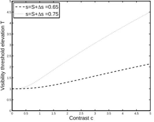
where the parameters are the same as in the Equation (2), except for parameter s(m, n) which depends on the neighborhood. The semi-local complexity parameter ∆s(m, n) is estimated from the component A of both the reference image and the impaired image. First the semi-local activity values of a n-by-n neighborhood are computed on the component A for both the reference image and the impaired image. Figure 3 illustrates the slope modification of the masking function due to the semi-local complexity parameter ∆s(m, n).
0 0.5 1 1.5 2 2.5 3 3.5 4 4.5 5 0 0.5 1 1.5 2 2.5 3 3.5 4 4.5 5 Contrast c
Visibility threshold elevation T
s=S+∆s =0.65
s=S+∆s =0.75
Figure 3. Slope modification of the masking function due to the semi-local complexity parameter ∆s(m, n)
The semi-local activity value is evaluated through the entropy on a n-by-n neighborhood. Entropy at site (m,n) is defined as :
E(m, n) = −Xp(m, n) · log(p(m, n)) , (4) where p(m,n) is the probability calculated from the luminance histogram of a n-by-n neighborhood around site (m,n), and E(m, n) is the resulting entropy map. Then, the entropy values E(m, n) are mapped to the ∆s(m, n) values respectively, through a sigmoid function :
∆s(m, n) = b1
1 + e−b2·(E(m,n)−b3) , (5) where b1, b2, b3 are empirically deduced (trial on various types of texture).
3.3.3 Nadenau : Intra-Channel Model (Nadenau)
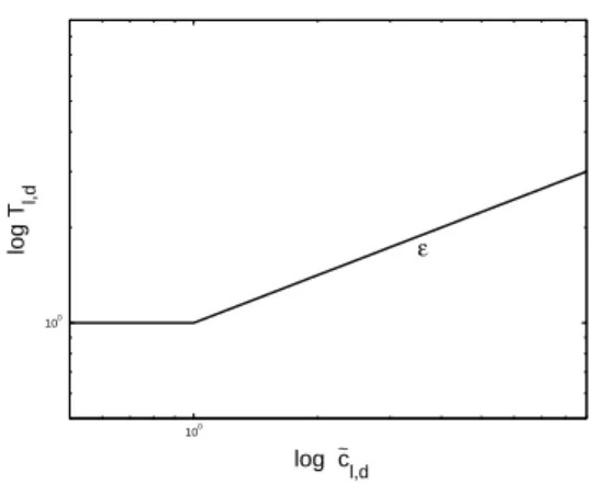
In his work11Nadenau proposed a simple intra-channel (IaC) contrast model applied on the wavelet coefficients. The non-linearity of the threshold elevation function is approximated by two piece-wise linear functions :
Tl,o(m, n) = max(1, ˜cl,o(m, n)ε) , (6) where ε is the slope-parameters. Figure 4 illustrates the shape of this curve.
100 100 log c~ l,d log T l,d ε
Figure 4. Threshold elevation function Teis characterized by slope-parameter ε
3.3.4 Nadenau : Intra-Channel Model with semi-Local Masking (Nadenau sLM)
In his work11 Nadenau proposed also an intra-channel contrast model applied on the wavelet coefficients and using the semi-local activity. This model is inspired from the so called extended masking12 in the framework of J2K. Basically, it considered the point-wise contrast masking as captured by the IaC-model, but applies additionally an inhibitory term that takes the neighborhood activity into account :
Tl,o(m, n) = max(1, ˜cl,o(m, n)ε) · (1 + ωΓ) . (7) where ωΓ is the correction term for the influence of an active or homogeneous neighborhood. It is the normalized sum of the neighboring coefficients that were taken to the power of ϑ :
ωΓ= 1 (kL)ϑNΓ X Γ |˜cl,o|ϑ. (8)
The parameter kL determines the dynamic range of ωΓ, while NΓ specifies the number of coefficient in the neighborhood Γ. Contrary to Nadenau’s work, the neighborhood Γ is not chosen causal in this study, but as in the section 3.3.2, an-by-n neighborhood around site (m,n) is used.
3.3.5 Masking normalization and perceptual errors
For each subband (l, o), the masking normalization is applied on the error between the CSF normalized wavelet coefficients of the reference image and the impaired image. It results in a perceptual error map V El,o(m, n) according to: V El,o(m, n) = |˜cRl,o(m, n) − ˜cIl,o(m, n)| max(TR l,o(m, n), T I l,o(m, n)) . (9) where ˜cR
l,o(m, n), ˜cIl,o(m, n) are the CSF-normalized wavelet coefficients at site (m, n) in the reference and the impaired image respectively , and TR
l,o(m, n), T I
l,o(m, n) are the threshold elevation at site (m, n) in the reference and the impaired image respectively.
3.4 Error pooling
The goal of this stage is to provide both a distortion map expressed in term of visibility, stemming from the wavelet subbands, and a quality score. The inter subband pooling is divided in three steps (orientation pooling, level pooling and spatial pooling). As the pooling stage is not the focus of this work, the solution chosen is rather simple. It consists in using different Minkowski summations for each pooling steps, as given by Equations (10), (11) and (12).
The orientation pooling is computed with a Minkowski summation according to : V El(m, n) = 1 3 X d (V El,o(m, n))βo !βo1 , ∀d ∈ [LH, HL, HH] . (10)
After this stage L + 1 perceptual error maps are available. This stage provides L perceptual error maps, where L is the number of decomposition levels. The additional perceptual error map is the one corresponding to LF. The level pooling is computed with a Minkowski summation according to :
V E(m, n) = 1 L L X l=0 (V El(m, n))βl !βl1 . (11)
This stage provides an unique perceptual error map. The spatial pooling is computed with a Minkowski sum-mation resulting in the quality score Q :
Q = 1 M.N M X m=1 N X n=1 (V E(m, n))βs !βs1 . (12)
where M and N are the height and the width of the image respectively.
4. RESULTS
4.1 Quantitative analysis : MOS/MOSp
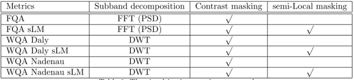
The performances of the different objective quality metrics presented in the previous section, and recapitulated in Table 1, are evaluated according to mean observer score (MOS).
MOS have been obtained by conducting subjective quality assessment experiments in normalized conditions (ITU-R BT 500-10). Images were displayed at a viewing distance of four times the height of the picture (80 cm), and their resolution was 512 × 512 pixels. The standardized method DSIS (Double Stimulus Impairment Scale) was used. Ten unimpaired pictures were used in these experiments. The pictures were impaired by JPEG, J2K compression or through a blurring filter scheme. One hundred and twenty impaired pictures are then obtained. Twenty unpaid subjects participated to the experiments. All had normal or corrected to normal vision. All were inexperienced observers (in video processing) and naive to the experiment.
Metrics Subband decomposition Contrast masking semi-Local masking
FQA FFT (PSD) √ FQA sLM FFT (PSD) √ √ WQA Daly DWT √ WQA Daly sLM DWT √ √ WQA Nadenau DWT √ WQA Nadenau sLM DWT √ √
Table 1. The six objective metrics compared
Prior to evaluate the objective image quality measures, a psychometric function is used to transform the objective quality score Q (cf. Equation (12)) in predicted MOS (MOSp), as recommended by the Video Quality Expert Group13(VQEG). The psychometric function is given by:
M OSp(Q) = b1 0
1 + e−b20·(Q−b30), (13)
The objective quality metrics are evaluated by comparing the MOS and the MOSp using three performance metrics recommended by VQEG. The three performance metrics are the linear correlation coefficient (CC), the Spearman rank order correlation coefficient (SROCC) and the root-mean-square-error (RMSE).
Results, presented in Tables 2, 3 and 4, and in Figures 7, 8, are reported for the different methods on the entire dataset as well as on individual datasets. The individual datasets are the images impaired by JPEG compression, the images impaired by J2K compression , the images impaired by compression (JPEG+J2K), and the images impaired by a blurring filter scheme. For information and to allow readers to make their own opinions on the image dataset, PSNR and SSIM4 are also evaluated on the entire dataset (cf. Table 2).
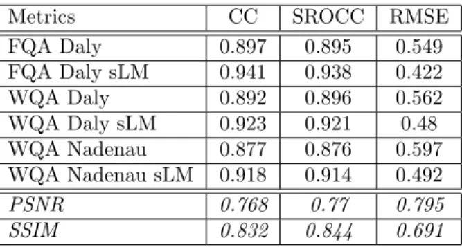
Metrics CC SROCC RMSE FQA Daly 0.897 0.895 0.549 FQA Daly sLM 0.941 0.938 0.422 WQA Daly 0.892 0.896 0.562 WQA Daly sLM 0.923 0.921 0.48 WQA Nadenau 0.877 0.876 0.597 WQA Nadenau sLM 0.918 0.914 0.492 PSNR 0.768 0.77 0.795 SSIM 0.832 0.844 0.691
Table 2. Results on the entire dataset
Results on the entire dataset are presented in Table 2. The six multi-channel models (FQA and WQA) outperform SSIM and PNSR, in terms of CC, SROCC and RMSE. ∆CC between the multi-channel models and the SSIM goes from +0.045 to +0.109. It is not surprising since SSIM do not simulated the multi-channel structure of the HVS. FQA without sLM model outperforms, all version of the WQA without sLM, in terms of CC and RMSE. ∆CC between the FQA without sLM model and WQA without sLM models goes from +0.005 to +0.02. In the same way FQA with sLM model outperforms all version of the WQA with sLM, in terms of CC, SROCC and RMSE. ∆CC between the FQA with sLM model and WQA with sLM models goes from +0.018 to +0.023. These observations show that FQA models are always better than WQA models, which illustrated the fact that the PSD better simulated the multi-channel behavior of the HVS than the frequency dependent wavelet transform. The results on the individual dataset J2K presented in Table 3 lead to the same conclusion. However, the results on the JPEG dataset, JPEG+J2K and Blur dataset, presented in Tables 3 and 4 are quite different. On the JPEG and JPEG+J2K datasets, FQA model without sLM outperforms WQA models without sLM, but FQA with sLM is outperformed by WQA Daly with sLM. On the Blur dataset WQA models without sLM outperform FQA models without sLM which is quite surprising. Furthermore, the WQA Daly with sLM is outperformed by the other models with sLM. The superiority of the FQA models is observed on the entire dataset, even if their performances depend on the type of impairment.
JPEG J2K
Metrics CC SROCC RMSE CC SROCC RMSE FQA Daly 0.857 0.862 0.599 0.936 0.947 0.457 FQA Daly sLM 0.938 0.939 0.403 0.947 0.952 0.414 WQA Daly 0.851 0.854 0.611 0.906 0.916 0.549 WQA Daly sLM 0.96 0.965 0.327 0.94 0.946 0.439 WQA Nadenau 0.821 0.823 0.665 0.908 0.917 0.542 WQA Nadenau sLM 0.916 0.915 0.467 0.947 0.948 0.415
Table 3. Results on the JPEG dataset and J2K dataset
The use of the semi-local masking in the three different configurations (FQA Daly vs FQA Daly sLM, WQA Daly vs WQA Daly sLM, and WQA Nadenau vs WQA Nadenau sLM) consistently increases the performance of the model in terms of CC, SROCC and RMSE. This observation is done on the entire dataset, as well as on the JPEG dataset, the J2K dataset and the JPEG+J2K dataset. On the entire dataset ∆CC between with and without sLM are respectively +0.044, +0.031 and +0.041 with FQA Daly, WQA Daly and WQA Nadenau.
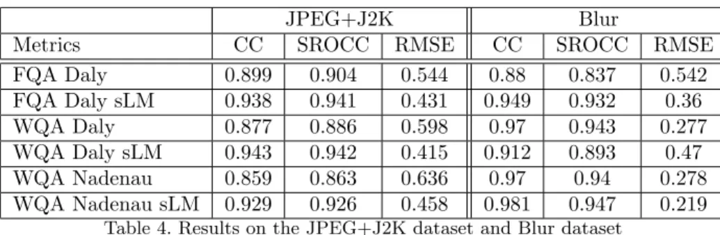
JPEG+J2K Blur
Metrics CC SROCC RMSE CC SROCC RMSE FQA Daly 0.899 0.904 0.544 0.88 0.837 0.542 FQA Daly sLM 0.938 0.941 0.431 0.949 0.932 0.36 WQA Daly 0.877 0.886 0.598 0.97 0.943 0.277 WQA Daly sLM 0.943 0.942 0.415 0.912 0.893 0.47 WQA Nadenau 0.859 0.863 0.636 0.97 0.94 0.278 WQA Nadenau sLM 0.929 0.926 0.458 0.981 0.947 0.219
Table 4. Results on the JPEG+J2K dataset and Blur dataset
The same trend is observed in terms of SROCC and RMSE. Results are more moderate on the Blur dataset, where the improvement is significant with the FQA Daly model, lower with WQA Nadenau model, and becomes a worsening with the WQA Daly model. A possible explanation lies in way that semi-local activity is taken into account. The blur impairments lead to a significant reduction of the semi-local activity between the reference image and the impaired image. As the error is normalized by the maximal threshold elevation between the reference image and the impaired image (cf. Equation (9)), the semi-local masking effect can be overestimated in this case. Theses observations show the positive impact of the semi-local masking, and prove that the masking effect must not be limited to contrast masking.
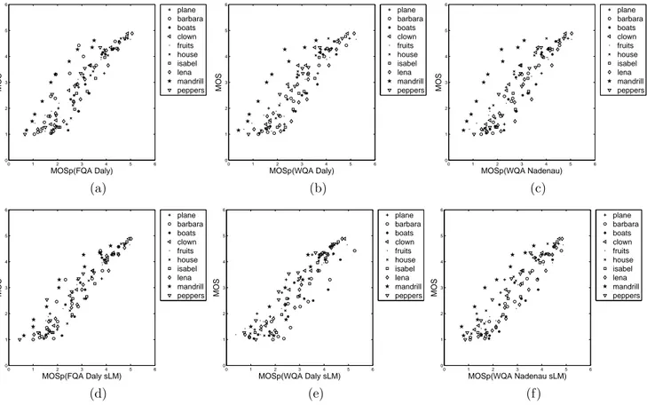
Figures 7 and 8 plot MOS according to MOSp. Figure 7 allows to analyze the impact of the semi-local masking on the different types of impairment. The improvement due to the semi-local masking is not specific to one particular type of impairment. Whatever the type of impairment, the semi-local masking brings a significant improvement. Figure 8 allows to analyze the impact of the semi-local masking on the different contents (impaired images from the same reference image). Figure 8 shows that the improvement due to the semi-local masking is more specific to the images noted I, which arise from the same reference image : Mandrill (cf. Figure 5(a)). The content of these images is particular because of their large texture areas (beards and moustaches). The quality of these images is underestimated by the models without sLM, or in other words, the distortions are overestimated. The use of the semi-local masking improves significantly the quality evaluation of these images. This observation tends to show that the overestimated distortions are located in the areas with important spatial activity. It means that semi-local masking plays important part in these areas.
4.2 Qualitative analysis (semi-Local Masking)
(a) (b) (c) (d)
Figure 5. (a) is Mandrill ,(b) is Mandrill with JPEG compression, (c) and (d) are WQA perceptual error maps with Daly masking and with Daly sLM masking respectively
Figure 5(a,b) represents the original image Mandrill and a JPEG compressed version of Mandrill respectively. The difference between the perceptual error map of the WQA Daly model (cf. Figure 5(b)), and the perceptual error map of WQA Daly sLM (cf. Figure 5(c)) is significant. The masking effect in the most active areas like the beard areas, is underestimated with the WQA Daly model, but it is closer to the reality with WQA Daly sLM model. This observation is to be linked to the one done in the previous section. The fact that image Mandrill
is the most impacted by the semi-local masking is probably due to both the coverage ratio of the texture areas, and the type of the textures.
(a) (b) (c) (d)
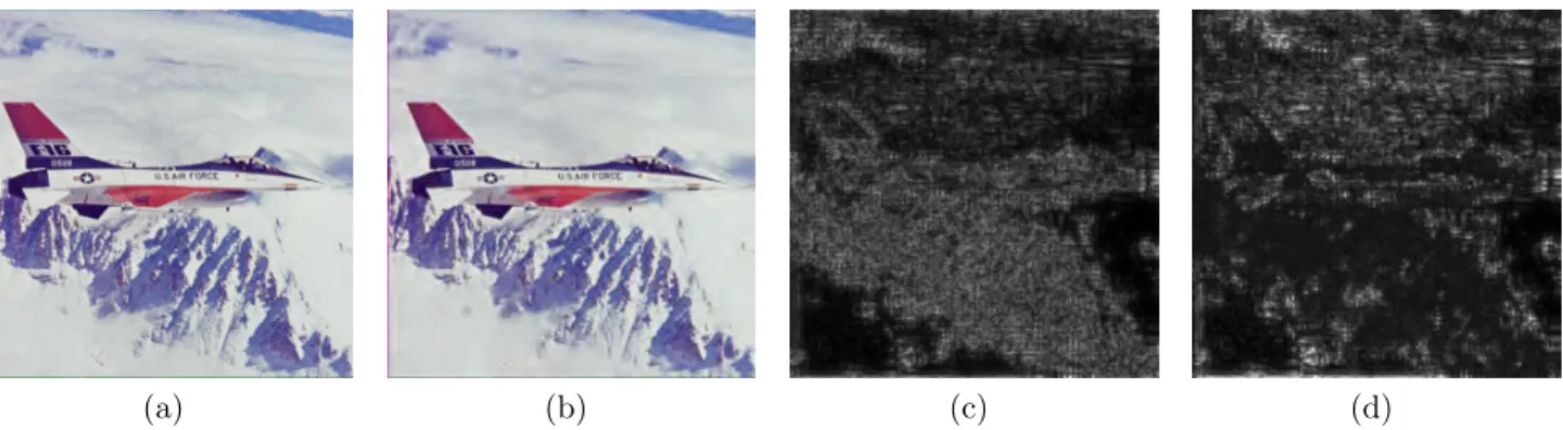
Figure 6. (a) is Plane ,(b) is Plane with J2K compression, (c) and (d) are WQA perceptual error maps with Daly masking and with Daly sLM masking respectively
Figure 6(a,b) represents the original image Plane and a J2K compressed version of Plane respectively. The difference between the perceptual error map of the WQA Daly model (cf. Figure 6(b)), and the perceptual error map of WQA Daly sLM (cf. Figure 6(c)) is also significant. The masking effect in the most active areas like the mountains, is underestimated with the WQA Daly model, but it is closer to the perception with WQA Daly sLM model. However, the masking effect is overestimated on specific areas like the strong edges around the tail of the plane, or like the lettering on the plane. This is due to the semi-local activity measure. The entropy is a good estimator of the semi-local activity but it tends to overestimate the semi-local activity in the neighborhood of strong edges with high contrast. A semi-local activity measure based on variance would lead to the same default.
5. CONCLUSION
Firstly, this paper has shown that doing a PSD in the Fourier domain, or doing a subband decomposition using DWT to simulate the multi-channel structure of the HVS does not lead to same performance. As expected the Fourier based models outperforms the wavelet based models. However the wavelet based models still have good prediction performance. A spatial transform such as DWT can be considered as a good alternative to reduce computation effort.
Secondly, the positive impact of the semi-local masking on some images is important and complementary to contrast masking. Integration of this type of masking in quality metrics improves both the prediction performance of the metrics, and the relevance of their perceptual error maps. The semi-local entropy measure leads to good results, even if it tends to overestimate the masking effect on the neighborhood of strong edges with high contrast. Future work includes further investigation to find more revealing measures of the surround influences on masking effect. In particular the measures must be able to avoid an overestimation of the masking effect on the neighborhood of strong edges with high contrast. Furthermore, more studies have to be done on the way to take into account the semi-local masking when there are strong differences between the semi-local activity of the reference image and the semi-local activity of the impaired image.
REFERENCES
1. W. Zeng, S. Daly, and S. Lei, “An overview of the visual optimization tools in JPEG2000,” Signal Processing: Image Communication 17(1), pp. 85–104, 2002.
2. A. P. Bradley, “A wavelet visible difference predictor,” IEEE Transactions on Image Processing 8(5), pp. 717–730, 1999.
3. S. Daly, “The visible differences predictor : an algorithm for the assessment of image fidelity,” Proc. SPIE 1666, pp. 2–15, 1992.
4. Z. Wang, A. C. Bovik, H. R. Sheikh, and E. P. Simoncelli, “Image quality assessment: From error visibility to structural similarity,” IEEE Trans. on Image Processing 13, pp. 600–612, 2004.
5. A. B. Watson, “The cortex transform : Rapid computation of simulated neural images,” Comput. Vis., Graph., Image Process. 39, pp. 311–327, 1987.
6. H. Senane, A. Saadane, and D. Barba, “The computation of visual bandwidths and their impact in image decomposition and coding,” International Conference and signal Processing Applications and Technology , pp. 766–770, 1993.
7. P. Le Callet and D. Barba, “A robust quality metric for color image quality assessment,” International Conference on Image Processing 1, pp. 437–440, 2003.
8. D. R. Williams, J. Krauskopf, and D. W. Heeley, “Cardinal directions of color space,” Vision Research 22, pp. 1123–1131, 1982.
9. A. B. Watson, R. Borthwick, and M. Taylor, “Image quality and entropy masking,” in Human Vision, Visual Processing, and Digital Display VIII, 3016, (San Jose, CA, USA), 1997.
10. M. D. Gaubatz, D. M. Chandler, and S. S. Hemami, “Spatial quantization via local texture masking,” Proc. SPIE Human Vision and Electronic Imaging X. 5666, pp. 95–106, 2005.
11. M. Nadenau, Integration of Human Color Vision Models into High Quality Image Compression. PhD thesis, ´
Ecole Polytechnique F´ed´erale de Lausanne, 2000.
12. S. Daly, W. Zeng, and S. Lei, “Visual masking in wavelet compression for JPEG2000,” Proc. SPIE Image and Video Communications and Processing 3974, 2000.
13. VQEG, “Final report from the video quality experts group on the validation of objective models of video quality assessment,” March 2000. http://www.vqeg.org/.
0 1 2 3 4 5 6 0 1 2 3 4 5 6 MOSp(FQA Daly) MOS JPEG J2K Blur (a) 0 1 2 3 4 5 6 0 1 2 3 4 5 6 MOSp(WQA Daly) MOS JPEG J2K Blur (b) 0 1 2 3 4 5 6 0 1 2 3 4 5 6 MOSp(WQA Nadenau) MOS JPEG J2K Blur (c) 0 1 2 3 4 5 6 0 1 2 3 4 5 6 MOSp(FQA Daly sLM) MOS JPEG J2K Blur (d) 0 1 2 3 4 5 6 0 1 2 3 4 5 6 MOSp(WQA Daly sLM) MOS JPEG J2K Blur (e) 0 1 2 3 4 5 6 0 1 2 3 4 5 6 MOSp(WQA Nadenau sLM) MOS JPEG J2K Blur (f)
Figure 7. MOS according to MOSp by degradations: (a), (d) are FQA Daly and FQA Daly sLM respectively; (b), (e) are WQA Daly and WQA Daly sLM respectively; (c), (f) are WQA Nadenau and WQA Nadenau sLM respectively
0 1 2 3 4 5 6 0 1 2 3 4 5 6 MOSp(FQA Daly) MOS plane barbara boats clown fruits house isabel lena mandrill peppers (a) 0 1 2 3 4 5 6 0 1 2 3 4 5 6 MOSp(WQA Daly) MOS plane barbara boats clown fruits house isabel lena mandrill peppers (b) 0 1 2 3 4 5 6 0 1 2 3 4 5 6 MOSp(WQA Nadenau) MOS plane barbara boats clown fruits house isabel lena mandrill peppers (c) 0 1 2 3 4 5 6 0 1 2 3 4 5 6 MOSp(FQA Daly sLM) MOS plane barbara boats clown fruits house isabel lena mandrill peppers (d) 0 1 2 3 4 5 6 0 1 2 3 4 5 6 MOSp(WQA Daly sLM) MOS plane barbara boats clown fruits house isabel lena mandrill peppers (e) 0 1 2 3 4 5 6 0 1 2 3 4 5 6 MOSp(WQA Nadenau sLM) MOS plane barbara boats clown fruits house isabel lena mandrill peppers (f)
Figure 8. MOS according to MOSp by reference image: (a), (d) are FQA Daly and FQA Daly sLM respectively; (b), (e) are WQA Daly and WQA Daly sLM respectively; (c), (f) are WQA Nadenau and WQA Nadenau sLM respectively