Publisher’s version / Version de l'éditeur:
Soil Dynamics and Earthquake Engineering, 9, 2, pp. 85-95, 1990
READ THESE TERMS AND CONDITIONS CAREFULLY BEFORE USING THIS WEBSITE. https://nrc-publications.canada.ca/eng/copyright
Vous avez des questions? Nous pouvons vous aider. Pour communiquer directement avec un auteur, consultez la première page de la revue dans laquelle son article a été publié afin de trouver ses coordonnées. Si vous n’arrivez pas à les repérer, communiquez avec nous à [email protected].
Questions? Contact the NRC Publications Archive team at
[email protected]. If you wish to email the authors directly, please see the first page of the publication for their contact information.
NRC Publications Archive
Archives des publications du CNRC
This publication could be one of several versions: author’s original, accepted manuscript or the publisher’s version. / La version de cette publication peut être l’une des suivantes : la version prépublication de l’auteur, la version acceptée du manuscrit ou la version de l’éditeur.
Access and use of this website and the material on it are subject to the Terms and Conditions set forth at
Silent boundary for time domain wave motion analyses based on direct
energy deletion
Hunaidi, O.; Towhata, I.; Ishihara, K.
https://publications-cnrc.canada.ca/fra/droits
L’accès à ce site Web et l’utilisation de son contenu sont assujettis aux conditions présentées dans le site LISEZ CES CONDITIONS ATTENTIVEMENT AVANT D’UTILISER CE SITE WEB.
NRC Publications Record / Notice d'Archives des publications de CNRC:
https://nrc-publications.canada.ca/eng/view/object/?id=303554c3-5316-42d0-8647-eebb2f64a68a https://publications-cnrc.canada.ca/fra/voir/objet/?id=303554c3-5316-42d0-8647-eebb2f64a68aSer
PHI
National Research
Conseil national
8
2
1
d1
+
1
Council Canada
da recharches Canada
no,
1647
c. 2
Institute for
lnstitut de
RLDG
Research in
recherche en
- -- -
Construction
construction
Reprinted from
Journal of Soil Dynamics and Earthquake Engineering
Vol. 9, No. 2, 1990
p. 85-95
(IRC Paper No. 1647)
I
Silent Boundary for Time Domain Wave
b
Motion Analyses Based on Direct Energy
Deletion
by M.O. Al-Hunaidi, 1. Towhata and K. lshihara
Canad8
Les auteurs proposent une nouvelle mCthode spCcialisCe pennettant de simuler la condition
de radiation des domaines non bornCs. Cette mkthode, dite <<de
type local,,, s'applique aux
modkles finis semi-discrets analyses dans le domaine temporel, compte tenu du
comportement Clastique linCaire de 1'extCrieur du domaine non borne et du comportement
non linCaire arbitraire de I'intCrieur.
La mCthode proposCe repose sur l'effacement de
1'Cnergie des ondes dans une rCgion limite Ctendue de sorte que le front des ondes rCflCchies
soit constamrnent empkhC de revenir
B
lfint6rieur du modkle fini. On utilise B cette
fin
une
proc&ux-e numirique simple qui entretient un champ d'ondes continu qui peut Etre trait6 par
le systkme discret sans crCer d'ondes de choc numeriques. I1 s'est aver6 que la prCcision de
la mCthode est fonction de la taille de la region lirnite Ctendue; plus la r6gion limite est
grande, plus la mCthode est p k i s e .
Silent boundary for time domain wave motion
analyses based on direct energy deletion
M. 0. Al-Hunaidi
Institute for Research in Construction, National Research Council of Canada, Ottawa, Ontario, Canada, K I A OR6 (formerly Graduate Student, University of Tokyo, Bunkyo-Ku, Tokyo, Japan)
I. Towhata and K. Ishihara
Department of Civil Engineering, University of Tokyo, Bunkyo-Ku, Tokyo, Japan
A new specialized method to simulate the radiation condition of unbounded domains is developed. This method is of the so called 'local type' and it is designed for semi-discretized finite models analysed in the time domain, considering linear elastic behaviour of the exterior unbounded domain and arbitrary nonlinear behaviour of the interior. The principle of the proposed method is based on erasing the wave energy in an extended boundary region so that the front of reflected waves is continually held back from the interior of the finite model. This is achieved via a simple numerical scheme which maintains a wave field continuity that can be handled by the discretized system without creating numerical wave shocks. It has turned out that the accuracy of the method is a function of the size of the extended boundary region; the larger the boundary region, the better the accuracy.
Key Words: dynamic analysis, finite element method, infinite media, vibration, wave propagation
1. INTRODUCTION truncated unbounded domain, (ii) determination of the
In recent decades, the emergence of computer simulation as a powerful solution tool has enabled engineers to analyze complex problems whose solutions are analyti- cally intractable, experimentally expensive or impossible. In spite of rapid upgrading of computer resources and decline in its cost, computational expense of complex engineering problems remains substantial. This is often the case for problems involving wave propagation in semi-infinite continua analysed in the time domain. In order to reduce the cost of analysing these problems, the computational model is restricted to a finite domain that contains geometrical and material irregularities. The remaining unbounded domain is truncated. Conse- quently, it is necessary to devise special boundary techniques to incorporate the radiation condition of the truncated unbounded domain into the finite computa- tional model. Otherwise, spurious wave reflections take place at the artificial boundaries of the model making the analyses unreliable. Artificial boundaries that satisfy the radiation condition are referred to in the literature as nonreflecting, absorbing, silent or transmitting boundaries. Silent boundary conditions can be classified into: (i) nonlocal conditions, and (ii) local conditions. Nonlocal boundaries are perfect absorbers, but their computational expense in time domain analyses is substantial as they involve the following' : (i) determining of the frequency dependent dynamic stiffness matrix of the
dynamic stiffness matrix in the time domain using inverse Fourier transform, and (iii) performing global con- volution integrals, in space and time, to evaluate the boundary force contribution of the missing unbounded domain. On the contrary, local boundary conditions, in space and time, are much less expensive to use, but they are disadvantaged by their approximate nature.
Several silent boundaries have been proposed for analyses performed in the frequency d ~ m a i n ~ - ~ . The so called consistent transmitting b ~ u n d a r y ~ , ~ is well known for its excellent accuracy and it is widely used for analysis of layered media. Analysis in the frequency domain is efficient for linear soil problems (i.e. under small strain). For soils with nonlinear characteristics, however, one has to resort to equivalent linear procedures. These procedures are not very reliable for the calculation of residual displacements which may be used as a failure criteria of soils supporting man-made structures. Therefore, the analysis in the frequency domain is not useful when soil properties have to be analysed in the time domain in which the time change of soil properties can be traced accurately.
Several silent boundaries for analysis in the time domain have been proposed and implemented with varying degrees of a c c ~ r a c y ~ - ' ~ . The viscous boundary
7-10 is very popular due to its implicity and low
computational cost. The shortcoming of this technique, however, is that viscous boundary conditions designed to
absorb body waves may not work well for ~ a ~ l e i ~ h
Paper accepted April 1988. Discussion ends August 1990. surface waves. Viscous boundary conditions that can
Silent boundary for time domain wave motion analyses based on direct energy deletion: M . 0. Al-Hunaidi et al.
properly absorb Rayleigh waves are a function of depth from the halfspace surface as well as the frequency of the incident wave.
In principle, a silent boundary condition is achieved if it is possible to predict the motion of the boundary nodes one time step ahead of the last time station. The predicted motion of the boundary nodes is, in turn, used to compute the force contribution from the truncated infinite domain. Few techniques of this type have been proposedl1.l2 in which the motion of boundary nodes is extrapolated from the motion of nodes in the vicinity of the boundary.
The superposition boundary is an elegant scheme to eliminate boundary reflectionst3. In this method, the reflections at a single boundary are cancelled by superimposing two solutions performed with free and fixed boundary conditions. In these solutions, in and out of phase reflections occur. Hence, addition of these two cases eliminates reflections. The improved version of this boundary14 reduces the computational expense substantially.
The paraxial boundary is a technique in which the usual equations of wave propagation in a small zone beside the boundary are replaced by paraxial wave equations which only allow wave propagation in one direction. A propagation in the opposite direction (reflected wave) is mathematically impossible1
'.
Application of this bound- ary scheme to finite element models requires some special numerical techniques to ensure smooth wave propagation from the interior elastic region of the model to the paraxial boundary domain16.An alternative approach to silent boundaries is the use of a very large finite element model in which a travelling wave decays with distance due to internal viscosity. This is achieved by increasing the size of viscous elements gradually with distance17. A variation of this idea is a transformation of coordinates by which the finite real elements are reduced to an equivalencet8 of finite size.
This paper introduces a new wave absorbing boundary of the local type that can be used in conjunction with semi-discretized systems analysed in the time domain. In the proposed wave absorption mechanism, the radiation condition at infinity is represented by directly deleting the wave energy through a special numerical scheme in a small region beside the boundaries of the finite model so that the front of reflected waves is continually prevented from propagating back into the interior of the model.
The effectiveness of the proposed boundary is demonstrated by two plane strain elasticity examples: (i) vertical load pulse on halfspace and (ii) Rayleigh wave example. Comparisons are made with two other silent boundaries; the standard viscous7 and the second order paraxial approximation16 boundaries. In these tests, finite elements are used to discretize the continuum, but finite differences can be used as well.
2. A NEW WAVE ABSORPTION MECHANISM The most reliable solution to avoid spurious wave reflections at artificial boundaries in a finite computa- tional model is to place these boundaries at a sufficient distance from the source of excitation; i.e. increasing the size of the model. This approach serves the purpose of delaying the arrival time of reflected waves to a zone of interest in the finite model until the required solution is obtained. However, it is disadvantaged by large storage requirements and high computational cost.
-
DELETE
_
BOUNDARY
I
Fig. I . Schematic view of direct wave deletion
In contrast, the remedy under consideration in this section is based on the novel approach of continually holding back the front of reflected waves from the interior of the model by numerical means instead of the above approach of locating the boundaries of the finite model at far distances. This aim is achieved by directly deleting wave energy in a small region beside the artificial boundaries of the model before reflected waves reach an interior zone of interest. This is shown schematically in Fig. 1 which represents a downward propagation of a wave in an infinite rod. Energy deletion is performed by assigning zero values to the nodal velocity and acceleration vectors of region R, of the finite element mesh. Equilibrium is maintained by applying an external force vector to nodes in region R,. Consequently, the arrival time of possible reflected waves to the interior of the model, region R l in Fig. 1 , is delayed by a time equal to 2h/c, where h is the depth of the boundary region R, and c is the velocity of the propagating wave. This procedure is repeated regularly over the duration of the analysis such that reflections can not propagate back into the interior region. The problem of this simple scheme when applied to discrete models of continua is that the induced wave field discontinuity at the boundary between regions 0, and region R,, in Fig. 1 , produces a numerical wave shock that propagates into the interior region R,. The reason for this is the error characteristics of the discretization methods used to model the governing wave equation; e.g. dispersion and cutoff frequency, etc. These errors significantly influence the propagation of discon- tinuities and they are responsible for the propagation of high frequency signals in wrong directions19. In the remainder of this section, a simple numerical procedure is suggested to successfully apply the above method to discrete models representing wave propagation in continua.
To provide a simple setting for subsequent explanation, the particular case of one dimensional vertical propaga- tion of a shear wave in an elastic undamped halfspace is first considered. Under these conditions, the halfspace can be modeled by a series of rod elements. The shear wave velocity c, is assumed to be 100 meter/sec and the material density is 2.0 ton/cu meter. Constant strain elements with consistent mass formulation are employed. The element size is one meter and the model consists of 80 elements. The shear wave is generated by a sinusoidal load, of frequency equal to 2.0 Hz, applied at the surface of the half
Silent boundary for time domain wave motion analyses based on direct energy deletion: M . 0. Al-Hunaidi et al.
space. The finite element equations are integrated directly using the implicit Newmark s ~ h e m e ~ ~ . ~ ~ with parameters
y and
fl
equal to 0.9 and 0.49, respectively, and time step At equal to 0.005 seconds.Let the load function be divided into parts, the sum of which is equal to the total load function as indicated in Fig. 2. If a separate analysis is performed on the halfspace for each of these parts, the response to the total load function is the sum of the responses to all parts of the load which are calculated separately. Figure 3 presents the velocity response profile to the total load function and individual parts of the load at time 0.7 second. The horizontal broken line at level 40 meters in Fig. 3 designates the bottom of the zone of interest called here 0,. Observe that at this time, i.e. 0.7 sec, the response to part ( 1 ) of the load is completely inside region R, and has vanished from region R,. At this stage, adjusting the response to the total load function by subtracting the response to part ( 1 ) and then continuing the calculations with the remaining response produces the same response in region Rl as that of the unadjusted total response. Subsequently, the adjusted solution is now the sum of the responses to parts (2), (3), (4) . . . and the calculations of the response to part (1) can be abandoned. By this process, it has been managed to bring the wave front up
from the bottom edge of the model, without creating any wave field discontinuities, and hence delay reflections. Similarly, the same procedure can be repeated for the remaining parts of the load, one by one, once the response to any part is completely inside region R,. It must be mentioned here that when the response to any part is subtracted from the total response to adjust it, only velocity and acceleration response are subtracted. Displacement response is not adjusted but equilibrium is maintained by applying external static forces to region R,. This is very essential for the success of this method. Regarding the interior region Rl and exterior region R, in Fig. 1, and similarly R, and 0, in Fig. 4, as substructures of the complete system, the finite element equations of the complete system can be expanded into the form:
PART (1)
PART (3)
Fig. 2. Exciting load function and its breakdown into
parts
where m,,, k,, (k = i, f ; 1 = i , f ) are submatrices of the mass
and stiffness matrices of region Q,, respectively, and m,,, k,, (k = b, e ; 1 = b, e ) are submatrices of the mass and
stiffness matrices of region R,. ii and u are the nodal acceleration and displacement vectors respectively (subscripts i and e designate degrees of freedom in regions R, and $2, respectively, and subscript b designates degrees of freedom at the boundary between regions R, and a,).
fi and f , are external nodal force vectors in regions R, and R, respectively; fJ and f b are the attending interaction
force vectors acting at the boundary between regions R, and Q, on R, and
a,,
respectively. From equation (I), the finite element equations of degrees of freedom e, i.e. region R,, can be written as follows:Since waves are propagating from region R, to region
a,,
the motion of degrees of freedom b (i.e. ii, and ub) is the source of disturbance to degrees of freedom e (i.e. ii, andu,). Therefore, the boundary force FBOuNDAR,, in equation
(2), can be treated in the same fashion as was done for the load function acting on the surface of the halfspace. The procedure is as what follows.
Consider the downward propagating wave, discussed at the beginning of this section when its front is in region 0, and it is about to reflect off the bottom edge of the model, say at time to. At this time, a separate solution is started for degrees of freedom e of region R2 using equation (2). Initial conditions of degrees of freedom e in this solution are set equal to the response of the corresponding degrees of freedom at time to obtained from the solution of equation (1). The term F,,,,,,,, is
Silent boundary for time domain wave motion analyses based on direct energy deletion: M. 0. Al-Hunaidi et al.
TOTAL PART (1) PART ( 2 ) PART (3)
Fig. 3. Velocityprofle in halfspace at time =0.7seconds caused by total load function and individual load parts STRUCTURE AND INTERIOR SOIL (REGION EXTERIOR BOUNDARY REGION (REGION
Rz)
SUBSTRUCTURE1 4 -
L-DOF
Fig. 4. Soil-structure system divided into interior and exterior regions
held constant at the same value it had at time to. This means that the motion of degrees of freedom b (i.e. u, and
u,), in the separate solution, is held constant so that they don't cause further dynamic excitation in region
a,.
The separate solution thus derived is called partial solution and it is performed in parallel with the solution of equation (I), called here the total solution, until degrees of freedom e immediately adjacent to the boundary degrees of freedom b achieve zero velocity and zero acceleration in the partial solution. This implies that the wave produced in region Q, by the motion of degrees of freedom b before the start of the partial solution has passed numerically through the boundary between regions Ql anda,,
say attime to+AT. At this time, the motion of degrees of freedom e , u, and u,, in the total solution can be adjusted by subtracting their velocity and acceleration response calculated in the partial solution. At the same time a set of external static forces is applied to nodal points in the region Q2 in order to maintain the force equilibrium. The same procedures are repeated regularly over the remaining time of the analysis in a continuous fashion.
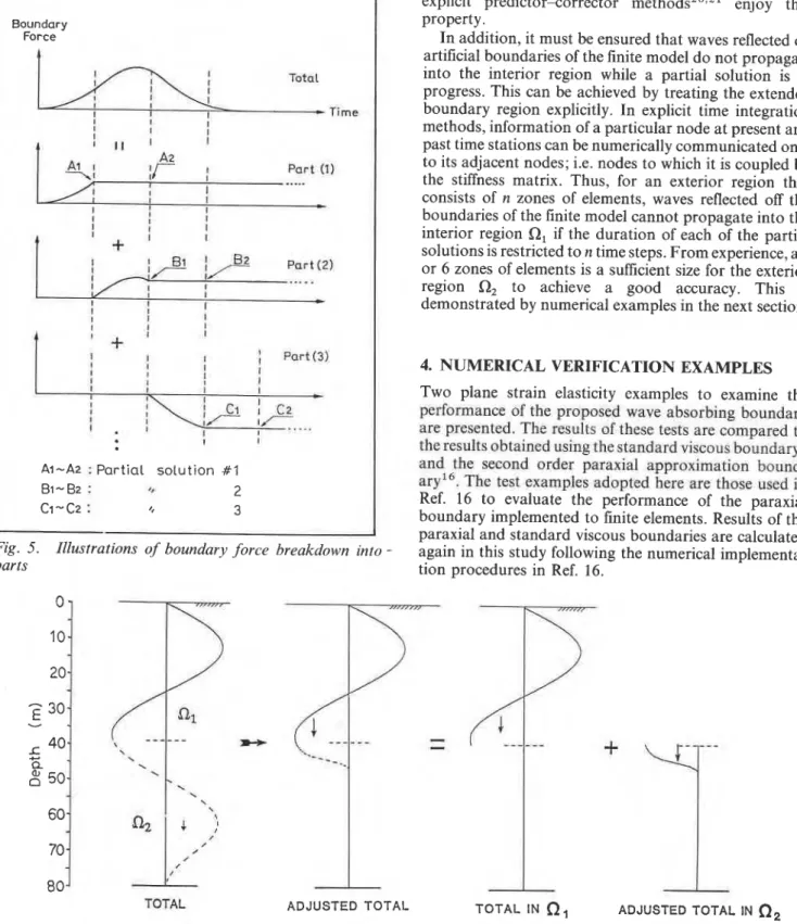
This simple scheme is exactly in line with the concept of breaking the surface load function into parts, as discussed earlier, except that the boundary force F,o,,,,,, is broken into parts as shown in Fig. 5. This breakdown is found to give faster convergence in the partial solution. Convergence here means that degrees of freedom e immediately adjacent to degrees of freedom b achieve zero velocity and zero acceleration in the partial solution. The advantage of the present scheme is that only region Q, needs to be linearly elastic; whereas region Q, can be arbitrarily nonlinear. Regarding the size of the exterior region Q,, it should be large enough so that waves reflected at the artificial boundaries of the finite model do not propagate back into the interior region Q, while a partial solution is in progress.
Reconsidering the shear wave case in a halfspace, discussed at the beginning of this section, a partial solution was started at time 0.70seconds. After convergence at time 0.75 seconds, the response of degrees of freedom e of the total solution was adjusted as explained above. This is illustrated in Fig. 6 for the velocity profile. In Fig. 6, the total response of region Q, was replaced by the adjusted total response, and hence bringing the wave front up from the deep elevations of the model. In order to examine the effect of the adjusted wave field in Q, on the response of region
a,,
the calculations were continued for both the adjusted solution and the original (unadjusted) total solution. In the unadjusted total solution, reflections will start to reach Q, only after time 1.40 seconds. Figure 7 compares the response obtained by these two solutions at time 0.85 seconds. Expectedly, the response of region Ql calculated by the original total solution and that calculated by the adjusted total solution are identical. This implies that no numerical wave shocks have developed. The same procedure is repeated regularly over the duration of the analysis suchSilent boundary for time domain wave motion analyses based on direct energy deletion: M . 0. Al-Hunaidi et al.
that reflections cannot propagate back into the interior region. Calculations of partial solutions are synchronized to operate in parallel fashion with the total solution as shown schematically in Fig. 8. A flowchart of the calculations is also presented in Fig. 9.
3. SIZE OF THE EXTERIOR REGION
The size of the exterior region Q2 has no theoretical restriction except that it will affect the degree of
Boundary Force Total Time I I Part (1) 1 I
;
;
;
I I I I I'r
L"-
1 I B l ' B2 krt:,-,..
I e I I 1 C z I I 1 . I:-
1;-
,... I IAI-A2 : Partial solution #I
81-82 : 2
Cl"C2 : ,, 3
Fig. 5 . Illustrations of boundary force breakdown into -
parts
convergence of the partial solution and, in turn, the accuracy of the proposed wave absorption mechanism. Generally, the larger the exterior region, the better the convergence of the partial solution and, in turn, the more accurate are the results. Convergence depends on the characteristics of the finite elements and time integration algorithm empIoyed. The sudden fixing of the boundary force F,,,,,,, in the partial solution
can
produce highfrequency noises which are familiar in such situations.
Therefore, it is very desirable for the time integration method to have a numerical dissipation property to damp out high frequency noise. Implicit Newmark methods and explicit predictor-corrector method^^^,^^ enjoy this property.
In addition, it must be ensured that waves reflected off artificial boundaries of the finite model do not propagate into the interior region while a partial solution is in progress. This can be achieved by treating the extended boundary region explicitly. In explicit time integration methods, information of a particular node at present and past time stations can be numerically communicated only to its adjacent nodes; i.e. nodes to which it is coupled by the stiffness matrix. Thus, for an exterior region that consists of n zones of elements, waves reflected off the boundaries of the finite model cannot propagate into the interior region Q, if the duration of each of the partial solutions is restricted to n time steps. From experience, a 5 or 6 zones of elements is a sufficient size for the exterior region Cl2 to achieve a good accuracy. This is demonstrated by numerical examples in the next section.
4. NUMERICAL VERIFICATION EXAMPLES
Two plane strain elasticity examples to examine the
performance of the proposed wave absorbing boundary
are presented. The results of these tests are compared to
the results obtained using the standard viscous boundary7 and the second order paraxial approximation bound-
aryi6. The test examples adopted here are those used in Ref. 16 to evaluate the performance of the paraxial boundary implemented to finite elements. Results of the paraxial and standard viscous boundaries are calculated again in this study following the numerical implementa- tion procedures in Ref. 16.
TOTAL ADJUSTED TOTAL TOTAL IN
f l l
ADJUSTED TOTAL INn2
Fig. 6. Wave front brought up from the deep elevation of the model
Silent boundary for time domain wave motion analyses based on direct energy deletion: M. 0. Al-Hunaidi et al.
a1
Unadjusted total solution
,>>
VELOCITY ACCELERATION
Fig. 7. Velocity and acceleration profiles of adjusted and unadjusted total solution at time = 0.85 seconds
-1
-1 :,-I'
---
Fig. 8. Schematic representation of the solution process of the new boundaryThe first test problem is on a 'transient pulse-loading' type which generates high frequency signals. It consists of a vertical pulse load that acts at the surface of a halfspace. This test is chosen to examine the proposed boundary for the reason that it subjects a silent boundary to severe test conditions as the boundary is probably designed to absorb smooth waves16. The second test is designed to examine the capability of a silent boundary to absorb Rayleigh waves. The wave field is generated by subjecting the model to a known Rayleigh wave motion.
Numerical procedures
The continuum is discretized by 4-noded finite elements with bilinear, isoparametric shape functions. Although not necessary for present test problems, the stiffness matrix is divided into a shear (p) part and a lambda
(A)
part (p and A are Lame's constants). The p part is integrated by standard 2 x 2 Gaussian quadrature; whereas the A part is underintegrated by employing standard 1 x 1 Gaussian quadrature. This integration scheme successfully overcomes difficulties experienced when the material approaches incompressible state (i.e. Poisson's ratio approaches 1/2)22. The mass matrix is lumped.
Temporal discretization is performed using an implicit-explicit a l g ~ r i t h m ~ ~ , ~ ~ . This algorithm is a compatible combination of implicit Newmark methods and a corresponding explicit predictor-corrector method.
Fig. 9. Flowchart of the proposed boundary
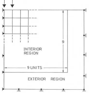
Pulse loading test
The finite element mesh and the corresponding boundary conditions employed for this test problem are shown in Figs 10 and 11, respectively. The wave field is generated by nodal loads as shown in Fig. 11. These loads
. *
Silent boundary for time domain wave motion analyses based on direct energy deletion: M . 0. Al-Hunaidi et al.
TRANSM l TTlNG
BOUNDARY
Fig. 10. Finite element mesh for verticul pulse test
I
INTERIORI
I
REG ION
I
9 UNITS-1
EXTERIOR REGION
Fig. I I . Load con$guration and boundary condition for vertical pulse test
are applied during the first time step and then removed. Material properties of the halfspace are as follows:
c, = 0.5345 units/second, c, = 1.0 units/second, Poisson's ratio=0.3, and density = 1.0. Element size is 1 unit x 1 unit. Exterior region in Fig. 11 designates an extended paraxial element16. It also designates the zone occupied by degrees of freedom e for the proposed boundary, as discussed earlier. For the standard viscous boundary, there is no exterior region. Elements in the interior region are treated implicitly whereas those in the exterior region are treated e x p l i ~ i t l y ~ ~ , ~ ~ . Time step size is 0.9 seconds and the Newmark parameters y and are 0.5 and 0.25, respectively.
Two different sizes for the exterior region of the proposed silent boundary are examined: the first consists of 5 zones of elements and the second consists of 10 zones of elements. As suggested in the previous section, some
Soil Dyi
numerical damping is applied to the model employing the propsed silent boundary but only in the exterior region. The reason for this is to speed up the convergence of partial solutions. Numerical damping can be achieved by assigning the Newmark parameter y a value greater than 0.5. In this example, y in the exterior region of the proposed boundary is set equal to 0.6 with
fl
equal to 0.3025.Response time histories are recorded at two points labelled A and B in Fig. 10 (note: stress is computed at midpoints of elements containing the symbols of these points). The reference solution for the present test is obtained using an extended mesh (28 x 28 implicit elements) in which no reflections propagate into the interior region within the duration of the test. Solutions obtained using silent boundaries are compared to the 'reference solution'. In this way, the evaluation of t!ie performance of silent boundaries is objective because all discretization errors are accounted for in the 'reference solution'.
Vertical displacement, which is the largest component of motion, at points A and B is presented in Figs 12 and 13, respectively. The normal stress, o,,, in x direction, at point B is also presented in Fig. 14. Except for the displacement response at point A, performance of the proposed silent boundary employing a 5 element zones in the exterior region (referred to in figure captions as Energy deletion (5-elements)) is of the same order or superior to the performance of both standard viscous and paraxial boundaries.
Figure 15 presents the results of the proposed silent
Paraxiat - Extended mesh - I I I I I I I I I 0 10 20 30 40 50 Time (sec) Standard viscous--- Extended mesh
-
Energy deletion ---.-
C L ( 5 -element) a Extended mesh-
'
-1.0 1 I 1 I I I I I I 0 10 20 30 40 50 Time (sec) Fig. 12. Calculated time history of vertical displacement at point A caused by impulse loadingSilent boundary for time domain wave motion analyses based on direct energy deletion: M. 0. Al-Hunaidi et al. d
8
-
.-
+- Paraxial L a Extended mesh-
'
-1.0 I 4 I 1 I I I 1 I 0 I0 20 30 40 50 Time (sec) 1.0 I I I 4 I 1 0 U.-
C Standard viscous ---.-
L Extended mesh -9
-1.0 I I I I I I 1 I t 0 10 20 30 4 0 50 Time (sec) 0 U Energy deletion --- ,- + L ( 5 -element) a Extended mesh -=-
-1.0 I 1 1 I 1 I I I 0 10 20 30 40j
50 Time (sec)Fig. 13. Calculated time history of vertical dislacement at point B caused by impulse loading
-a2
!
I I I I I I I I I 0 10 20 30 40 50 Time (sec) 0.2 I I I Standard viscous--- I -0.21
1
0 10 20 30 4 0 50 Time (sec) a2 I I I Energy deletion --- ( 5- element) Extended mesh-
-
5
o
n 0 10 20 30 40 50 Time (sec)Fig. 14. Calculated time history of horizontal normal stress at point B caused by impulse loading
d
s
-
Energy deletion --- -.-
C L (10-element a Extended mesh-
'
-1.0 1 1 I I I I I I 1 0 'I 0 20 30 40 50 Time (sec) 1.0 I ~ n e r ~ ) ; delktion --- at B (10 -element) - - d Extended mesh-
L aJ=
-1.0!
I I I I I I I I 0 10 20 30 40 50 Time (sec) Energy deletion --- 0 -2 - (10-element) II
~xtended mesh --I
1
-0.21
I I I I I I 1 I I 0 10 20 30 40 50 Time (sec)Fig. 15. Prediction of impulse response improved by increasing the size of exterior regions employed in the proposed boundary
boundary employing 10 element zones for the exterior region. Results are almost in exact agreement with the 'reference solution'. Although an exterior region consisting of 10 element zones involves high storage and computational effort, it may be a worthwhile treatment for problems of long time duration and strict accuracy requirements.
Rayleigh wave example
The finite element mesh used in this example is shown in Fig. 16. The mesh is initially at rest. Rayleigh wave field is generated by a displacement controlled harmonic loading applied at the left side of the mesh in Fig. 16. The following known Rayleigh wave field is used (Poisson's ratio is 0.25):
u, = [exp(0.8475kR y)
-0.5773 exp(0.3933kR y)] sin(k,c,t) u,= [-0.8475 exp(0.8475kR y)
+
1.4678 exp(0.3933kR y)] cos(kRcRt) Rayleigh wave number k, = 0.5236, Rayleigh wave velocity c, =0.5312 units/second, shear wave velocity =0.5774 units/second, dilatational wave velocity c,= 1.0 units/second, and density p=1.0. Element size is 1 unit x 1 unit. Elements in both interior and exterior regions are treated explicitly. However, elements over which tractions of the standard viscous boundary act are treated implicitly in order to ensure numerical stability.
.
-
Silent boundary for time domain wave motion analyses based on direct energy deletion: M. 0. Al-Hunaidi et al.
Rayleigh wave input
SILENT
BOUNDARY
Fig. 16. Finite element mesh for Rayleigh wave test
2
1
-1.0 -0 10 20 30 40 50 Time (sec) IDI
Standard viscous-- 1 1 I1
0 10 20 30 40 50 Time (sec)Fig. 17. Calculated time history of vertical displacement at point A caused by Rayleigh wave excitation
.-
0 10 20 30 40 50 Time (sec) 0.5- Standard viscous-- I - d m.-
0 a U.-
C L'
-
0.5 I I I I I 1 I..,
I I 0 10 20 30 4 0 50 Ti me (sec) 0.5-'~neCgy deletion --1-- ' d I l l.-
-0 0 0 U.-
.,- L aJ'
-
0.5 I I I I I I I I I 0 10 20 30 40 50Fig. 18. Calculated time history of vertical displacement at point B caused by Rayleigh wave excitation
.- u
z
0 .,- C 0 N.-
5r Paraxial u I Extended mesh-
4 I I I I I I I I 0 10 20 30 40 50 d m.-
Time step size is 0.9 seconds and Newmark parameters y 73
and /3 are equal to 0.51 and 0.255, respectively, in both
z
C 0interior and exterior regions. Two different sizes of the
;
exterior region of the proposed silent boundary are
.;
considered as in the previous example. o
I Extended mesh
-
Response time histories are recorded at two points -0.2 I I d I I I I I a
labelled A and B in Fig. 16 (note: stress is calculated at 0 10 20 30 Time 40 tsec) 50
midpoints of elements containing these sybmols). The 0.2
I I 1 I I 1 I
'reference solution' is obtained using an extended mesh
that is 28 elements in width. All elements of the extended
$
mesh are treated explicitly.
Vertical displacement response at point A is presented
5
0in Fig. 17; vertical and horizontal displacements as well as
normal stress in y direction a,, atpoint B are presented in .L
-
0 Energy deletion --- Extended mesh
-
Figs 18,19, and 20, respectively. From these figures, it can I ( 5- element 1
be observed that results of the proposed silent boundary -0.2 I I I I I I I 1 I
0 10 20 30 40 50
employing 5 element zones for the exterior region are Time (sec)
superior to the results of both the standard viscous and Fig. 19. Calculated time history of horizontal displace-
paraxial boundaries. Figure 21 demonstrates the ment at point B caused by Rayleigh wave excitation
Soil Dynamics and Earthquake - Engineering, 1990, Vol. 9, No. 2 93 --
L
Silent boundary for time domain wave motion analyses based on direct energy deletion: M . 0. Al-Hunaidi et al.
-0.051 1 4 I I 0 4
b
.20'
i 0'
40 50 Time (sec) 0.05 Extended mesh-
-0.05[
I 4 I I I I 1 4 I 0 10 20 30 40 50 Time (sec)Fig. 20. Calculated time history of vertical normal stress at point B caused by Rayleigh wave excitation
0.2 1 I I I I I d Point (6) In
-
.-
7J B 0 C I 0 N.-
L-
o Extended mesh
-
Energy deletion ---I (10-element) -0.2- I I I I I 1 I I I 0 10 20 30 40 50 Time (sec) "'"dl E E (10-element) Extended mesh
-
g
0 Point (B) -a05I
I I I I I I I I I 0 10 20 30 40 50 Time (sec)Fig. 21. Prediction of Raybigh-wave response improved by increasing the size of exterior region employed in the proposed boundary
improvement in the horizontal displacement and stress
o,, at point B when a 10 element zone is used for the exterior region of the proposed silent boundary.
The results of the standard viscous boundary for the horizontal displacement at point B are particularly disappointing in contrast to the rest of its results. This
shortcoming of the standard viscous boundary under Rayleigh wave excitation was already reported in Ref. 7.
5. CONCLUSIONS
A new wave absorbing boundary has been developed. It is
of the so called 'local type' and hence can be used directly in analyses of semi-discretized systems in the time domain. The wave absorption mechanism is based on direct deletion of wave energy in an extended boundary region. It is demonstrated that this can be achieved through a simple numerical scheme which preserves a wave field continuity that the discretized system can handle without producing numerical wave shocks. High degrees of accuracy can be achieved as it has turned out that the accuracy is a function of the size of the extended boundary region. The larger the boundary region, the better the accuracy.
The silent boundary advocated here is examined using two plane strain elasticity examples: vertical pulse load on half-space and a Rayleigh wave example. Comparisons are made with the well known standard viscous boundary and the second order paraxial approximation boundary. The proposed silent boundary is found to be competitive.
ACKNOWLEDGEMENT
The first author gratefully acknowledges the financial support by the Japanese Ministry of Education, Science and Culture.
REFERENCES
Wolf, J. P. Dynamic Soil-Structure Interaction, Prentice-Hall, 1985
Medina, F. Modelling of soil-structure interaction by finite and infinite elements, UCB/EERC Report, 1980, 80143
Lysmer, J. and Drake, L. A. A finite element method for seismology, Method in Comp. Physics, Academic Press, 1972,11, 181-216
Lysmer, J. and Wass, G. Shear waves in plane infinite structures,
Proc. ASCE, 1972, 98(EM1), 85-105
Werkle, H. Dynamic finite element analysis of three-dimensional soil models with a transmitting element, Earthq. Eng. Struct.
Dyn., 1986, 14(1), 41-60
Kausel, E. and Roesset, J. M. Semianalytic hyperelement for layered strata, Proc. ASCE, 1977, 103(EM4), 569-588 Lysmer, J. and Kuhlemeyer, R. L. Finite dynamic model for infinite media, Proc. ASCE, 1969,95(EM4), 859-877
Joyner, W. B. and Chen, A. T. F. Calculation of nonlinear ground response in earthquakes, Bull. Seism. Soc. Am., 1975, 65(5), 1315-1336
White, W., Valliappan, S. and Lee, I. K. Unified boundary for finite dynamic models, Proc. ASCE, 1977, 103(EM5), 949-964 Akiyoshi, T. Compatible viscous boundary for discrete models,
Proc. ASCE, 1978, 104(EM5), 1252-1265
Akao, Y. and Hakuno, M. Dynamic analysis of wave propagation procedure on the infinite boundary, Proc. JSCE, 1983,336, 21-29
Liao, Z. P. and Wong, H. L. A transmitting boundary for the numerical simulation of elastic wave propagation, Soil Dyn.
Earthq. Eng. 1984, 3(4), 174-193
Smith, W. D. A nonreflecting plane boundary for wave propagation problems, J . Comp. Phys. 1974, 15,492-503 Cundall, P. A,, Kunar, R. R., Carpenter, P. C. and Marti, J. Solution of infinite dynamic problems by finite modelling in the time domain, Proc. 2nd Int. Conf. Appl.. Num. Modelling, Madrid, 1978, 339-351
Clayton, R. and Engquist, B. Absorbing boundary conditions for acoustic and elastic wave equations, Bull. Seism. Soc. Am., 1977, 67(6), 1529-1 540
..
L-
Silent boundary for time domain wave motion analyses based on direct energy deletion: M. 0. Al-Hunaidi et al.
16 Cohen, M. and Jennings, P. C. Silent Boundary Methods for
Transient Analysis, Computational Methods for aansient Analysis, Elsevier, 1983, 301-360
17 Day, S. M. Finite element analysis of seismic scattering problems, Ph.D. Thesis, Univ. California, San Diego, 1977
18 Shiojiri, H. and Nakagawa, T. A method for time-domain analysis of semi-infinite foundation-structure-water systems,
Proc. 5th Int. Conf. Numer. Meth. Geomech., 1985, 2, 883-888
19 Engquist, B. and Kreiss, H . - 0 . Difference and finite element methods for hyperbolic differential equations, Computer
Methods in Applied Mechanics and Engineering, 1979, 17(18), 581-596
20 Hughes, T. J. R. and Liu, W. K. Implicit-explicit finite elements in transient analysis: stability theory, J. Appl. Mech., 1978, 45,
371-374
21 Hughes, T. J. R. and Liu, W. K. Implicit-explicit finite elements in transient analysis: implementation and numerical examples, J.
Appl. Mech., 1978, 45, 375-378.
22 Hughes, T. J. R. Stability of finite elements for nearly incompressible elasticity, J. Appl. Mech., 1977, 44, 181-183
This paper is being distributed in reprint form by the Institute for Research in Construction.
A list of building
practice and research publications available from the Institute may be obtained by writing to Publications Section, Institute for Research in Construction, National Research Council of Canada, Ottawa, Ontario, KIA 0R6.Ce document est distribue sous forme de tirCB-part par 1'Institut de recherche en construction. On peut obtenir une liste des publications de l'lnstitut portant sur les techniques ou les recherches en matiere de Mtiment en ecrivant 21 la Section des publications, Institut de recherche en construction, Conseil national de recherches du Canada, Ottawa (Ontario), KIA 0R6.