Inflation-hedging Portfolios in Different
Regimes
M. Brière
and O. Signori
The unconventional monetary policies implemented in the wake of the subprime crisis and the recent increase in inflation volatility have revived the debate on medium to long-term resurgence of inflation. This paper presents the optimal strategic asset allocation for investors seeking to hedge inflation risk. Using a vector-autoregressive model, we investigate the optimal choice for an investor with a fixed target real return at different horizons, with shortfall probability constraint. We show that the strategic allocation differs sharply across regimes. In a volatile macroeconomic environment, inflation-linked bonds, equities, commodities and real estate play an essential role. In a stable environment (“Great Moderation”), nominal bonds play the most significant role, with equities and commodities. An ambitious investor in terms of required real return should have a larger weighting in risky assets, especially commodities.
JEL Classifications: E31, G11, G12, G23
Keywords: inflation hedge, pension finance, shortfall risk, portfolio optimisation
CEB Working Paper N° 09/047
2009
Inflation-hedging Portfolios in Different Regimes
M. Brière
1,2and O. Signori
2,*Abstract
The unconventional monetary policies implemented in the wake of the subprime crisis and the recent increase in inflation volatility have revived the debate on medium to long-term resurgence of inflation. This paper presents the optimal strategic asset allocation for investors seeking to hedge inflation risk. Using a vector-autoregressive model, we investigate the optimal choice for an investor with a fixed target real return at different horizons, with shortfall probability constraint. We show that the strategic allocation differs sharply across regimes. In a volatile macroeconomic environment, inflation-linked bonds, equities, commodities and real estate play an essential role. In a stable environment (“Great Moderation”), nominal bonds play the most significant role, with equities and commodities. An ambitious investor in terms of required real return should have a larger weighting in risky assets, especially commodities.
Keywords: inflation hedge, pension finance, shortfall risk, portfolio optimisation JEL codes: E31, G11, G12, G23
1
Université Libre de Bruxelles
Solvay Brussels School of Economics and Management Centre Emile Bernheim
Av. F.D. Roosevelt, 50, CP 145/1 1050 Brussels, Belgium.
2
Crédit Agricole Asset Management, 90 bd Pasteur, 75015 Paris, France
* Comments can be sent to [email protected], or [email protected].
The authors would like to thank A. Attié, U. Bindseil, U. Das, B. Drut, J. Coche, C. Mulder, K. Nyholm, M. Papaioannou, S. Roache, E. Schaumburg, A. Szafarz and the participants to the BIS/ECB/World Bank Public Investors Conference for helpful comments and suggestions.
1. Introduction
Having weathered the worst crisis in terms of length and amplitude since the Second World War, investors could have to cope with one of the potential outcomes of the subprime meltdown: the threat of a surge in the cost of living. The accumulation of multiple factors raises the question as to whether a globally low and stable inflation environment can continue to exist (Barnett and Chauvet (2008), Cochrane (2009), Walsh (2009)), thereby raising the key concern of inflation hedging for many investors. To support weak economies almost all developed countries applied unconventional monetary policies with significant stimulus packages and injections of liquidity into money markets. The exceptional rise in government deficits and huge debt levels are a looming problem for the US and many European countries, while the recent oil price spike, dollar weakness and macroeconomic volatility are adding further pressures to the ongoing debate. These renewed concerns about inflation naturally raise the question of re-considering how to build the ideal portfolio that will shield investors effectively from inflation risk and, where possible, generate excess returns. This applies both to long-term institutional investors (particularly pension funds, which operate under inflation-linked liability constraints) and to individual investors, for whom real-term capital preservation is a minimal objective.
Consider an investor having a target real return and facing inflation risk. Her portfolio is made of Treasury bills, government nominal and inflation-linked (IL) bonds, stocks, real estate and commodities. Three questions are to be solved. (1) What is the inflation hedging potential of each asset class? (2) What is the optimal allocation for a given target return and investment horizon? (3) What is the impact of changing economic environment on this allocation? To address those questions, we consider a two-regime approach, macroeconomic
volatility is either high, as it was during the 1970s and 1980s, or low, as in the 1990s and 2000s marked by the “Great Moderation”.
We use a vector-autoregressive (VAR) specification to model the inter-temporal dependency across variables, and then simulate long-term holding portfolio returns up to 30 years. Recent research has pointed to instability and regime shifts in the stochastic process generating asset returns. Guidolin and Timmerman (2005), and Goetzmann and Valaitis (2006) stress that a full-sample VAR model can be mis-specified as correlation vary over time. Asset returns exhibit multiple regimes (Garcia and Perron (1996), Ang and Bekaert (2002), Connolly et al. (2005)).The changing economic conditions and the strong decrease in macroeconomic volatility (the “Great Moderation”, Blanchard and Simon (2001), Bernanke (2004), Summers (2005)) has been stressed as one of the main factors affecting the level of stocks and bond prices (Lettau et al. (2008), Kizys and Spencer (2008)), also partially explaining the changing correlation between stocks and bonds returns (Baele et al. (2009)). Using the Goetzmann et al. (2005) breakpoint test for structural change in correlation, we split the sampling period into 2 sub-periods exhibiting the most stable correlations. The simulated returns based on our two estimated VAR models are thus used, on the one hand, to measure the inflation hedging properties of each asset class in each regime, and on the other hand to carry out a portfolio optimisation in a mean-shortfall probability framework. We determine the allocation that maximises above-target returns (inflation + x%) with the constraint that the probability of a shortfall remains lower than a threshold set by the investor.
We show that the optimal asset allocation strongly differs across regimes. In the periods of highly volatile economic environment, an investor having a pure inflation target should be mainly invested in cash when his investment horizon is short, and increase his
allocation to IL bonds, equities, commodities and real estate when his horizon increases. In contrast, in a more stable economic environment, cash plays an essential role in hedging a portfolio against inflation in the short run, but in the longer run it should be replaced by nominal bonds, and to a lesser extent by commodities and equities. With a more ambitious real return target (from 1% to 4%), a larger weight should be dedicated to risky assets (mainly equities and commodities). These results confirm the value of alternative asset classes in shielding the portfolio against inflation, especially for ambitious investors with long investment horizons.
Our paper tries to complement the existing literature in 3 directions: inflation hedging properties of assets, strategic asset allocation, and alternative asset classes. The question of hedging assets against inflation has been widely studied (see Attié and Roache (2009) for a detailed literature review). Most studies have focused on measuring the relationship between historical asset returns and inflation, either by measuring the correlation between these variables or by adopting a factor approach such as the one used by Fama and Schwert (1977). These approaches present a number of difficulties, especially with regard to the lack of historical data available to study long-horizon returns, the problem of non-serially independent data, non-stationary variables, and instability over time of the assets’ relationships to inflation.
The literature on strategic asset allocation has shed new light on this question. Continuing the pioneering work of Brennan et al. (1997), Campbell and Viceira (2002), many researchers have sought to show that long-term allocation is very different from short-term allocation when returns are partially predictable (Barberis (2000), Brennan and Xia (2002), Wachter (2002), Campbell et al. (2003, 2004), Guidolin and Timmermann (2005), Fugazza et
al. (2007)). The approach developed in an assets-only framework was extended to Assets and Liabilities Management (ALM) using traditional classes (van Binsbergen and Brandt (2007)) but also alternative assets (Goetzmann and Valaitis (2006), Hoevenaars et al. (2008), Amenc et al. (2009)). One common characteristic of these studies is their focus on the situation of investors with liabilities, such as pension funds, which are subject to the risk of both fluctuating inflation and real interest rates. In this article, we adopt a different point of view. Not all investors who seek to hedge against inflation necessarily have such liabilities. They may only wish to hedge their assets against the risk of real-term depreciation, and thus have a purely nominal objective that consists of the inflation rate plus a real expected return target, which is assumed to be fixed.
Thus far, most of the research into inflation hedging for diversified portfolios has been done within a mean-variance framework. The studies of inflation hedging properties in an ALM framework with a liability constraint generally focus on a “surplus optimisation” (Leibowitz (1987), Sharpe and Tint (1990), Hoevenaars et al. (2008)). In our context, however, this risk measure is not the one that corresponds best to investors’ objectives. Our portfolio’s excess returns above target may be only slightly volatile but still significantly lower than the objective, presenting a major risk to the investor. The notion of “safety-first” (Roy (1952)) is therefore more appropriate. We focus on the shortfall probability, i.e. the likelihood of not achieving the target return at maturity. In an ALM framework, Amenc et al. (2009) measure shortfall probability of ad hoc portfolios. We expand that work and determine optimal portfolio allocations in a mean/shortfall probability framework.
The properties of alternative asset classes have been studied in a strategic asset allocation context (Agarwal and Naik (2004), Fugazza et al. (2007), Brière et al. (2010)). In
an ALM context, Hoevenaars et al. (2008) and Amenc et al. (2009) also find significant appeal in these asset classes, which are interesting sources of diversification and inflation hedging in a portfolio. To the best of our knowledge, however, these asset classes have not yet been studied in an asset only context with an inflation target. Our research tries to fill the gap.
Our paper is organised as follows. Section 2 presents our data and methodology. Section 3 presents our results: correlation structure of our assets with inflation at different horizons, optimal composition of inflation hedging portfolios. Section 4 concludes.
2. Data and methodology
2.1 Data
We consider the case of a US investor able to invest in six liquid and publicly traded asset classes: cash, stocks, nominal bonds, IL bonds, real estate and commodities. (1) Cash is the 3-month T-bill rate. (2) Stocks are represented by the Morgan Stanley Capital International (MSCI) US Equity index. (3) Nominal bonds are the Morgan Stanley 7-10 year index. (4) IL bonds are represented by the Barclays Global Inflation index from 19971. Before that date, to recover price and total return history before IL Bonds were first issued in the US, we reconstruct a time series of real rates according to the methodology of Kothari and Shanken (2004). Real rates are thus approximated by 10-year nominal bonds rates minus an inflation expectation based on a 5-year historical average of a seasonally adjusted consumer price index (CPI) (Amenc et al. (2009)). The inflation risk premium is assumed equal to zero,
1
a realistic hypothesis considering the recent history of US TIPS (Berardi (2004), D’Amico et al. (2008), Brière and Signori (2009)). (5) Real estate investments are proxied by the FTSE NAREIT Composite Index representing listed real estate in the US (publicly traded property companies of NYSE, Nasdaq, AMEX and Toronto Stock Exchange). (6) Commodities are represented by the Goldman Sachs Commodity Index (GSCI). We also add a set of exogenous variables: inflation (measured by the CPI), dividend yield obtained from the Shiller database (Campbell and Shiller (1988)) and the term spread measured as the difference between 10-year Treasury Constant Maturity Rate and 3-month Treasury bill rate provided by the US Federal Reserve Economic Database. We consider monthly returns on the time period January 1973 – June 2009.
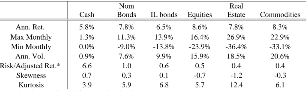
Table 1 in Appendix 1 presents the descriptive statistics of monthly returns. The hierarchy of returns is the following: cash has the smallest return on the total period, followed by IL bonds, nominal bonds, real estate, equities and commodities. Adjusted for risk, the results show a slightly different picture: cash appears particularly attractive compared to other asset classes, nominal bonds are much more appealing than real estate (risk-adjusted return of 1 vs 0.4), and equities are more attractive than commodities (0.5 vs 0.4). Extreme risks are also different: negative skewness and strong kurtosis are really pronounced for real estate and to a lesser extent for equities and commodities.
2.2 Econometric model of asset returns dynamics
VAR models are widely used in financial economics to model the intertemporal behaviour of asset returns. Campbell and Viceira (2002) provide a complete overview of the
applications of VAR specification to solve intertemporal portfolio decision problems. The VAR structure can also be used to simulate returns in the presence of macroeconomic factors. Following Barberis (2000), Campbell et al. (2003), Campbell and Viceira (2005), Fugazza et al. (2007)) among others, we adopt a VAR(1) representation of the returns but expand it to alternative asset classes, as did Hoevenaars et al. (2008)2. Empirical literature has relied on a predetermined choice of predictive variables. Kandel and Stambaugh (1996), Balduzzi and Lynch (1999), Barberis (2000) use the dividend yield; Lynch (2001) uses the dividend yield and term spread; Brennan, Schwartz, and Lagnado (1997) use the dividend yield, bond yield, and Treasury bill yield; and Hoevenaars et al. (2008) use the dividend yield, term spread, credit spread and Treasury bill yield. We select the most significant variables in our case: dividend yield and term spread. As we are modelling nominal logarithmic returns, we also enter inflation explicitly as a state variable, which enables us to measure the link between inflation and asset class returns3.
The compacted form of the VAR(1) can be written as:
t t
t z u
z =φ0 +φ1 −1 + (1)
where φ0is the vector of intercepts; φ is the coefficient matrix; 1 z is a column vector whose t
elements are the log returns on the six asset classes and the values of the three state variables ;
t
u is the vector of a zero mean innovations process.
2
The differences with the model lie in the fact that we include IL bonds but not corporate bonds and hedge funds in our investment set. As our investor is an asset-only investor, there are no liabilities in our model.
3
As in the models of Brennan et al. (1997), Campbell and Viceira (2002), Campbell et al. (2003), we do not adjust VAR estimates for possible small sample biases related to near non-stationarity of some series (Campbell and Yogo (2006)).
Finally, to overcome the problem of correlated innovations of the VAR(1) model and to obtain structural innovations characterised by a iid process we follow the procedure described in Amisano and Giannini (1997). The structural innovationsεt, may be written as
t
t B
Au = ε where the parameters of A and B matrices are identified imposing a set of restrictions. The structure of εt is used to perform Monte Carlo simulations on the estimated
VAR for the portfolio analysis.
Meaningful forecasts from a VAR model rely on the assumption that the underlying sample correlation structure is constant. However, regime shifts in the relationship between financial and economic variables have already been widely discussed in the literature. Guidolin and Timmermann (2005), Goetzmann and Valaitis (2006) find evidence of multiple regimes in the dynamics of asset returns. This suggests that a full-sample VAR model might be potentially mis-specified, as the correlation structure may not be constant. The changing macroeconomic volatility has been identified as one of the main causes of the changing correlation structure between assets (Li (2002), Ilmanen (2003), Baele et al. (2009)), Using the Goetzmann et al. (2005) test4 for structural change in correlations between asset returns and state variables, we determine the breakpoint that best separates the sample data, ensuring the most stable correlation structure within each sub-period5. The first period (January 1973-December 1990) corresponds to a volatile economic environment (large oil shocks, huge government deficits, large swings in GDP growth), the second (January 1991- June 2009) to a much more stable one.
4
Null hypothesis of stationary bivariate historical correlations between assets. 5
Tables 2 to 5 in Appendix 1 present the results of our VAR model in the two identified sub-periods. Looking at the significance of the coefficients of the lagged state variables, inflation is mainly helpful in predicting nominal bond returns. Dividend yield has better explanatory power for equity returns in the second period than in the first. The high positive correlation coefficient of the residuals between nominal bonds and IL bonds (84% and 76% in the two sub-sample periods) confirms the strong interdependency between the contemporaneous returns of the two asset classes dominated by the common component of real rates. Real estate and equities have the second largest positive correlation (61% and 55% respectively). Other results are in line with the common findings of positive contemporaneous correlation between inflation and commodities, and the intuition that inflation and monetary policy shocks have a negative impact on bonds returns through the inflation expectations component.
2.3 Simulations
We use the iid structural innovation process of the two VAR models estimated on the two sub-samples to perform a Monte Carlo analysis based on the fitted model. We draw iid random variables from a multivariate normal distribution for the structural innovations and we obtain simulated returns for 5000 simulated paths of length T (T varying from 1 month to 30 years). The simulated returns are thus used, on the one hand, to measure the inflation hedging properties of each asset class in each regime, and on the other hand in a portfolio construction context to generate expected returns and covariance matrices at different horizons (2, 5, 10, 30 years).
2.4 Portfolio choice
The bulk of the research into inflation hedging for a diversified portfolio has used a mean-variance framework. And research into inflation hedging properties in an ALM framework with a liability constraint is usually based on surplus optimisation, in which the surplus is maximised under the constraint that its volatility be lower than a target value (Leibowitz (1987), Sharpe and Tint (1990), Hoevenaars et al. (2008)). But for our purposes, this risk measure is not the one best suited to investors’ objectives. Since the portfolio’s excess returns above target may be only slightly volatile but still significantly lower than the objective, the investor faces a serious risk. In this case, the notion of safety-first (Roy (1952)) is more appropriate. Roy argues that investors think in terms of a minimum acceptable outcome, which he calls the “disaster level”. The safety-first strategy is to choose the investment with the smallest probability of falling below that disaster level. A less risk averse investor may be willing to achieve a higher return, but with a greater probability of going below the threshold. Roy defined the shortfall constraint such that the probability of the portfolio’s value falling below a specified disaster level is limited to a specified disaster probability. Portfolio optimisations with a shortfall probability risk measure have been conducted before (Leibowitz and Henriksson (1989), Leibowitz and Kogelman (1991), Lucas and Klaassen (1998), Billio (2007), Smith and Gould (2007)), but as far as we know not in the context of an inflation hedging portfolio.
We determine optimal allocations that maximise above-target returns (the target being inflation + x%) with the constraint that the probability of a shortfall remains lower than a threshold set by the investor.
⎥ ⎦ ⎤ ⎢ ⎣ ⎡ + −
∑
= ) ( 1 R R w E Max T n i iT i w π (1) α π + < <∑
= ) ( 1 R R w P T n i iT i (2) 1 1 =∑
= n i i w (3) 0 ≥ i w (4)Where )RT =(R1T,R2T,...,RnT is the annualised return of the n assets in portfolio over the investment horizon T, )w=(w1,w2,...,wn the fraction of capital invested in the asset i,π the T
annual inflation rate during that horizon T, R the target real return in excess of inflation, and α the target shortfall probability. E is the expectation operator with respect to the probability distribution P of the asset returns.
We work in a mean-shortfall probability world and derive the corresponding efficient frontier (Harlow (1991)). For a portfolio with normally distributed returns N(μ,σ), the probability of portfolio shortfall is written:
p w R R Re dx x T T T
∫
−∞+ − − = + < π σ μ σ π π 2 2 2 ) ( 2 1 ) ' (For each investment horizon T (T = 1 year, 3 years, 5 years, 10 years, 20 years, 30 years), we draw all the efficient portfolios in the mean-shortfall probability universe for the two identified regimes.
3. Results
3.1 Inflation hedging properties of individual assets
Figures 1 and 2 in Appendix 1 display correlation coefficients between asset returns and inflation based on our VAR model, depending on the investment horizon, from 1 month to 30 years. We consider two sample periods: from January 1973 to December 1990 and from January 1991 to June 2009. The inflation hedging properties of the different assets vary strongly depending on the investment horizon. Most of the assets (the only exception being commodities and nominal bonds in the first period) display an upward-sloping correlation curve, meaning that inflation hedging properties improve as the investment horizon widens.
In the first sample period (1973-1990), marked by a volatile macroeconomic environment, cash and commodities have a positive correlation with inflation on short-term horizons, whereas nominal bonds, equities, and real estate are negatively correlated. The correlation of IL bonds with inflation lies in the middle and is close to zero. In the longer run (30 years), cash shows the best correlation with inflation (around 0.6), followed by IL bonds and real estate (all showing a positive correlation), then equities, commodities, and finally nominal bonds (the latter with negative correlation).
The very strong negative correlation of nominal bonds, with inflation both in the short run and in the long run, is intuitive since changes in expected inflation and bond risk premiums are traditionally the main source of variation in nominal yields (Campbell and Ammer (1993)). IL bonds and inflation are positively correlated for an obvious reason: the impact of a strongly rising inflation rate has a direct positive impact on performances through
the coupon indexation mechanism. Negative correlation between equities and inflation has been documented by many authors, with three different interpretations. The first is that inflation hurts the real economy, so the dividend growth rate should fall, leading to a fall in equity prices (an alternative explanation is that poor economic conditions lead the central bank to lower interest rates, which has a positive influence on inflation (Geske and Roll (1983)). The second interpretation argues that high expected inflation has tended to coincide with periods of higher uncertainty about real economic growth, raising the equity risk premium (Brandt and Wang (2003), Bekaert and Engstrom (2009)). The final explanation is that stock market investors are subject to inflation illusion and fail to adjust the dividend growth rate to the inflation rate, even though they adjust correctly the nominal bond rate (Modigliani and Cohn (1979), Ritter and Warr (2002), Campbell and Vuolteenaho (2004)). Commodities exhibit more contrasted behaviour, i.e. the correlation with inflation is positive in the short run but negative in the long run. This result is consistent with the fact that commodities have a tendency to overreact to money surprises (and therefore inflation) in the short run (Browne and Cronin (2007)), whereas the long-term link with inflation has been weak since the 1980s, when the commodity-consumer price connection seems to have broken down. This reflects the diminished role of traditional commodities in US production and the sterilisation of some inflation signals by offsetting monetary policy actions (Blomberg and Harris (1995), Hooker (2002)).
The correlation picture is very different if we now consider the second sample period (1991-2009), marked by a stable macroeconomic environment. The hierarchy of the different assets in terms of inflation hedging properties is very different, both in the long run and in the short run. In the short run, commodities have the strongest correlation with inflation, followed by cash, real estate, nominal bonds, IL bonds and equities. In the long run, the best inflation hedger is now cash, followed by equities, real estate, nominal bonds, IL bonds and
commodities. The main differences with the first period are that nominal bonds and equities now have a positive correlation with inflation in the long run, and better inflation hedging properties than IL bonds. The moderation in economic risk, especially inflation volatility, has reduced correlations in absolute terms. IL bond returns have a much smaller positive correlation with inflation, whereas nominal bonds lose their negative correlation and become moderately positively correlated. This changing behaviour is strongly linked to the much stronger credibility and transparency of central banks in fighting inflation during the last two decades, leading to more stable and lower interest rates, only slightly impacted by inflation changes (Kim and Wright (2005), Eijffinger et al. (2006)).
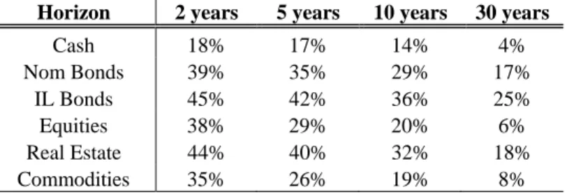
Another way to look at the inflation hedging properties of individual assets is to measure the probability of having below-inflation returns at the investment horizon (shortfall probabilities). Tables 6 and 7 in Appendix 1 display the shortfall probabilities of the different asset classes for horizons of 2, 5, 10 and 30 years. A first observation is that shortfall probabilities decrease strongly with the investment horizon. This is true for all asset classes, but particularly for the most risky ones. Commodities, for example, have a probability of not achieving the inflation target of more than 35% at a 2-year horizon. At 30 years, this falls below 8% for both periods. An asset can be strongly correlated with inflation but also have a significant shortfall probability if its return is always lower than inflation. Looking at shortfall probabilities, the best inflation hedger in the short run appears to be cash on both inflation regimes. In the long run, the best hedgers are cash, equities and commodities in the volatile regime (IL bonds are well correlated with inflation during that period but with a strong shortfall probability, 25% for a 30-year horizon), and nominal bonds and commodities in the stable regime.
3.2 Inflation hedging portfolios
We now turn to the construction of inflation hedging portfolios. We examine the case of an investor wishing to hedge inflation on his investment horizon. This investor has a target real return ranging from 0% to 4%. For each of the investor targets, we show the optimal portfolio composition depending on the inflation regime.
How to attain pure inflation target
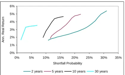
We first consider the case of an investor simply wishing to hedge inflation, i.e. having a target real return of 0%. In a mean-variance analysis, the Markowitz frontier describes the tradeoff between the expected value and standard deviation of the portfolio return. Likewise, Figures 3 and 4 show the tradeoff between shortfall probability and expected above-target returns on each of the two sample periods. Each curve represents a different investment horizon (2, 5, 10 and 30 years). Table 8 and Table 13 in Appendix 2 show the optimal portfolio composition and the descriptive statistics of minimum shortfall probability portfolios for each horizon.
Figure 3 : Efficient frontiers, expected return above inflation and shortfall probability tradeoff, January 1973-December 1990.
Figure 4 : Efficient frontiers, expected return above inflation and shortfall probability tradeoff, January 1991-June 2009.
The first observation, common to both periods, is that efficient frontiers are all upwardly sloped. This is consistent with intuition: the higher the required return, the greater the shortfall probability in the portfolio. The minimum shortfall probability (corresponding to Roy’s (1952) “safety-first” portfolio) generally decreases with the investment horizon, the
0% 1% 2% 3% 4% 5% 6% 0% 5% 10% 15% 20% 25% 30% 35% Shortfall Probability A n n. R e al R e tu rn
2 years 5 years 10 years 30 years
0% 1% 2% 3% 4% 5% 6% 0% 5% 10% 15% 20% 25% 30% 35% Shortfall Probability A n n . R eal R e tur n
only exception being for the 2-year horizon on the first period, where the minimum shortfall probability is lower than for the 5-year horizon.
In the first period, characterised by high macroeconomic volatility, the optimal portfolio composition of a “safety-first” investor with a 2-year horizon is 88% cash, 6% IL bonds, 1% equities and 5% commodities. This very conservative portfolio has a 1.6% annualised return over inflation, 1.9% volatility of real returns and 11% shortfall probability. Diversifying the portfolio makes it possible to sharply diminish the achievable shortfall probability compared to individual assets: whereas the minimum shortfall probability over all assets in that period is 18% (for cash), it is 7% lower with a diversified portfolio. When the horizon is increased, the weight assigned to cash decreases and the weights of riskier assets (IL bonds, equities, real estate, commodities) rise. For a 30Y horizon, the optimal portfolio composition is 64% cash, 17% IL bonds, 8% equities, 5% real estate and 6% commodities. This portfolio generates an annualised excess return of 2.2% over inflation with stronger volatility (5.4%) but with a very low probability (1.4%) of falling above the inflation target at the investment horizon. Again, portfolio diversification makes it possible to decrease strongly the shortfall probability at the investment horizon.
In the second period, characterised by much low macroeconomic volatility, the optimal portfolio composition is quite different. With a 2Y horizon, the optimal composition for a “safety-first” investor is still very conservative: 81% cash, but the rest of the portfolio consists mainly of nominal bonds (17%), real estate (1%) and commodities (2%). Compared to the first period, nominal bonds now replace IL bonds and equities. This result is consistent with our previous findings on individual assets: the inflation hedging properties of nominal bonds increase strongly in the second period, with inflation correlation becoming even greater
than for IL bonds and shortfall probabilities becoming much smaller. Increasing the investment horizon, the share of the portfolio dedicated to cash decreases, progressively replaced by nominal bonds, whereas the weights of commodities and equities increase slightly. With a 30 year horizon, the optimal portfolio of a “safety-first” investor is composed of 73% nominal bonds, 10% equities and 17% commodities. This portfolio has slightly higher annualised real return than in the first period (3.2% vs. 2.2%), with a smaller shortfall probability (0.02% vs. 1.4%). Contrary to the first period, IL bonds no longer appear in the optimal composition of safety-first portfolios.
To sum up, when macroeconomic volatility is high, a “safety-first” investor having a pure inflation target should be mainly invested in cash when his investment horizon is short, and should increase his allocation to IL bonds, equities, commodities and real estate when his horizon increases. When economic volatility is much lower, the optimal investment set changes radically. Mainly invested in cash when the investment horizon is short, an investor should increase his holdings of nominal bonds, commodities and equities when his investment horizon increases.
Raising the level of required real return
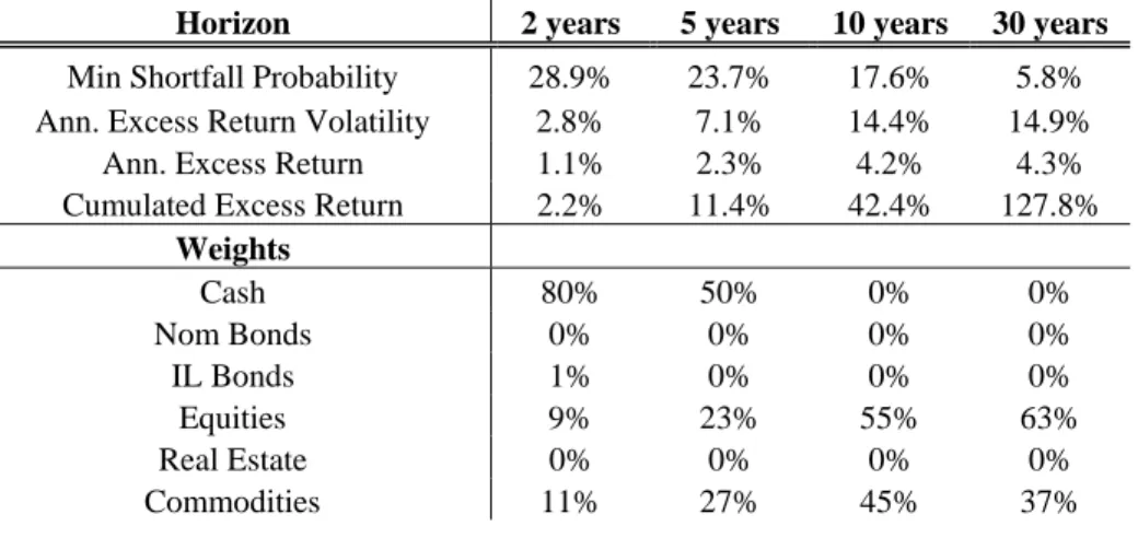
We now consider the consequences for an investor of having a more ambitious target real return, ranging from 1% to 4%. Tables 9 to 12 and 14 to 17 in Appendix 2 present the optimal portfolio composition as well as the descriptive statistics of the minimum shortfall probability portfolios, for the first and second sample periods.
Consistent with intuition, when the required real return is increased, the shortfall probability increases strongly in both sub-periods. In the first period, for a 2Y horizon investor, the minimum shortfall probability is 10.8% for a target real return of 0%. It is 28.9%, 36.7%, 40.9% and 44.0% for a 1%, 2%, 3% and 4% real target return respectively. The results are similar for the second period: shortfall probabilities rise from 4.7% to 44.9% for a 0% to 4% real return target.
Another intuitive result is that the more the investor increases his required real return, the more the optimal portfolio composition is biased towards risky assets. Considering the first period, for a 30-year horizon, the optimal weight of cash decreases from 64% (with a real return target of 0%) to 0% (1% to 4% target). The IL bond weight also decreases, from 17% to 0%. The explanation is intuitive: these assets provide a good inflation hedge but are not sufficient to achieve high real returns. On the contrary, the weights of risky assets (equities, and especially commodities) increase. A long-term portfolio seeking to achieve inflation +1% should comprise 63% equities and 37% commodities. With a 4% target, the investor should hold 32% equities and 68% commodities. Of course, if the investment horizon is shorter, a more substantial part of the portfolio should be dedicated to cash.
In the second sample period, the results are comparable. Increasing the real return target leads to a decrease in the cash investment and an increase in the more risky assets. The difference lies in the “risky” assets retained by the optimisation. A substantial portion of nominal bonds should now be added to the optimal mix of equities and commodities than in the first period. For a 30-year investors with 1% real return target, the optimal portfolio composition is 69% nominal bonds, 10% equities and 21% commodities. It is 60% bonds, 9% equities and 31% commodities for a 2% target, and 100% commodities for a 3% and 4%
target. As in the first period, commodities are the most rewarding asset class. This explains why, with a very ambitious real return target, the portfolio should be fully invested in commodities.
To sum up, a more ambitious real return target leads to a greater shortfall probability and a different optimal portfolio composition, with a larger weight in risky assets. In an unstable and volatile economic regime, an ambitious investor should abandon IL bonds and real estate and concentrate on equities and commodities. In a more stable economic environment, he should reduce his portfolio weight in nominal bonds and equities and invest a higher share in commodities.
4. Conclusion
A key challenge for many institutional investors is the preservation of capital in real terms, while for individual investors it is building a portfolio that keeps up with the cost of living. In this paper we address the investment problem of an investor seeking to hedge inflation risk and achieve a fixed target real rate of return. The key question is thus to determine the optimal asset allocation that will preserve the investor’s capital from inflation with an acceptable probability of shortfall.
Following Campbell et al. (2003), Campbell et Viceira (2005), we used a vector-autoregressive (VAR) specification to model the joint dynamics of asset classes and state variables, and then simulated long-term holding portfolio returns for a range of different assets and inflation. The strong change in macroeconomic volatility has been identified as one
of the main causes of the changing correlation structure between assets (Li (2002), Ilmanen (2003), Baele et al. (2009). Using the Goetzmann et al. (2006) test for structural change in correlation, we determined the breakpoint that best separates the sample data, ensuring the most stable correlation structure within each sub-period. We estimated a VAR model on each period and performed a simulation-based analysis. This made it possible to measure the inflation hedging properties of each asset class in each regime and to determine the allocation that maximises above-target returns (inflation + x%) with the constraint that the shortfall probability remains lower than a threshold set by the investor.
Our results confirm that the presence of macroeconomic volatility regimes changes radically the investor’s optimal allocation. In a volatile regime, a “safety-first” investor having a pure inflation target should be mainly invested in cash when his investment horizon is short, and should increase his allocation to IL bonds, equities, commodities and real estate when horizon increases. In a more stable economic environment, the optimal investment set changes radically. Mainly invested in cash when investment horizon is short, an investor should increase his investment in nominal bonds, but also, to a lesser extent, to commodities and equities when his horizon increases. Our results confirm the value of alternative asset classes in protecting the portfolio against inflation.
Having a more ambitious real return target (from 1% to 4%) leads automatically to a greater shortfall probability, but also to a different optimal portfolio composition. A larger weight should be dedicated to risky assets, which make it possible to achieve higher returns (with a greater shortfall probability). In the first period, an ambitious investor should gradually abandon IL bonds and real estate and concentrate on equities and particularly
commodities. In the second period, he should reduce his portfolio weight in nominal bonds and equities and invest a higher share in commodities.
Our work could be extended in several ways. Different methodologies have been developed that move away from the standard mean-variance approach, by changing the risk measure of the portfolio. One branch of the literature considers portfolio selection with Value at Risk (Agarwal and Naik (2004), Martellini and Ziemann (2007)), or conditional VaR (Rockafellar and Uryasev (2000)); the other branch with shortfall probability (Leibowitz and Henriksson (1989), Leibowitz and Kogelman (1991), Lucas and Klaassen (1998), Billio and Casarin (2007), Smith and Gould (2007)). A useful development of our work would be to reconcile the two approaches and examine shortfall probabilities in the context of non-normal returns. We have considered only a static allocation on the whole investment horizon. A very interesting development would be to compare these results with a dynamic asset allocation, rebalancing the portfolio depending on active views on the different asset classes. Finally, we examined a fairly simple objective function. In the real world, many investors (especially pension funds) do not have a single well-defined goal but rather have to cope with multiple and sometimes contradictory objectives, with long-term return shortfall probability constraints and short term performance objectives. An interesting development of this work would be to take these different constraints into account.
References
Agarwal, V., Naik, N., 2004. Risks and Portfolio Decisions Involving Hedge Funds. Review of Financial Studies, 17(1), 63–8.
Amenc, N., Martellini, L., Ziemann, V., 2009. Alternative Investments for Institutional Investors, Risk Budgeting Techniques in Asset Management and Asset-Liability Management. The Journal of Portfolio Management, 35(4), Summer, 94-110.
Amisano, G., Giannini, C., 1997. Topics in structural VAR econometrics, Second edition, Berlin and New York: Springer.
Ang, A., Bekaert, G., 2002. International Asset Allocation with Regime Shifts. Review of Financial Studies, 15, 1137-1187.
Attié, A.P., Roache, S.K., 2009. Inflation Hedging for Long-Term Investors. IMF Working Paper, No. 09-90, April.
Baele, L., Bekaert ,G., Inghelbrecht, K., 2009. The Determinants of Stock and Bond Return Comovements. NBER Working Paper, No. 15260, August.
Balduzzi, P., Lynch, A.W., 1999. Transaction Costs and Predictability: Some Utility Cost Calculations. Journal of Financial Economics, 52, 47-78.
Barberis, N., 2000. Investing for the Long Run when Returns are Predictable. The Journal of Finance, 40(1), February, 225-264.
Barnett, W., Chauvet, M., 2008. The End of Great Moderation?. University of Munich, Working Paper.
Bekaert, G., Engstrom, E., 2009. Inflation and the Stock Market: Understanding the Fed Model. NBER Working Paper, No. 15024, June.
Berardi, A., 2005. Real Rates, Excepted Inflation and Inflation Risk Premia Implicit in Nominal Bond Yields. Università di Verona Working Paper, October.
Bernanke, B., 2004. The Great Moderation. Remarks at the meetings of the Eastern Economic Association, Washington, DC, February 20.
Billio, M., Casarin, R., 2007. Stochastic Optimization for Allocation Problems with Shortfall Constraints, Applied Stochastic Models in Business and Industry, 23(3), May, 247-271.
van Binsbergen, J.H., Brandt, M.W., 2007. Optimal Asset Allocation in Asset Liability Management. NBER Working Paper, No.12970.
Blanchard, O. J., Simon, J.A., 2001. The Long and Large Decline in US Output Volatility. Brookings Papers on Economic Activity, 2001(1), 135-164.
Blomberg, S. B., Harris, E.S., 1995. The commodity-consumer price connection: fact or fable?. Federal Reserve Bank of New York Economic Policy Review, 1(3), October.
Brandt, M.W., 1999. Estimating Portfolio and Consumption Choice: A Conditional Euler Equations Approach. The Journal of Finance, 54(5), 1609-1645.
Brandt, M.W., Wang, K.Q., 2003. Time-Varying Risk Aversion and Unexpected Inflation. Journal of Monetary Economics, 50 (7), 1457-1498.
Brennan, M., Schwartz, E., Lagnado, R., 1997. Strategic Asset Allocation. Journal of Economic Dynamics and Control, 21, 1377-1403.
Brière, M., Signori, O., 2009. Do Inflation-Linked Bonds still Diversify?. European Financial Management, 15 (2), 279-339.
Brière M., Signori O., Burgues A., 2010. Volatility Exposure for Strategic Asset Allocation. The Journal of Portfolio Management, forthcoming.
Browne, F., Cronin, D., 2007. Commodity Prices, Money and Inflation. ECB Working Paper, No. 738, March.
Campbell, J.Y., Ammer, J., 1993. What Moves the Stock and Bond Markets: A Variance Decomposition for Long-Term Asset Returns. The Journal of Finance, 48(1), 3-37.
Campbell, J.Y., Chan, Y.L., Viceira, L.M., 2003. A Multivariate Model for Strategic Asset Allocation. Journal of Financial Economics, 67, 41-80.
Campbell, R., Huisman, R., Koedijk, K., 2001. Optimal Portfolio Selection in a Value-at-Risk Framework. Journal of Banking and Finance, 25, 1789-1804.
Campbell, J.Y., Shiller, R., 1988. Stock Prices, Earnings and Expected Dividends. The Journal of Finance, 43(3), 661-676.
Campbell, J.Y., Viceira, L.M., 2002. Strategic Asset Allocation: Portfolio Choice for Long Term Investors. Oxford University Press, Oxford.
Campbell, J.Y., Viceira, L.M., 2005. The Term Structure of the Risk-Return Tradeoff. Financial Analyst Journal, 61, 34-44.
Campbell, J.Y., Vuolteenaho, T., 2004. Inflation Illusion and Stock Prices. NBER Working Paper, No. 10263, February.
Campbell, J.Y., Yogo, M., 2006. Efficient Tests of Stock Return Predictability. Journal of Financial Economics, 81, 27-60.
Cochrane, J.H., 2009. Understanding Fiscal and Monetary Policy un 2008-2009. University of Chicago Working Paper, October.
Connolly, R.A., Stivers, C.T., Sun, L., 2005. Stock Market Uncertainty and the Stock-Bond Return Relationship. Journal of Financial and Quantitative Analysis, 40(1), March, 161-194.
D’Amico, S., Kim, D., Wei, M., 2008. Tips from TIPS: the informational content of Treasury Inflation-Protected Security prices. BIS Working Paper, No. 248, March.
Eijffinger, S.C.W., Geraats, P.M., van der Cruijsen, C.A.B., 2006. Does Central Bank Transparency Reduce Interest Rates?. CEPR Working Paper, No. 5526, March.
Fugazza, C., Guidolin, M., Nicodano, G., 2007. Investing in the Long-Run in European Real Estate. Journal of Real Estate Finance and Economics, 34, 35-80.
Garcia, R., Perron, P., 1996. An Analysis of the Real Interest Rate under Regime Shifts. Review of Economics and Statistics, 78, 111-125.
Goetzmann, W.N., Li, L., Rouwenhorst, K.G., 2005. Long-term global market correlations. Journal of Business, 78(1), 1-38.
Goetzmann, W.N., Valaitis, E., 2006. Simulating Real Estate in the Investment Portfolio: Model Uncertainty and Inflation Hedging. Yale ICF Working Paper, No. 06-04 , March.
Guidolin, M., Timmermann, A., 2005. Strategic Asset Allocation and Consumption Decisions under Multivariate Regime Switching. Federal Reserve Bank of Saint Louis Working Paper, No. 2005-002.
Geske, R., Roll, R., 1983. The Fiscal and Monetary Linkage Between Stock Returns and Inflation. The Journal of Finance, 38(1), 1-33.
Harlow, W.V., 1991. Asset Pricing in a Downside-Risk Framework. Financial Analyst Journal, 47(5), September-October, 28-40.
Hoevenaars, R.R., Molenaar, R., Schotman, P., Steenkamp, T., 2008. Strategic Asset Allocation with Liabilities: Beyond Stocks and Bonds. Journal of Economic Dynamic and Control, 32, 2939-2970.
Hooker, M.A., 2002. Are Oil Shocks Inflationary? Asymmetric and Nonlinear Specifications versus Changes in Regime. Journal of Money, Credit and Banking, 34(2), May.
Hsieh, C.T., Hamwi, I.S., Hudson, T., 2002. An Inflation-Hedging Portfolio Selection Model. International Advances in Economic Research, 8(1), February 2002.
Ilmanen, A., 2003. Stock-Bond Correlations. The Journal of Fixed Income, 13(2), September, 55-66.
Kandel, S., Stambaugh, R., 1996. On the Predictability of Stock Returns: an Asset Allocation Perspective. The Journal of Finance, 51(2), 385-424.
Kim, D.H., Wright, J.H., 2005. An Arbitrage-Free Three-Factor Term Structure Model and the Recent Behavior of Long-Term Yields and Distant-Horizon Forward Rates. Board of the Federal Reserve Research Paper Series, No. 2005-33, August.
Kizys, R., Spencer, P., 2008. Assessing the Relation between Equity Risk Premium and Macroeconomic Volatilities in the UK. Quantitative and Qualitative Analysis in Social Sciences, 2 (1), 50-77.
Kothari, S., Shanken, J., 2004. Asset Allocation with Inflation-Protected Bonds. Financial Analyst Journal, 60(1), 54-70.
Leibowitz, M.L., 1987. Pension Asset Allocation through Surplus Management. Financial Analyst Journal, 43(2), March-April, 29-40.
Leibowitz, M.L., Henriksson, R.D., 1989. Portfolio Optimisation with Shortfall Constraints: a Confidence-Limit Approach to Managing Downside Risk. Financial Analyst Journal, 45(2), March-April, 34-41.
Leibowitz, M.L., Kogelman, S., 1991. Asset Allocation under Shortfall Constraints. The Journal of Portfolio Management, 17(2), Winter, 18-23.
Lettau, M., Ludvigson, S. C., Wachter, J. A., 2009. The Declining Equity Premium: What Role Does Macroeconomic Risk Play?. Review of Financial Studies, Oxford University Press for Society for Financial Studies, 21(4), 1653-1687.
Li, L., 2002. Macroeconomic Factors and the Correlation of Stock and Bond Returns. Yale ICF Working Paper, No. 02-46.
Lucas, A., Klaassen, P., 1998. Extreme Returns, Downside Risk and Optimal Asset Allocation. The Journal of Portfolio Management, 25(1), Fall, 71-79.
Lynch, A., 2001. Portfolio Choice and Equity Characteristics: Characterizing the Hedging Demands Induced by Return Predictability. Journal of Financial Economics, 62, 67-130.
Martellini, L., Ziemann, V., 2007. Extending Black-Litterman Analysis Beyond the Mean-Variance Framework. The Journal of Portfolio Management, 33(4), Summer, 33-44.
Modigliani, F., Cohn, R., 1979. Inflation, Rational Valuation and the Market. Financial Analyst Journal, 35(2), 24-44.
Ritter, J., Warr, R.S., 2002. The Decline of Inflation and the Bull Market of 1982-1999. Journal of Financial and Quantitative Analysis, 37(1), p. 29-61.
Rockafellar, R.T., Uryasev, S., 2000. Optimization of Conditional Value-at-Risk. Journal of Risk, 2(3), Spring, 1-41.
Roy, A.D., 1952. Safety First and the Holding of Assets. Econometrica, 20(3), 431-449.
Sharpe, W.F., Tint, L.G., 1990. Liabilities: a New Approach. The Journal of Portfolio Management, Winter, 16(2), 5-10.
Smith, G., Gould, D.P., 2007. Measuring and Controlling Shortfall Risk in Retirement. The Journal of Investing, Spring, 16(1), 82-95.
Summers, P. M., 2005. What caused The Great Moderation? Some Cross-Country Evidence. Economic Review Federal Reserve Bank of Kansas City, 90(3), 5-32.
Walsh, C., 2009. Using Monetary Policy to Stabilize Economic Activity. University of California San Diego Working Paper, August.
Appendix 1
Table 1: Summary statistics of monthly returns, January 1973-June 2009
Cash
Nom
Bonds IL bonds Equities
Real Estate Commodities Ann. Ret. 5.8% 7.8% 6.5% 8.6% 7.8% 8.3% Max Monthly 1.3% 11.3% 13.9% 16.4% 26.9% 22.9% Min Monthly 0.0% -9.0% -13.8% -23.9% -36.4% -33.1% Ann. Vol. 0.9% 7.6% 9.9% 15.9% 18.5% 20.6% Risk/Adjusted Ret.* 6.6 1.0 0.6 0.5 0.4 0.4 Skewness 0.7 0.3 0.1 -0.7 -1.2 -0.3 Kurtosis 3.9 5.9 6.8 5.7 12.4 6.1
* Annualized return divided by annualized volatility.
Table 2: Results of VAR model, parameter estimates, January 1973-December 1990
Cash Nom Bonds IL Bonds Equities Real
Estate Commodities Inflation Div. Yield Term Spread Cash(-1) 0.96 1.13 -0.96 -1.75 -3.52 -0.22 0.09 1.80 -1.26 (-48.71) (-1.11) (-0.86) (-0.92) (-1.87) (-0.09) (-0.53) (-1.39) (-0.10) Nom Bonds(-1) -0.01 0.17 1.02 -0.01 0.41 -0.43 -0.04 -0.18 -5.96 (-6.29) (-1.66) (-9.42) (-0.03) (-2.20) (-1.91) (-2.14) (-1.39) (-4.98) IL Bonds(-1) 0.00 -0.09 -0.17 0.22 0.08 0.41 0.01 0.01 4.59 (-0.46) (-1.18) (-2.14) (-1.54) (-0.57) (-2.46) (-1.16) (-0.08) ( 4.33) Equities(-1) 0.00 -0.03 -0.07 -0.14 0.01 -0.07 0.01 -0.35 -0.59 (-1.69) (-0.66) (-1.41) (-1.58) (-0.08) (-0.69) (-0.72) (-5.91) (-1.38) Real Estate(-1) 0.00 -0.06 -0.07 0.15 -0.07 -0.11 -0.01 -0.08 0.55 (-1.56) (-1.24) (-1.33) (-1.76) (-0.77) (-1.02) (-1.18) (-1.39) ( 1.64) Commodities(-1) 0.00 -0.07 -0.05 -0.12 -0.19 0.13 0.02 0.07 -0.09 (-1.91) (-2.19) (-1.59) (-2.04) (-3.46) (-1.86) (-3.54) (-1.89) (-0.35) Inflation(-1) 0.00 -0.19 0.10 -0.22 -0.19 -0.08 1.00 0.14 0.52 (-0.89) (-2.83) (-1.38) (-1.78) (-1.50) (-0.52) (-90.79) (-1.62) (0.32) Div. Yield(-1) 0.00 0.02 0.02 0.05 0.09 -0.02 0.00 0.96 0.02 (-0.23) (-2.07) (-1.24) (-2.61) (-4.26) (-0.77) (-2.41) (-67.43) (-0.36) TermSpread(-1) 0.00 0.00 0.00 0.00 0.00 -0.01 0.00 0.00 0.36 (-3.57) (-1.21) (-0.46) (-0.13) (-0.20) (-0.91) (-1.35) (-1.15) ( 4.81) Adj. R2/F.stat 0.95 0.07 0.39 0.08 0.18 0.04 0.98 0.98 0.15 (447.67) (2.90) (16.47) (3.15) (6.25) (1.94) (1522.93) (958.73) (5.29)
Table 3: VAR residuals, correlation coefficients, January 1973-December 1990
Cash
Nom
Bonds IL Bonds Equities
Real
Estate Commodities Inflation Div. Yield Term Spread
Cash 1.00 Nom Bonds -0.37 1.00 IL Bonds -0.47 0.84 1.00 Equities -0.14 0.25 0.21 1.00 Real Estate -0.25 0.17 0.14 0.61 1.00 Commodities -0.06 -0.12 -0.06 -0.05 0.02 1.00 Inflation 0.02 -0.07 -0.02 -0.12 -0.04 0.13 1.00 Div. Yield 0.12 -0.20 -0.24 -0.80 -0.54 0.08 0.17 1.00 Term Spread -0.85 -0.09 -0.05 0.01 0.18 0.11 0.02 0.03 1.00
Table 4 : Results of VAR model, parameter estimates, January 1991-June 2009
Cash
Nom
Bonds IL Bonds Equities
Real
Estate Commodities Inflation Div. Yield Term Spread Cash(-1) 0.99 1.83 1.47 7.06 1.24 3.75 0.20 -3.86 -1.26 ( 119.42) ( 1.99) ( 1.41) ( 3.09) ( 0.44) ( 1.18) (1.21) (-2.50) (-0.10) Nom Bonds(-1) 0.00 0.15 0.70 0.01 0.49 -0.44 -0.03 -0.23 -5.96 (-3.81) ( 1.64) ( 6.69) ( 0.02) ( 1.74) (-1.40) (-2.07) (-1.51) (-4.98) IL Bonds(-1) 0.00 -0.07 -0.28 0.16 0.31 -0.20 0.02 -0.18 4.59 (-2.90) (-0.81) (-3.01) ( 0.78) ( 1.25) (-0.72) ( 1.16) (-1.31) ( 4.33) Equities(-1) 0.00 -0.07 -0.01 -0.01 0.32 -0.06 0.00 -0.49 -0.59 ( 2.06) (-2.28) (-0.16) (-0.09) ( 3.22) (-0.55) (-0.35) (-9.00) (-1.38) Real Estate(-1) 0.00 -0.06 -0.04 0.07 -0.03 0.23 0.00 -0.03 0.55 ( 0.25) (-2.23) (-1.36) ( 1.10) (-0.39) ( 2.64) ( 0.88) (-0.63) ( 1.64) Commodities(-1) 0.00 -0.01 0.02 -0.01 0.17 0.17 0.03 0.06 -0.09 ( 0.53) (-0.41) ( 1.12) (-0.20) ( 2.88) ( 2.61) ( 9.99) ( 1.78) (-0.35) Inflation(-1) 0.00 0.07 -0.04 -0.84 -0.01 -1.04 0.95 0.77 0.52 (-1.27) (-0.61) (-0.32) (-2.78) (-0.03) (-2.46) (-42.78) (-3.74) (0.32) Div. Yield(-1) 0.00 0.00 0.00 0.02 0.00 0.00 0.00 0.99 0.02 (-0.06) (-0.51) (-0.29) (-2.23) (-0.14) (-0.28) (-1.12) (-153.36) (-0.36) TermSpread(-1) 0.00 0.00 -0.01 0.02 0.03 -0.01 0.00 -0.03 0.36 (-5.90) ( 0.66) (-1.07) ( 1.07) ( 1.92) (-0.59) (-0.59) (-2.71) ( 4.81) Adj. R2/F.stat 0.99 0.10 0.20 0.04 0.12 0.10 0.91 0.99 0.18 (1928.97) (3.86) (7.10) (2.06) (4.32) (3.74) (262.82) (2860.87) (6.41)
t-stat are given in parenthesis. The last row reports the adjusted- R2 and the F-statistics of joint significance.
Table 5 : VAR residuals, correlation coefficients, January 1991-June 2009
Cash
Nom
Bonds IL Bonds Equities
Real
Estate Commodities Inflation Div. Yield Term Spread
Cash 1.00 Nom Bonds -0.18 1.00 IL Bonds -0.20 0.76 1.00 Equities 0.08 -0.04 0.05 1.00 Real Estate 0.11 0.10 0.16 0.55 1.00 Commodities 0.10 0.09 0.20 0.16 0.21 1.00 Inflation 0.09 -0.10 -0.01 0.05 -0.06 0.22 1.00 Div. Yield -0.22 0.10 -0.04 -0.73 -0.44 -0.24 -0.06 1.00 Term Spread -0.63 -0.49 -0.47 -0.07 -0.24 -0.11 -0.06 0.14 1.00
Table 6 : Probabilities of not achieving the inflation target for individual assets, January 1973-December 1990
Horizon 2 years 5 years 10 years 30 years
Cash 18% 17% 14% 4% Nom Bonds 39% 35% 29% 17% IL Bonds 45% 42% 36% 25% Equities 38% 29% 20% 6% Real Estate 44% 40% 32% 18% Commodities 35% 26% 19% 8%
Table 7: Probabilities of not achieving the inflation target for individual assets, January 1991-December 2009
Horizon 2 years 5 years 10 years 30 years
Cash 13% 19% 22% 21% Nom Bonds 17% 8% 4% 1% IL Bonds 30% 23% 19% 12% Equities 32% 29% 26% 13% Real Estate 36% 31% 27% 19% Commodities 39% 29% 18% 4%
Figure 1 : Correlations between asset returns and inflation depending on the investment horizon, January 1973 – December 1990
-0.8 -0.6 -0.4 -0.2 0 0.2 0.4 0.6 0.8 0 60 120 180 240 300 360 Months C o rre la ti o n Cash Nom Bonds IL Bonds Equities Real Estate Commodities
Figure 2 : Correlations between asset returns and inflation depending on the investment horizon, December 1990– June 2009
-0.4 -0.2 0 0.2 0.4 0.6 0.8 0 60 120 180 240 300 360 Months Cor re lat ion Cash Nom Bonds IL Bonds Equities Real Estate Commodities
Appendix 2
Table 8: Minimum shortfall probability portfolio, real return target 0%, January 1973-December 1990
Horizon 2 years 5 years 10 years 30 years
Min Shortfall Probability 10.8% 11.5% 9.0% 1.4%
Ann. Excess Return Volatility 1.9% 3.6% 5.1% 5.4%
Ann. Excess Return* 1.6% 1.9% 2.2% 2.2%
Cumulated Excess Return 3.2% 9.7% 21.8% 65.2%
Weights Cash 88% 81% 72% 64% Nom Bonds 0% 0% 0% 0% IL Bonds 6% 7% 11% 17% Equities 1% 3% 7% 8% Real Estate 0% 0% 0% 5% Commodities 5% 9% 10% 6%
*Excess returns are measured over target.
Table 9: Minimum shortfall probability portfolio, real return target 1%, January 1973- December 1990
Horizon 2 years 5 years 10 years 30 years
Min Shortfall Probability 28.9% 23.7% 17.6% 5.8%
Ann. Excess Return Volatility 2.8% 7.1% 14.4% 14.9%
Ann. Excess Return 1.1% 2.3% 4.2% 4.3%
Cumulated Excess Return 2.2% 11.4% 42.4% 127.8%
Weights Cash 80% 50% 0% 0% Nom Bonds 0% 0% 0% 0% IL Bonds 1% 0% 0% 0% Equities 9% 23% 55% 63% Real Estate 0% 0% 0% 0% Commodities 11% 27% 45% 37%
Table 10: Minimum shortfall probability portfolio, real return target 2%, January 1973-December 1990
Horizon 2 years 5 years 10 years 30 years
Min Shortfall Probability 36.7% 30.0% 36.7% 11.4%
Ann. Excess Return Volatility 12.2% 13.1% 14.6% 15.1%
Ann. Excess Return 2.9% 3.1% 3.3% 3.3%
Cumulated Excess Return 5.9% 15.4% 33.0% 99.8%
Weights Cash 0% 0% 0% 0% Nom Bonds 0% 0% 0% 0% IL Bonds 0% 0% 0% 0% Equities 45% 47% 51% 59% Real Estate 0% 0% 0% 0% Commodities 55% 53% 49% 41%
Table 11: Minimum shortfall probability portfolio, real return target 3%, January 1973-December 1990
Horizon 2 years 5 years 10 years 30 years
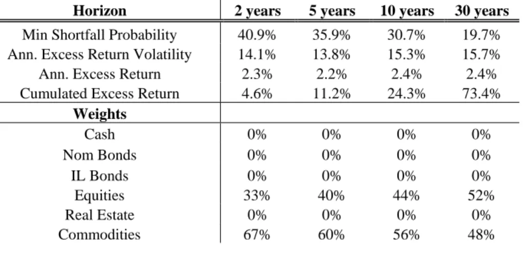
Min Shortfall Probability 40.9% 35.9% 30.7% 19.7%
Ann. Excess Return Volatility 14.1% 13.8% 15.3% 15.7%
Ann. Excess Return 2.3% 2.2% 2.4% 2.4%
Cumulated Excess Return 4.6% 11.2% 24.3% 73.4%
Weights Cash 0% 0% 0% 0% Nom Bonds 0% 0% 0% 0% IL Bonds 0% 0% 0% 0% Equities 33% 40% 44% 52% Real Estate 0% 0% 0% 0% Commodities 67% 60% 56% 48%
Table 12: Minimum shortfall probability portfolio, real return target 4%, January 1973-December 1990
Horizon 2 years 5 years 10 years 30 years
Min Shortfall Probability 44.0% 41.5% 37.8% 29.9%
Ann. Excess Return Volatility 21.3% 18.1% 18.1% 18.4%
Ann. Excess Return 2.3% 1.7% 1.8% 1.8%
Cumulated Excess Return 4.5% 8.6% 17.7% 53.1%
Weights Cash 0% 0% 0% 0% Nom Bonds 0% 0% 0% 0% IL Bonds 0% 0% 0% 0% Equities 0% 14% 23% 32% Real Estate 0% 0% 0% 0% Commodities 100% 86% 77% 68%
Table 13: Minimum shortfall probability portfolio, real return target 0%, December 1990- June 2009
Horizon 2 years 5 years 10 years 30 years
Min Shortfall Probability 4.7% 3.2% 1.3% 0.0%
Ann. Excess Return Volatility 1.3% 3.0% 4.8% 5.1%
Ann. Excess Return 1.5% 2.4% 3.4% 3.2%
Cumulated Excess Return 3.0% 12.2% 33.8% 96.7%
Weights Cash 80% 41% 0% 0% Nom Bonds 17% 48% 77% 73% IL Bonds 0% 0% 0% 0% Equities 0% 5% 10% 10% Real Estate 1% 0% 0% 0% Commodities 2% 6% 13% 17%
Table 14: Minimum shortfall probability portfolio, real return target 1%, December 1990-June 2009
Horizon 2 years 5 years 10 years 30 years
Min Shortfall Probability 16.0% 9.1% 5.8% 0.8%
Ann. Excess Return Volatility 4.5% 4.5% 4.8% 5.3%
Ann. Excess Return 3.2% 2.7% 2.4% 2.3%
Cumulated Excess Return 6.3% 13.3% 24.1% 70.2%
Weights Cash 0% 0% 0% 0% Nom Bonds 76% 78% 76% 69% IL Bonds 0% 0% 0% 0% Equities 17% 13% 10% 10% Real Estate 0% 0% 0% 0% Commodities 7% 10% 14% 21%
Table 15: Minimum shortfall probability portfolio, real return target 2%, December 1990-June 2009
Horizon 2 years 5 years 10 years 30 years
Min Shortfall Probability 24.7% 20.6% 17.4% 7.5%
Ann. Excess Return Volatility 4.5% 4.6% 5.1% 6.4%
Ann. Excess Return 2.2% 1.7% 1.5% 1.7%
Cumulated Excess Return 4.4% 8.4% 15.1% 50.4%
Weights Cash 0% 0% 0% 0% Nom Bonds 75% 76% 72% 60% IL Bonds 0% 0% 0% 0% Equities 18% 13% 9% 9% Real Estate 0% 0% 0% 0% Commodities 7% 11% 19% 30%
Table 16: Minimum shortfall probability portfolio, real return target 3%, December 1990-June 2009
Horizon 2 years 5 years 10 years 30 years
Min Shortfall Probability 35.4% 36.4% 34.1% 18.8%
Ann. Excess Return Volatility 4.7% 5.1% 9.9% 18.9%
Ann. Excess Return 1.2% 0.8% 1.3% 3.0%
Cumulated Excess Return 2.5% 3.9% 12.8% 91.5%
Weights Cash 0% 0% 0% 0% Nom Bonds 73% 69% 42% 0% IL Bonds 0% 0% 0% 0% Equities 20% 11% 0% 0% Real Estate 1% 5% 7% 0% Commodities 5% 15% 51% 100%
Table 17: Minimum shortfall probability portfolio, real return target 4%, December 1990-June 2009
Horizon 2 years 5 years 10 years 30 years
Min Shortfall Probability 44.9% 45.9% 41.3% 27.6%
Ann. Excess Return Volatility 12.5% 16.3% 18.3% 18.9%
Ann. Excess Return 1.1% 0.7% 1.3% 2.1%
Cumulated Excess Return 2.3% 3.7% 12.8% 61.6%
Weights Cash 0% 0% 0% 0% Nom Bonds 26% 0% 0% 0% IL Bonds 0% 0% 0% 0% Equities 33% 0% 0% 0% Real Estate 40% 54% 0% 0% Commodities 0% 46% 100% 100%