HAL Id: dumas-02946542
https://dumas.ccsd.cnrs.fr/dumas-02946542
Submitted on 23 Sep 2020HAL is a multi-disciplinary open access archive for the deposit and dissemination of sci-entific research documents, whether they are pub-lished or not. The documents may come from teaching and research institutions in France or abroad, or from public or private research centers.
L’archive ouverte pluridisciplinaire HAL, est destinée au dépôt et à la diffusion de documents scientifiques de niveau recherche, publiés ou non, émanant des établissements d’enseignement et de recherche français ou étrangers, des laboratoires publics ou privés.
Reconstruction of high-resolution 3D models using
MPCD technique to study local changes on the surface
of comet 67P
Raghav Awasty
To cite this version:
Raghav Awasty. Reconstruction of high-resolution 3D models using MPCD technique to study local changes on the surface of comet 67P. Astrophysics [astro-ph]. 2019. �dumas-02946542�
RECONSTRUCTION OF
HIGH-RESOLUTION 3D MODELS USING
MPCD TECHNIQUE TO STUDY LOCAL
CHANGES ON THE SURFACE OF
COMET 67P
Raghav Awasty (M2 FunPhys Master, 2018-19)
Under the supervision of Laurent Jorda1
Acknowledgements
This work was done using the services provided by the Laboratoire d’Astrophysique de Marseille.
I would like to thank my supervisor, Laurent Jorda, for his encouragement and motivating words at every step of the work. My interactions and discussions with him made the internship quite exciting.
I also want to thank my family for their support without which I would not have the opportunity to be here.
Lastly, I thank my colleague, Pooja Sharma, who was constantly pushing me to solve any problems I faced and kept me motivated through the internship.
2
Table of Contents
1. Introduction 3 1.1. Rosetta 5 1.2. Comet 67P/Churyumov-Gerasimenko 7 2. 3D reconstruction 10 2.1. MPCD technique 11 2.1.1. Input Model 13 2.1.2. Image Selection 13 2.1.3. Optimization 183. Boulder Characterization from optimized DTMs 24
3.1. Position Estimation 24
3.2. Dimension Estimation 26
3.3. Volume Estimation from DEM 27
4. Dynamic Models 30
4.1. Light received by local area 30
4.2. Surface Temperature 33
4.3. Water production rate 34
4.4. Non-gravitational acceleration 34
5. Results 35
5.1. Scenario 1 - Periodic Bursts 35
5.1.1. Movement of boulder 36
5.2. Scenario 2 - Single Outburst 38
5.2.1. Movement of boulder 38
5.3. Minimum surface fraction required 39
5.4. Summary 39
6. Conclusions 41
7. Bibliography 43
3
1. Introduction
Being one of the oldest bodies in our Solar System, comets hold the key to answering questions about the formation and the evolution of the Solar System. In the last couple of decades, a large number of comets have been categorized through various missions such as Deep Space 1, Deep Impact, Rosetta etc.
Our Solar System formed from a cloud of gas and dust, spanning several light years across, about 4.6 billion years ago. The gas and dust were gravitationally pulled into the rotating core where it was concentrated and eventually formed the Sun, leaving behind a disk of material at the core’s equator. This material collated to form the planets within the next few million years. Additionally, the ‘left over’ material formed smaller bodies of frozen dust and gas in the outer Solar System because of the cold temperatures.
The evolution of the Solar System was strongly influenced by planetary migration, described by the ‘Nice model’. According to it, the Kuiper belt was much denser and existed much closer to the Sun. Interactions with small bodies caused the orbits of giant planets to change, leading to the movement of Jupiter and Saturn inwards into the Solar System which destabilizing the orbits of Neptune and Uranus causing them to switch places and move outwards. The movements of these planets resulted in their interaction with the planetesimals causing them to scatter. Some were flung towards the inner planets resulting in the late heavy bombardment event and others were sent outwards into very elliptical orbits (forming the Oort cloud) or ejecting them out of the Solar System. Comets are icy bodies that are segregated into 3 parts: the nucleus, coma and tail. The nucleus is the solid core structure of the comet having a dry rocky surface with ice hidden beneath it. The ices content is dominated by water ice, but the nucleus also contains frozen gases such as carbon monoxide, methane, carbon dioxide, ammonia, etc. As the comet approaches the sun during its orbit, the ice beneath the surface starts sublimating through a process called outgassing. This leads to the ejection of dust and the trapped gasses which produce the coma that envelopes the nucleus. The characteristic tail of comets is also composed of these ejected materials created by the forces exerted by the solar radiation and solar wind and because of this, points away from the sun. Tails contain dust and ionized molecules each forming their individual tails. The dust consists of small particles and forms a curved, diffuse tail. The interaction of the UV radiation from the sun causes ionization of the particles from the coma forming a straight outward pointing tail. Comets have elliptical orbits and can be classified based on the eccentricity of their orbits (Eicher, 2013). Short period comets have an orbital period of 200 years or less with orbits originating from the Kuiper belt (Halley’s comet is an interesting short-period comet with
4
a period of 76 years, originally originating from the Oort cloud) just beyond Neptune. These are also further classified into a ‘family’ or ‘type’ depending on the closest planet to their aphelia. The shortest period comets, with orbits not reaching Encke-type comets. Comets with a period of less than 20 years are called Jupiter-family comets and can have up to 30 degrees inclination from the ecliptic. Finally, comets with periods between 20 and 200 years and inclination up to 90 degrees are called Halley-type comets. The second type of comets are called Long Period comets with periods ranging from 200 years up to millions of years. These comets originate from the Oort cloud which lies at the outer edge of the Solar System.
There have been many space missions to explore and characterize comets in order to understand the clues they hold about the evolution of the Solar System. An overview of the major past missions is provided in Table 1:
Mission Year Space Agency Comet International Cometary
Explorer (ICE) 1978 NASA/ESA 21P/Giacobini–Zinner Vega 1 and Vega 2 1984 IKI (Russia) 1P/Halley Sakigake and Suisei 1985 ISAS (Japan) 1P/Halley
Giotto 1985 ESA 26P/Grigg–Skjellerup 1P/Halley and Deep Space 1 1998 NASA 107P/Wilson–Harrington and 19P/Borrelly
Stardust 1999 NASA 81P/Wild and 9P/Tempel Rosetta 2004 ESA 67P/Churyumov–Gerasimenko Deep Impact 2005 NASA 9P/Tempel and
103P/Hartley
Table 1: Overview of past space missions to comets
These missions have been widely successful in categorizing many comets. ICE was the first spacecraft to visit a comet as it passed through the ion tail of comet 21P/Giacobini-Zinner and was successful in providing the first in situ measurements of the magnetic field and environment of a comet’s tail.
Subsequent missions in 1986 were targeted on Halley’s comet. Suisei and Sakigake were instrumental in imaging the coma as well as making measurements on the solar winds and the energetic particle environment ahead of the comet. The Vega spacecrafts both flew through the Halley coma to make various measurements on the gas and dust
5
composition as well as the magnetic field. This was also the first time a picture of a cometary nucleus was obtained. Giotto added to these achievements by returning the highest-resolution images of the nucleus showing more detailed features of the terrain. These missions were also successful in identifying the gasses and elements that the comet was composed of.
A decade later, NASA’s Deep Space 1 mission was launched which images and characterized the nucleus of 19P/Borrelly. The following year, Stardust was launched which became the first mission to collect and return dust samples from comet 81P/Wild back to Earth. Images from Stardust also showed a surface that was very different from previously observed comets. Deep Impact was the last mission to be launched by NASA in 2005. Targeted at comet 9P/Tempel 1 it carried a spacecraft for flyby and an impactor to study impact craters and provided the highest resolution images of the surface ever obtained. The dust ejected from the impacted was used to model the gravity of the nucleus making it possible for the first time, for the mass and density of a nucleus to me measured. The spacecraft also did a flyby of 103P/Hartley observing its unique complex rotation and activity.
The European Space Agency (ESA) launched Rosetta in 2004 with the goal of studying the comet 67P/Churyumov–Gerasimenko (hereafter ‘67P’). On its way to 67P, Rosetta also gathered significant data on asteroids 2867 Steins and 21 Lutetia. These missions have significantly enhanced our understanding on comets, their composition and their dynamics. For the purpose of this study we focused on the observation by the Rosetta mission of comet 67P.
1.1. Rosetta
The Rosetta mission launched by ESA in 2004 made history as the first spacecraft to orbit and land an instrument on a comet. It was targeted to rendezvous with 67P and continue to escort it along its orbit around the Sun. The main objectives of this mission were to better understand the origins of comets and their evolution as they interact with interstellar material and to unravel the clues about the origins of the Solar System. To accomplish these goals the spacecraft needed to complete measurements such as (http://sci.esa.int/rosetta/):
Characterizing the global properties of the nucleus such as surface morphology and its dynamic properties.
Studying the chemical composition and physical properties of volatiles and refractories in a comet’s nucleus.
6
The Rosetta spacecraft carried onboard a host of instruments. The orbiter carried 11 instruments (e.g. MIDAS, MIRO, OSIRIS etc.) to perform imaging at various wavelengths, spectrometry of dust and gas particles and to study solar wind interaction. Marking an exceptional achievement, the orbiter became the first spacecraft to provide a complete view of a comet by orbiting around it. This allowed the acquisition of data about the activity and its evolution as the comet made its approach to the Sun, right up to the perihelion and then as it went away from the Sun moving to the outer Solar System. It also offered a unique opportunity to map the surface of the nucleus in high detail.
Figure 1: The Rosetta spacecraft and Philae lander with 67P. Image Credit: ESA/Getty Images
Rosetta also carried a lander module called Philae which had its own set of 10 instruments focused on studying the composition of the cometary materials and performing experiments to characterize the physical properties of the materials on and below the surface. Philae landed successfully (albeit not exactly as planned) on the surface of 67P on 12th November 2014.
Data from SESAME (Surface Electrical, Seismic and Acoustic Monitoring Experiment) revealed information about the diversity of the surface which was previously believed to be homogeneously soft (Boehnhardt, 2017). While the surface of the initial landing site was relatively soft, the final site’s surface was much harder. The CIVA (Comet Infrared and Visible Analyzer) camera captured images showing a fractured surface scattered with
7
boulders and a variety of reflectivities that further highlighted the complexity of the surface (Bibring et al., 2015a). Philae was also equipped with the ability to drill into the surface to provide soil samples for in situ analysis by the PTOLEMY and COSAC (Cometary Sampling and Composition) instruments. COSAC detected 16 compounds out of which four (acetamide, methyl isocyanate, propionaldehyde, and acetone) had never been detected on any comet before making this a very exciting result (Bibring et al., 2015b). The Rosetta spacecraft made its way through a 10-year journey to 67P in 2014 and continued to escort the comet until its perihelion in 2015. During this period the Philae craft landed on the surface in November 2014. Post-perihelion, Rosetta continued to orbit 67P as it made its way to the outer Solar System until the end of the mission in September 2016.
1.2. Comet 67P/Churyumov-Gerasimenko
67P is a short-period comet belonging to the Jupiter family of comets. It is a regular visitor to the inner Solar System with an orbit period of 6.5 years (Lamy et al., 2007). It was discovered by Klim Ivanovic Churyumov and Sveltana Ivanova Gerasimenko at Alma-Ata Observatory, Russia in 1969.
8
Jorda et al. (2016) performed a high-resolution reconstruction of the comet surface using stereophotoclinometry (SPC) method developed by Gaskell et al. (2008a) to obtain a model of the comet and characterize its properties. The bilobed shape of the comet was used to estimate the volume of the comet to be 18.8 0.3 km3 with a mean radius of
1.743 0.007 km and a density of 532 7 kg m-3. Deriving the density also gave insight
into the very high porosity of the aggregated material to be about 70 - 75% suggesting the presence of large-scale voids in the internal structure of the nucleus.
Using light curves from observations since 2003, Lamy et al. (2007) deduced the spin period of the comet to vary between 12.4 and 12.7 hours. Later, Mottola et al. (2014) used another set of light curves from the OSIRIS instrument obtained during the comet’s perihelion passage in 2009. These observations indicated a reduction in the spin period from 12.7 to 12.4 hours. This value increased and reached a maximum of 12.43 hours in May 2015 and started dropping rapidly just before the perihelion in August 2015 until finally converging post-perihelion to 12.07 hours in December 2015 (Jorda et al., 2016). This variation (Fig. 3) is explicable by the thermal model by Keller et al. (2015). This clearly shows a trend that the comet spin period is decreasing by 0.3 hours with each perihelion passage. This can be explained by the torque created by the recoil force being caused by the outgassing process.
Figure 3: Variability of spin period of 67P close to perihelion (data from R. Gaskell obtained through personal communication by L. Jorda)
9
Date of discovery 20th September 1969
Orbital characteristics
Orbital period 6.45 years Perihelion distance 1.243 AU
Aphelion distance 5.68 AU Spin axis RA: 69.57 0.35°
Dec: 64.01 0.12° Physical characteristics Mean radius 1.743 0.007 km Mass 1 1013 kg Volume 18.7 km3 Density 533 6 kg/m3
Spin period 12.06 (September 2016) Porosity 70 – 75%
Albedo 6%
Table 2: Orbital and Physical characteristics of 67P (Jorda et al., (2016); ESA)
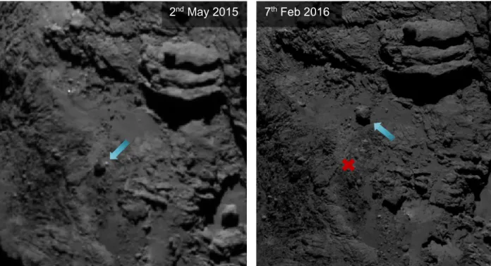
As seen above, the properties of 67P (summarized in Table 2) have been strongly characterized through various studies. However, to identify and understand in-depth the processes that are responsible for the activity on the nucleus, there is a need to study locations where surface changes takes place and explain those changes. The purpose of this study is precisely that. The aim was to study a local section of the surface of 67P, the Khonsu region in the southern/equatorial area, where a large boulder was observed to have moved in the images taken before and after perihelion (Fig. 4).
10
Figure 4: Left: Boulder location pre-perihelion, Right: Boulder location post-perihelion (X marks the original position); Blue arrow marking the position of the boulder
The following sections describe the work done in this study. Section 2 describes the process of 3D reconstruction that was essential to characterize the aforementioned boulder and study the changes. In section 3, the method used to characterize the boulder and its various properties are explained. These measurements were then used to study the dynamic scenario that potentially resulted in the observed changes and are described in section 4. Finally, in section 5 the results of this study are presented and discussed with final conclusions in section 6. We pose the questions: “Is it realistic to explain the displacement of the boulder by the outgassing of an ice pocket at its surface?”.
2. 3D reconstruction
3D reconstruction methods have been extensively used to obtain accurate models of comets and asteroids and study their properties since the Vega and Giotto satellites acquired the first images of the comet 1P/Halley. Different methods have been developed and implemented in the past to perform reconstruction but today, they can be separated into two categories: stereophotogrammetry (SPG) and stereophotoclinometry (SPC). SPG involves extracting information about the three-dimensional coordinates of a point using multiple image patches taken from different locations. It uses the line of sight to triangulate the coordinates and has been established to produce accurate models since it only deals with the geometry. It can also work between images of the same location
11
that may be geometrically different (transformations like rotation, translation etc.). Conversely, SPC is a method developed by Gaskell et al. (2008b), that uses the relative intensities of pixels and reference heights from stereo to construct a map representing the elevation of the surface. It uses several images of an area taken from different points of view and illumination conditions to perform the reconstruction. This method is restricted by the illumination parameters and the positions of the light source and the observer. In unfavorable illumination conditions, SPC tends to smooth out small topographical features. Moreover, areas in shadows are reconstructed poorly. Additionally, a method that has been recently developed by Capanna et al. (2013) known as Multi-resolution PhotoClinometry by Deformation (MPCD) (section 2.1.) combines features of both SPG and SPC. This is the method that has been used in this study to reconstruct the local 3D models.
2.1. MPCD technique
This method works by taking an input 3D mesh (section 2.1.1.) with triangular faces (Fig. 5) and running it through a non-linear optimization process (section 2.1.3.) with the aim of minimizing the chi square differences between the model and the observed images (section 2.1.2.).
Figure 5: Wireframe of the mesh showing the triangular faces
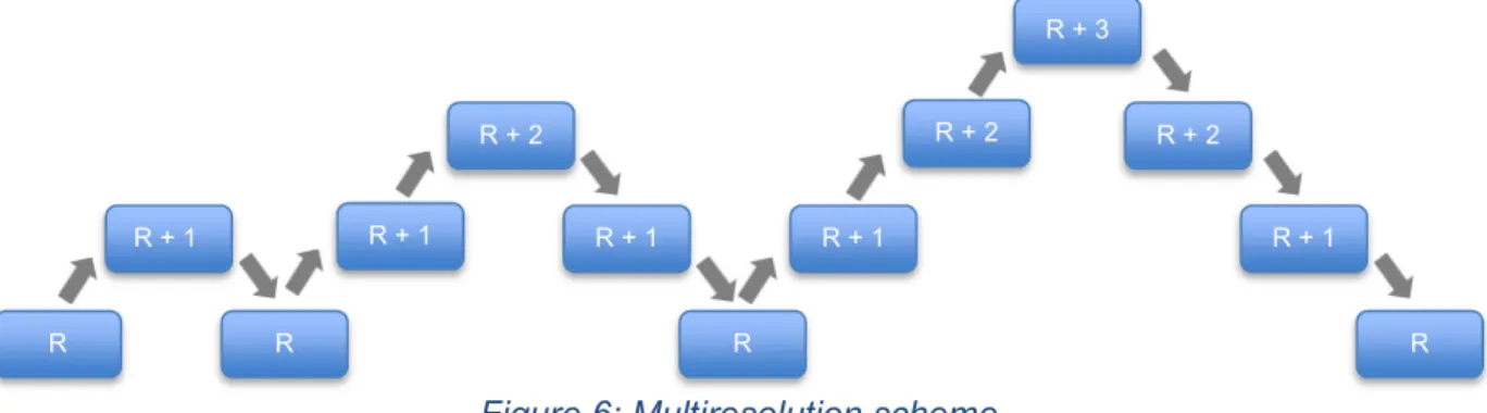
Synthetic images are created from the mesh and the mesh is deformed until the difference between the observed and synthetic images is minimized. This deformation employs a “Full multigrid” multiresolution scheme (Fig. 6) wherein the resolution of the mesh and the
12
pixel scale of the images change through the optimization process. For a resolution ‘R+1’, the scheme goes to the lowest resolution ‘R’ through each intermediate level of resolution and then moves back to resolution ‘R+1’ again through the intermediate levels. It then moves up another level of resolution to ‘R+2’ repeating the process with each iteration. Hence, the name Multiresolution PhotoClinometry by Deformation.
The MPCD method (displayed in Fig. 7) works in the following steps:
The chi-square differences between the synthetic and observed images are computed using a maximum likelihood estimation.
A deformation is applied onto the mesh in order to minimize the differences. Optimization: the chosen algorithm (section 2.1.3.) maximizes the likelihood. The multiresolution scheme is applied.
Figure 7: Flow chart of the MPCD method
R R + 1 R R + 1 R + 2 R + 1 R R + 1 R + 2 R + 3 R + 2 R + 1 R
13
2.1.1. Input Model
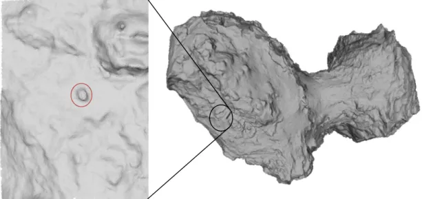
The MPCD method makes use of a 3D triangular mesh as in input model. This model is a low-resolution model that can be obtained from other methods. The 3D mesh of the global shape of the nucleus of 67P has been obtained from a colleague, R. Gaskell. Since this study is focused only on a local area the first step is to extract this portion of the mesh as a squared digital terrain model (DTM) which will be referred to as a ‘maplet’ (Fig. 8).
The extraction of the DTM was done using the tools available in the software “MeshLab” (Cignoni and Ranzuglia, 2011) and another software called “ReMESH” (Attene and Falcidieno, 2006) to create uniform subdivisions of the facets in the mesh. The extracted DTM is subject to adjustments based on the number of high-resolution images that are selected in the next step. The image selection (section 2.1.2.) happens in such a way that any images which do not contain the entire DTM area is rejected. Hence, there is a need to find the middle ground between the size of the DTM and the number of high-resolution images, which can lead to the gain or loss of a level of resolution.
2.1.2. Image Selection
As discussed before the MPCD reconstruction process requires both an input model as well as observed images. For acquiring the images showing the area, a software called ‘SUMXSEL’ was used. The software takes the DTM that was extracted as an input which provides the Sun-comet and comet-Sun vectors as well as the rotation matrix from the
Figure 8: Right panel: Global 3D shape model of 67P (boulder encircled), Left pane: Extracted DTM of local area
14
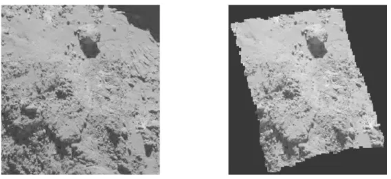
camera to the comet for the OSIRIS images. SUMXSEL then uses this information to compute the emission angle, phase angle and incidence angles of all the facets of the DTM for each image. The favorable range of these angles which would be useful for the reconstruction process are set beforehand in a parameter file along with the start and end date between which the images taken are considered. As the software goes through the images falling within the time range it selects the images that fulfils all the conditions and creates a mask of the DTM area on the image (Fig. 9).
Figure 9: Left: Original image, Right: Image with mask of DTM area
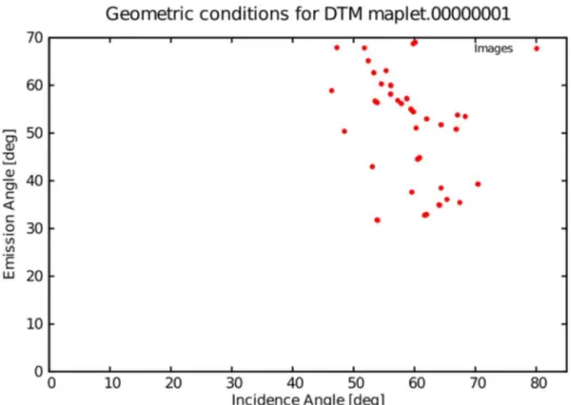
The selection process can return more than 500 images out of the available 30000 OSIRIS narrow angle and wide-angle camera (NAC and WAC) images depending on the conditions and the DTM area. These first-selection images can be projected on a plot of incidence angle versus emission angle (Fig. 10) and are represented by the red dots.
15
As we can see there are a lot of images that are very close together. These are images that were taken by the satellite in small time intervals and therefore have very similar geometric conditions. Since such images will not contribute any additional information for the reconstruction process and will only end up increasing the computation time, the software rejects images with very similar geometric conditions and keeps the ones with a higher resolution (Fig. 11). This second step returns a maximum of 40 images. The final selected images are then sorted by the software into different levels based on their resolution.
Figure 11: Final selection by the SUMXSEL software refining the pre-selected image list
The reconstruction process depends strongly on this step of the image selection since a good distribution of the geometric conditions ensures that the area has been observed from various points of view and more information is available for a better reconstruction. However, that is not always the case and sometimes because of either the area of interest, the extraction of the DTM or the OSIRIS images available, the final selection from SUMXSEL might not be very promising. Such a case is shown in Fig. 12.
16
Figure 12: Unfavorable geometric conditions: images with similar incidence and emission angles
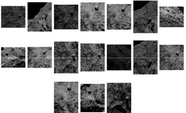
The final selected images are shown below:
Figure 13: Final image list after selection by SUMXSEL
Once this automated step is complete, there is a need of performing a final manual inspection. This step is required to remove any images that have made it through the final selection of the SUMXSEL software but may possess certain instrumental errors or post processing issues such as:
17
Shadows cast on the area to be reconstructed by external topography (Fig. 14(a)) Blurring of image
Saturation of image (Fig. 14(b))
(a) (b)
Figure 14: Left top: Original image, Left bottom: Image with mask of DTM area with shadow cast from outside, Right: Saturated image
In some cases, the image might be a good one because of its high resolution, making it essential for a good reconstruction, but it might have a bright spot due to specular reflection that would introduce inaccurate artifacts in the final reconstruction. This can be dealt with by creating a mask that removes the bright spot (Fig. 15) therefore, all information except the bright spot is taken into account during the MPCD reconstruction.
18
This step of manual selection must be done with caution for two reason:
To ensure that there are at least of 12 - 15 images for the MPCD algorithm to reconstruct the model accurately.
To ensure no less than 3 images at the last resolution as these images will most affect the accuracy of the model.
After this step a final list of images (Fig. 16) is obtained which are free of any features that may hinder the reconstruction process. As seen below, the images that were either covered in shadow from external topography or saturated images have been removed.
Figure 16: Final images after manual selection
2.1.3. Optimization
Once the image selection is done, we can then move on to the optimization. For this step, we used the services of the cluster at LAM which allows the algorithm to run in parallel in order to achieve faster computation time.
The optimization process uses a maximum likelihood estimation to minimize the difference between the synthetic images (created from the 3D mesh) and the observed images. We have a function F that is minimized:
19
Where,
𝐿(𝑝 ) = (𝑂 − 𝑆 (𝑝 )) 𝜎 (𝑝 )
Is the non-linear maximum likelihood function of the free parameters (pk) and quantifies
the differences between the observed images (O) and the synthetic images (S). These differences are used to apply the deformation of the mesh by shifting the vertices along the normal. In order to ensure that the deformations that are applied produce accurate topographic features and do not introduce artifacts, it is important to make sure that the deformation of one vertex does not directly influence the deformation of its surrounding vertices. For this reason, a smoothness parameter (SC) is applied during the maximum
likelihood estimation which forces the slope of the surrounding facets to remain close from each other. The smoothness parameter is computed for each vertex by taking the normal of the facets which share that vertex.
Depending on previous factors, the deformation of the 3D mesh is done by changing the height of each vertex along a normal vector which is calculated for each vertex by taking the average of each facet sharing this vertex. The optimization process applies a non-linear method based on a quasi-Newton large scale minimization algorithm, “L-BFGS-b” (Morales et al., 2011). Although, there are other methods available, Capanna et al. (2013) found L-BFGS-b to be the best method for minimizing the function. One key factor of this method is that it will only converge to a global minimum if the function being minimized is a convex function.
Finally, the multiresolution scheme (Fig. 6) is applied. This helps in overcoming a key obstacle which is that the function may not always be convex therefore, the optimization process will not converge to a global minimum but only a local one. This scheme allows the minimization algorithm to leave the local minima by first using the low-resolution images to recreate larger features and then moving to higher resolutions to bring out more detailed features, removing the local minima and eventually reaching to the global minimum.
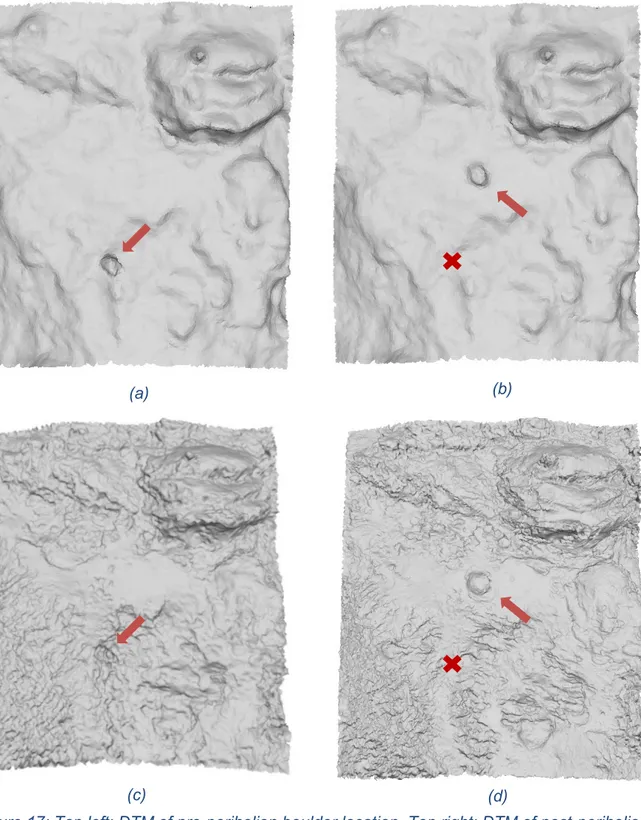
Taking all the above factors in consideration, the optimization process is applied to the DTM. After each optimization iteration, an image simulator tool called OASIS (Optimized Astrophysical Simulator for Imaging Systems) developed by Jorda et al. (2010), is used to generate a set of synthetic images from the shape model. This complete optimization process of MPCD has been applied on the section of the comet containing the boulder shown in (Fig. 8). This site was reconstructed for two different time periods, one before the perihelion and one after (Fig. 17), which allows us to study the evolution.
20
We noticed that the first reconstruction with a smoothness parameter of 750 was creating high-frequency artifacts (which look like folds or waves on the surface) in the output model. To reduce this the smoothness parameter would have to be changed which would
(b) (a)
(c) (d)
Figure 17: Top left: DTM of pre-perihelion boulder location, Top right: DTM of post-perihelion boulder location, Bottom left: Reconstructed DTM (Pre-perihelion), Bottom right: Reconstructed
21
also lead the chi-square value to change. To constrain the optimum value of the smoothness parameter for which the chi-square value would be the least, we tried the reconstruction with several value, tracking the variation of the chi square values with the smoothness parameter (Fig. 18).
Figure 18: Variation of chi-square value with smoothness parameter
It can be seen from the plot that the for a smoothness of ~4000, we get the best value for the final chi-square. The reconstruction for the DTM was performed again with the optimum smoothness value (Fig. 19(b)) and this value was kept constant for the reconstruction of other DTMs. The reconstructed DTMs are presented in Table 3.
Figure 17(c) 17(d) / 19(a) 19(b) 20(c) 20(d)
DTM Pre-perihelion Post-perihelion Post-perihelion Pre-perihelion Post-perihelion
Date 15/07/2014 – 15/06/2015 01/12/2015 – 30/09/2016 01/12/2015 – 30/09/2016 15/07/2014 – 15/06/2015 01/12/2015 – 30/09/2016 No. of levels 2 3 3 2 4 Smoothness 750 750 4000 4000 4000 Chi-square 3014 4494 3782 738 1464 Initial1 facets 22188 22182 22182 3809 3633
22 Final facets 355008 1419648 354912 15236 232512 Initial surface (m2) 563637 563557 563557 96937 92527 Final surface (m2) 690589 701547 630960 101839 102650 Initial resolution (m) 5.040 5.040 5.040 5.044 5.046 Final resolution2 (m) 1.395 0.703 1.333 2.585 0.664
Quality Medium (some artifacts) Good (some artifacts) Very good Medium Very good
Table 3: List of DTMs reconstructed by MPCD
We see that the reconstruction with the optimum smoothness value produces much less artifacts and gives a much better chi-square value. However, because of the area contained in the DTM itself, the reconstruction was still not ideal. Particularly, because of the presence of the big rock (jokingly called the ‘hotdog’ rock) the MPCD algorithm could not refine the smaller features of the boulder more accurately. To tackle this, the DTM was further modified to only contain the area where the boulder was situated and the reconstruction was done for these DTMs (Fig. 20).
2 The resolution is given by: 𝑅 = 𝑆𝑢𝑟𝑓𝑎𝑐𝑒 𝐹𝑎𝑐𝑒𝑡𝑠⁄
Figure 19: Comparison between reconstructed DTM (Post-perihelion), Left: Smoothness: 750, Right: Smoothness: 4000, Boulder position marked with arrow, original location marked with X
23
(b) (a)
(c) (d)
Figure 20: Smaller DTM of boulder location, Top left: Pre-perihelion, Top right: Post-perihelion, Bottom left: Reconstructed (Pre-perihelion), Bottom right: Reconstructed
24
Indeed, the reconstruction of the smaller DTMs (Fig. 20) is much better than the bigger models with a better value for chi-square (refer to Table 3). The pre-perihelion (Fig. 15(a), 15(c)) model does not seem to be ideally reconstructed. This is because of the absence of high-resolution images as the satellite started to move away from 67P before it approached its perihelion. However, the reconstruction of the post-perihelion DTM (Fig. 15(b), 15(d)) is very remarkable. Using this model, we have tried to characterize the boulder in order to be able to study its movement and quantify the dynamics behind this change.
3. Boulder Characterization from optimized DTMs
In order to study the non-gravitational forces that led to the movement of the boulder from its original location during the perihelion, it is important to first accurately characterize the boulder and obtain the parameters that drive these changes. This is done by using both the observed images of the area acquired by the SUMXSEL software and the optimized DTMs. Mainly, the parameters required to study the dynamics were:
The position of the boulder to quantify the amount of distance that it had moved. The dimensions of the boulder to compute its volume and mass for the calculation
of the non-gravitational forces.
3.1. Position Estimation
The first step in the estimation of the position of the boulder in both the pre-perihelion and post-perihelion time period was to find out the coordinates of its center of mass. To make sure the estimation was as accurate as possible, this was done by two different methods and later cross correlated.
The first method, although not very rigorous, gives a good first approximation for the center. From the optimized DTM, using the selection tool in MeshLab, a facet is selected (Fig. 21) which appears to be at the center of the boulder’s surface. The information about the coordinates of the vertices of the selected facet is obtained and the center of the facet is computed by averaging the coordinates. This process is repeated for a few more surrounding facets which occupy the central zone of the boulder’s surface. Finally, the total average is computed which gives the estimate of the coordinates of the center (Table 4). This process is done for both the post-perihelion and post-perihelion DTMs.
25
Figure 21: Boulder model with central facet selected and showing coordinated (zoomed in)
In the second method, we used the DTMs to extract only the facets that make up the boulder (Fig. 22). The information about the coordinates of the vertices of these extracted facets is stored in a separate file. These coordinates are then used to estimate the coordinates of the geometric center of the boulder by averaging all the vertex coordinates. This gives a second estimate for the center of mass and very closely matches the value from the first method (Table 4).
Figure 22: Extracted boulder facets
Once we have the values of the coordinates of the center of mass for pre-perihelion and post-perihelion boulder positions, we can use them to compute the distance between the two. Using this process, the distance that the boulder had moved during the perihelion
26
was found to be approximately 178 1 m. This was further corroborated by using the measuring tool in MeshLab which gave a value of 175 1 m. We went with the value of 178 1 m since it was computed with a more robust method. This is a slightly higher value as compared to 140m estimated by El-Maary et al. (2017).
3.2. Dimension Estimation
Next, we move on to estimating the dimensions of the boulder. Again, two separate methods were applied to estimate the dimension to substantiate the results.
In the first method, we used the measuring tool in MeshLab to measure the length and width of the boulder from the optimized DTMs. Estimating the height is challenging due to the reconstruction process smoothing the edges which hides the elevation of the boulder from the surrounding surface and would not yield accurate results. For this step we only made use of the DTMs reconstructed for the post-perihelion period. This is because the optimizations for these DTMs gave a much better reconstruction of the boulder shape as compared to the pre-perihelion DTM (Fig. 20) and would therefore give a more exact representation of the dimensions. We measured a value of 36.9 0.5 m and 29.0 0.5 m for the length and width respectively.
In the second method, we used the images acquired by the SUMXSEL software to measure the number of pixels across the length and the width of the boulder. This was done using the ‘ruler’ tool in the software ‘fv’ which is a FITS file viewer and editor developed by NASA’s High Energy Astrophysics Science Archive Research Centre (HEASARC). The FITS images also contain information about the image acquisition such as the altitude of the spacecraft at the time of imaging and the pixel size. Using this information, the number of pixels of length and width can be converted to the actual dimensions of the boulder. Going through all the images these measurements can be validated for their accuracy. This resulted in a value of 37.4 0.8 m and 29.4 0.8 m for the length and width. These values are in agreement with the results from the first method. Additionally, the second method could also be used to estimate the height of the boulder. We can see the shadow being cast by the boulder in the images (Fig. 23). Since the longest part of the shadow is cast by the highest point of the boulder, we could measure the length from the longest edge of the shadow to the edge of the boulder and using the elevation angle of the sun, estimate the height by simple trigonometry. It is important however, to make sure that the measurement is done along the sun-comet vector so as to not overestimate the height.
27
As mentioned in section 2.1.2., SUMXSEL retrieves this information about the image. Using the sun-comet vector we can find the azimuth angle of the sun and rotate the image (Fig. 23) accordingly to have the shadow oriented vertically. This will ensure the measurement is exactly along the vector and does not overestimate the number of pixels.
Figure 23: Left: Boulder its shadow, Right: Image oriented for shadow length measurement
Using this method, we estimated the height of the boulder to be 25.6 0.8 m. By our estimation the boulder measure (25.6 0.8) m x (29.4 0.8) m x (37.4 0.8) m. Again, comparing to the values by El-Maary et al. (2017) of 20m x 30m x 40m our results show a slight disparity.
3.3. Volume Estimation from DEM
Apart from a basic calculation of the volume assuming an ellipsoid shape (28053 1340 m3) from the dimensions found above, we also applied a more rigorous method to
estimate the volume. Using the facets from the 3D mesh, a digital elevation model (DEM) can be generated. A DEM is a representation of the surface of a terrain. By using the normal vectors of the facets of the mesh an average normal is computed. This normal is assigned to a plane onto which, an orthogonal projection is done. The surface is divided in to a regularly sampled 2D grid and the elevation of each element is computed by bilinear interpolation3 using the stereo images. We generated the DEM for the optimized
DTM of the post-perihelion boulder location (Fig. 24).
28
Figure 24: Height map (DEM) of post-perihelion boulder position
This is a representation of the elevation of the boulder and its surrounding terrain. The DEM had a noticeable artifact in a few pixels during the interpolation process. This was corrected so as to reach a true approximation of the volume. The pixels’ data was replaced with an average value of intensity of the surrounding pixels (Fig. 25).
Figure 25: Corrected DEM
Next, to estimate the volume, the boulder needs to be extracted from the rest of the surface surrounding it. This is done by creating a mask around the boulder based on the intensity and removing the surrounding pixel values (Fig. 26).
29
Figure 26: Extracted boulder DEM
Once we have extracted the boulder, the intensity of each pixel along with the pixel size can be multiplied to find the volume of the entire boulder. We found a volume of 28557 1666 m3. As compared to the value by El-Maary et al. (2017) of 24000 m3 our results are
higher owing to the difference in dimensions. Using this result and the density (Table 2), the mass is also computed. The results of section 3 are summarized in Table 4.
Position
Pre perihelion Post perihelion First method -1.567, -0.642, -1.037 -1.631, -0.711, -0.885 Second method -1.560, -0.634, -1.029 -1.625, -0.704, -0.878 Distance (m) First method 178 1 Second method 178 1 3D Model 175 1
Dimensions (only from post-perihelion)
From 3D model From images
Length 36.9 0.5 Length 37.4 0.8 Width 29.0 0.5 Width 29.4 0.8 Height - Height 25.6 0.8 Volume (m3) From dimensions 28053 1340 From DEM 28557 1666 Mass (kg) (15.2 0.7) x 106
30
4. Dynamic Models
Using the characteristics of the boulder estimated in section 3, we then tried to model the forces that could possibly explain the changes during the perihelion period of 67P. This section describes the various steps in the modelling of the thermal dynamic processes that lead to the movement of the boulder. We assume that the motion of the boulder is due to outgassing from the surface of the boulder. This assumption is made based on the work by Desvoivres et al. (1999) where they modeled the dynamics of cometary fragments of similar size that were observed to be escaping from the nucleus in the dust tail of comet C/1996 B2 Hyakutake (Nakamura et al., 1996).
4.1. Light received by local area
The first step before diving into the calculation of the thermal processes was to find out how much sunlight does the boulder receive in one rotation of the comet. For this, we had to compute the elevation of the Sun from the boulder’s local frame. We started by obtaining the data about the ephemeris (tabulated information about the position) of the comet. This was done through the HORIZONS web interface tool developed by the Solar System Dynamics Group at NASA’s Jet Propulsions Laboratory (https://ssd.jpl.nasa.gov/horizons.cgi). The interface allows to set the target body, origin body and time period required. Using this we obtained a list of the Sun-comet vectors (SCEq(t)) between 1st June 2015 and 1st December 2015 (perihelion period) at intervals
of 15 minutes in the equatorial coordinate system in the J2000 reference frame.
The Sun-comet vectors were converted to comet-Sun vectors (CSEq(t)) by inverting them.
𝐶𝑆 (𝑡) = − 𝑆𝐶 (𝑡) 𝑆𝐶 (𝑡)
Following this the comet-Sun vectors had to be transformed from the equatorial frame (Eq) to the body fixed frame (BF) of the comet. To do this, the vectors had to be rotated by Euler angles. This is done by a sequence of rotations about the axes. We applied a ZXZ axis rotation with the θ, Φ, ψ Euler angles. According to this scheme the vector is first rotated about the Z-axis by an angle Φ, then about the X’-axis by and angle θ and finally about the Z’-axis by an angle ψ. The first two angles Φ and θ are constant and can be derived from the Right ascension (α) and Declination (δ) (refer to Table 2) of the comet and the third angle ψ is time dependent.
𝜃 =𝜋
2− 𝛿 𝜙 = 𝜋
31
Where:
ψ0 = 114.69° is the value of the zero-longitude taken from the Rosetta SPICE4
kernel files that contain the orientation constants of 67P (Scholten et al., 2015). ω is the time dependent spin period which was obtained from R. Gaskell (Fig. 3)
and interpolated to match the time step of the ephemeris being used.
These Euler angles are applied to the comet-Sun vectors (CSEq) in the aforementioned
ZXZ scheme by applying a rotation matrix, [REq→BF(t)] to get the comet-Sun vectors in the
body fixed frame (CSBF). This process is illustrated in Fig. 27.
[𝑅 → (𝑡)] = 𝑐𝑜𝑠(𝜓(𝑡)) −𝑠𝑖𝑛(𝜓(𝑡)) 0 𝑠𝑖𝑛(𝜓(𝑡)) 𝑐𝑜𝑠(𝜓(𝑡)) 0 0 0 1 × 1 0 0 0 𝑐𝑜𝑠(θ) −𝑠𝑖𝑛(θ) 0 𝑠𝑖𝑛(θ) 𝑐𝑜𝑠(θ) × 𝑐𝑜𝑠(𝜙) −𝑠𝑖𝑛(𝜙) 0 𝑠𝑖𝑛(𝜙) 𝑐𝑜𝑠(𝜙) 0 0 0 1 𝐶𝑆 (𝑡) = [𝑅 → (𝑡)] × 𝐶𝑆 (𝑡)
Figure 27: The ZXZ rotation scheme to change the vectors from equatorial to body fixed frame
Once the rotation matrix is used to transform the comet-Sun vectors from equatorial to body fixed frame of the comet, we can see how the elevation of the Sun changes through one rotation of the comet. The elevation of comet-Sun vectors is computed by taking the arctangent of the z and y-components of the vectors (Fig. 28(a)). We can see from Fig. 28 that the location of the boulder received sunlight for approximately half (~6.2 hours) of the rotation period. This information is important to know since the movement of the boulder can only be explained by the outgassing process happening which would produce the forces required to move the boulder. Outgassing can only occur when the boulder is exposed to the sunlight. A secondary check for the Azimuth angle of the Sun was also done to compare with the direction of motion (Fig. 28(b)).
4 ESA’s information system that uses ancillary data and provides Solar System geometry information for planning missions and analysing data. Developed and maintained by Navigation and Ancillary Information Facility (NAIF) team at the Jet Propulsion Laboratory (JPL).
32
Figure 28: Top: Elevation of the Sun from the boulder location through one rotation, Bottom: Variation of the Elevation of the Sun with the Azimuth
33
4.2. Surface Temperature
Knowing the amount of time for which the boulder receives the sunlight, we can study how it drives the temperature on the surface of the boulder. The surface temperature is required to estimate the water sublimation rate. The active regions of a comet have a surface temperature given by the surface energy balance (Maquet et al., 2012):
(1 − 𝐴 )𝐹ʘ
𝑟 𝑐𝑜𝑠 𝑧 = 𝜂𝜖𝜎𝑇 + 𝐿(𝑇)
𝑁 𝑍(𝑇) Where:
Ab = 0.06 is the bond albedo (product of phase integral and geometric albedo)
Fʘ = 1370 W m-2 is the solar constant at 1 AU5
rh is the time dependent heliocentric distance [AU] (||SCEq(t)||)
z is the time dependent elevation of the sun
η = 0.7 is the beaming factor introduced by Lebofsky et al. (1986) ϵ = 0.9 is the nucleus infrared emissivity
= 5.67 x 10⁻⁸ J K-4 m-2 s-1 is the Stefan-Boltzmann constant
T is the time dependent surface temperature [K]
L(T) is the latent heat of sublimation of water ice [J mol-1]
Na = 6.02 x 10²³ mol-1 is the Avogadro’s constant
Z(T) is the water sublimation rate [molecules s-1 m-2]
The latent heat of sublimation is given the following expressions where values have been obtained from Washburn (1928):
𝐿(𝑇) = (2740 + 2.01 − 0.014𝑇 + 0.00002𝑇 ) × 17.529929 The water sublimation rate is given by:
𝑍(𝑇) = (1 − 𝛼 )𝑃(𝑇) 1 2𝜋𝑀 𝑘𝑇 Where:
αR = 0.25 is the coefficient of recondensation on the surface of water ice (Crifo,
1987)
MH2O = 18 x 10-3 kgis the mass of water molecule
34
k = 1.38 x 10⁻²³ kg m2 s-2 K-1 is the Boltzmann constant
P(T) is the water saturation vapor pressure [Pa] given by Fanale & Salvail (1984): 𝑃(𝑇) = 𝐴 𝑒𝑥𝑝 −𝑇
𝑇
With A = 3.56 x 10¹² Pa and T0 = 6141.6607 K. Usually the temperature is a function of
both time and position (latitude and longitude), but since the boulder is such a small structure, we only take the time dependence into account. This allows then to estimate the temperature change as a function of time and through that, the water production rate.
4.3. Water production rate
From the surface temperature, we calculate the water production rate which is the amount of water molecules produced per second by outgassing. Only a fraction (f) of the surface is active and undergoes outgassing and the water production rate (QH2O) is given by:
𝑄 (𝑡) = 𝑆𝑓 (1 − 𝛼 )𝐴 𝑒𝑥𝑝 −𝑇 𝑇
𝑀 2𝜋𝑅𝑇 Where:
S is the total surface area of the boulder [m2]
f is the fraction of the surface which is active R = 8.314 J K-1 mol-1 is the gas constant
Finally, we can use this to compute the mass lost during each period of outgassing and incorporate that into the calculation of the non-gravitational acceleration.
4.4. Non-gravitational acceleration
Using the water production rate Maquet et al. (2012) defines the non-gravitational acceleration with Newton’s second law of motion as:
𝐴 (𝑡) = 1
𝑀 𝐶 𝑆 1
𝑃 𝑍 (𝑡)𝑉 (𝑡)𝑀 𝑁 𝑑𝑡′
The model proposed by Maquet et al. (2012) considers latitudinal bands along the surface of the nucleus with surface of band (Sj) and active fraction of band (Cj) and fits the
35
parameters depending on each band. However, in our study the boulder is much smaller in size and does not need to follow this model. Hence, we simplify the equation:
𝐴 (𝑡) = 1
𝑀 𝑓𝑆𝑍(𝑡)𝑉(𝑡)𝑀
Here Mb is the mass of the boulder (section 3.3.) and Z(t) is the sublimation rate (section
4.2.). V(t) is the thermal gas velocity [m s-1] proposed by Crifo (1987) given by:
𝑉(𝑡) = 𝜂∗ 8𝑘𝑇 𝜋𝑀
Here η* = 0.5 is a local parameter which takes into account the non-uniform smoothness
of the terrain. Using the above equations, we can compute the non-gravitational acceleration that the boulder experiences during the outgassing process.
5. Results
We propose two possible scenarios for the movement of the boulder. In the first case (section 5.1.), the outgassing process takes places from a very small area of the surface and the boulder requires multiple bursts to be able to cover the distance. In the second case (section 5.2.), the area of outgassing site is relatively larger and only one burst is sufficient enough for the boulder to cover the distance. We choose arbitrary values for the fraction (f) to test both scenarios. We start by finding the surface temperature (section 4.2.) by dichotomy method (Burden and Faires, 1988). According to this method, for a continuous function for which values exist with opposite signs, the root can be found by bisecting the interval between these values and restricting the interval between values such that the sign changes until it eventually converges and the root is reached.
5.1. Scenario 1 - Periodic Bursts
Using the surface temperature, we compute the water production rate at intervals of 15 minutes (same as that of the ephemeris). For the periodic burst scenario do this with two different fractions (f = 0.01% (1m2) and f = 0.1% (10m2)).
This will be important because the mass of the boulder (Mb) will be affected by this
quantity every time a burst occurs. Then we compute the non-gravitational acceleration (section 4.4.) for the different fractions while incorporating the mass loss. As a first
36
approach we neglect the initial friction of the surface as the gravity is very low (1 x 10⁻⁴ g)
and because we don’t know the mechanical properties of the surface.
5.1.1. Movement of boulder
As seen from Fig. 28, The boulder receives sunlight for a maximum of ~6 hours. However apart from this, there is also a possibility depending on the geometry of the boulder’s surface and the water ice structure beneath the surface, that the water ice may not be exposed to the sunlight for the entire 6 hours. This could perhaps be due to the presence of a cavity in the surface within which the ice is present. As a consequence, the ice would only be exposed to the sunlight when the Sun is above a certain elevation. Assuming arbitrarily a minimum exposure time of 1 hour per rotation of the nucleus, we develop two extreme cases based on exposure times. The non-gravitational acceleration (section 4.4.) is computed for both cases (Fig. 29).
Figure 29: Acceleration for both cases of exposure times (f = 0.01% (1m2))
Once we have the variation of acceleration with time, we can calculate the velocity as the integral of the acceleration over time. Starting from an initial velocity of 0, we compute how the velocity evolves with time since June 2015. For this we again consider two cases: First (Fig. 30(a)), where the boulder’s velocity increases due to the outburst, lifting the boulder from its original location and then decreases when the outgassing stops, probably due to the boulder dropping back to the surface and the friction with the surface.
Second (Fig. 30(b)), where the boulder is lifted from the initial outburst and maintains its velocity between bursts, essentially staying in the air for the entirety of its journey.
37
(a) (b)
Figure 30: Left: Velocity decreasing between bursts, Right: Velocity constant between bursts
Using these two cases, we can then see how much distance the boulder covers by taking the integral of the velocity over time. Comparing these values of distance with the value estimated in section 3.1. (refer to Table 4), we can find out how long it took for the boulder to cover the distance (178 1 m) for each case.
We find that in the case where the velocity was decreasing between the bursts (Fig. 31(a)) the boulder could cover the distance in a minimum time of about 5 days (for maximum exposure of 6 hours) and a maximum time of 13 days (for minimum exposure of 1 hour). While, in the case where the velocity was constant between the bursts (Fig. 31(b)) the boulder could cover the distance in a minimum time of about 2 days (for maximum exposure of 6 hours) and a maximum time of 4 days (for minimum exposure of 1 hour).
(a) (b)
Figure 31: Distance covered by boulder (f = 0.01% (1m2)), Left: decreasing velocity between
bursts, Right: constant velocity between bursts, Intermediate cases in the green shaded region
Similarly, for the fraction f = 0.1%, we find that in the case where the velocity was decreasing between the bursts (Fig. 32(a)) the boulder could cover the distance in a minimum time of about 32 hours (for maximum exposure of 6 hours) and a maximum time of 93 hours (for minimum exposure of 1 hour). While, in the case where the velocity was constant between the bursts (Fig. 32(b)) the boulder could cover the distance in a
38
minimum time of about 22 hours (for maximum exposure of 6 hours) and a maximum time of 38 hours (for minimum exposure of 1 hour).
(a) (b)
Figure 32: Distance covered by boulder (f = 0.1% (10m2)), Left: decreasing velocity between
bursts, Right: constant velocity between bursts, Intermediate cases in the green shaded region
5.2. Scenario 2 - Single Outburst
In this scenario we consider a fraction large enough for the boulder to cover the observed distance as a result of just one outburst. We estimated the fraction to be f = 1% (100m2).
5.2.1. Movement of boulder
Since this scenario only entails one burst for the boulder to cover the distance, we do not consider the case of friction. We observe, that this fraction is enough to cause the boulder to cover the distance just with one outburst (Fig. 33) in 8.5 hours.
Figure 33: Distance covered by boulder (f = 1% (100m2)), Left: decreasing velocity between
bursts, Right: constant velocity between bursts
39
5.3. Minimum surface fraction required
One final test we made was to check what would be the minimum fraction of surface such that the boulder would take the entire 6-month period to cover the distance. Through similar calculations as in the previous sections we estimated for the maximum exposure time of 6 hours, a minimum fraction of f = 6.7 x 10⁻⁶ % (8cm2) and for the minimum
exposure time of 1 hour, f = 4 x 10⁻⁵ % (48cm2).
5.4. Summary
From the calculations we have made in section 4., we have been able to see how the active fraction affects various factors such as the water production rate, the acceleration and in turn the distance evolution of the boulder. A summary of the findings is provided in Table 5.
Fraction (f) 0.01% 0.1% 1% 6.7 x 10⁻⁶ % 4 x 10⁻⁵ %
Area (m2) 1 10 100 8 x 10⁻⁴ 4.8 x 10⁻³
Initial acceleration (ms-2) 3.1 x 10⁻⁹ 3.6 x 10⁻⁸ 3.6 x 10⁻⁷ 2.4 x 10⁻¹² 1.5 x 10⁻¹¹ Time to cover distance (Fig. 34)
Exposure: 6 hours
Decreasing
velocity 5 days 32 hours
8.5 hours
6 months 2 months Constant
velocity 2 days 22 hours 24 days 13 days
Exposure: 1 hour
Decreasing
velocity 13 days 93 hours - - 6 months
Constant
velocity 4 days 38 hours - - 24 days
Mass loss (kg) (Fig. 35) Exposure: 6 hours Decreasing velocity 93 295 1227 3 7 Constant velocity 41 246 0.3 1 Exposure: 1 hour Decreasing velocity 232 798 - - 18 Constant velocity 71 345 - - 2
40
Figure 34: Time taken by the boulder to cover the distance as a function of the active fraction
We can see from Fig. 34, that as the active fraction increases the time taken to cover the distance decreases exponentially. An interesting thing to note is that the cases where the velocity decreases between bursts for an exposure of 6 hours behaves similar to the case where the velocity stay constant between bursts but for an exposure of only 1 hour.
Figure 35: Mass lost during the movement of boulder as a function of the active fraction
Fig. 35 shows how the mass loss increases with increase in active fraction. It also illustrates a similar trend as that in Fig. 34.
41
6. Conclusions
We have tried studying the dynamic changes that caused the boulder to move from its original location during the perihelion period, neglecting the initial friction of the surface. We have used the MPCD technique to reconstruct the DTM of the boulder location from the images and characterized various properties of the boulder. Finally, we reach the following conclusions:
The MPCD method works very well for a combination of the optimal smoothness parameter (4000 in our case) as well as higher levels of resolution to provide a detailed reconstruction with the minimum chi-square value.
The dimensions of the boulder are (25.6 0.8) m x (29.4 0.8) m x (37.4 0.8) m. It has a volume of 28557 1666 m3 and mass of (15.2 0.7) x 106 kg.
The boulder moved a distance of 178 1 m from its original location during the perihelion period.
The boulder receives sunlight for a maximum time of 6 hours per rotation of the nucleus of 67P which governs the surface temperature and causes the non-gravitational acceleration.
Assuming different fraction of water ice at the surface the time taken by the boulder to cover the distance can be computed. This can be made more robust with geometric constraints about the surface of the boulder.
For a fraction of 0.01%, the boulder covers the distance in 2 - 13 days and loses 40 - 200 kg mass in that time.
For a fraction of 0.1%, the boulder covers the distance in 22 - 93 hours and loses 250 - 800 kg mass in that time.
For a fraction of 1%, the boulder covers the distance in 8.5 hours with just a single outburst and loses 1200 kg mass in that time.
A minimum fraction of 6.7 x 10⁻⁶ % would result in a time of the entire perihelion
period (6 months) to cover the distance.
So, we conclude that under our assumptions, it would be realistic to explain the movement of the boulder because of outgassing of ice at the surface. This has been confirmed by testing a wide range of possible fractions and validating the results to fit the time frame of the perihelion period. This answers the questions we posed originally, but, with additional geometric data, these estimates can be made more accurate since the fraction of ice at the surface would be better known. It would also allow to simulate the presence of cavities within which the ice might be present which would define the favorable range of the elevation of the Sun.
42
Finally, we present an illustration combining the work done to show the 3D reconstructed model with a high-resolution image projected on it to represent a lifelike view of the location (Fig. 36).
Figure 36: Reconstructed post-perihelion model with high-resolution image projection, X marks the original location of the boulder (per-perihelion). The shaded region shows the range of Azimuth angles for which the Sun was above the horizon (Elevation > 0°) which supports the
direction of motion of the boulder.
t0 (May 2015) t0 + t 90° 90° 80° 0° 80°
43
7. Bibliography
Attene, M., & Falcidieno, B. ReMESH: An Interactive Environment to Edit and Repair Triangle Meshes. IEEE International Conference On Shape Modeling And Applications 2006 (SMI'06), 271-246.
Bibring, J., Langevin, Y., Carter, J., Eng, P., Gondet, B., & Jorda, L. et al. (2015a). 67P/Churyumov-Gerasimenko surface properties as derived from CIVA panoramic images. Science, 349(6247), aab0671-1-aab0671-3.
Bibring, J., Taylor, M., Alexander, C., Auster, U., Biele, J., & Finzi, A. et al. (2015b). Philae's First Days on the Comet. Science, 349(6247), 493.
Boehnhardt, H., Bibring, J., Apathy, I., Auster, H., Ercoli Finzi, A., & Goesmann, F. et al. (2017). The Philae lander mission and science overview. Philosophical Transactions Of The Royal Society A: Mathematical, Physical And Engineering Sciences, 375(2097), 20160248.
Burden, R.L., Faires, J.D.: Numerical Analysis: 4th edn. PWS Publishing Co. (1988). Capanna, C., Gesquière, G., Jorda, L., Lamy, P., & Vibert, D. (2013). Three-dimensional reconstruction using multiresolution photoclinometry by deformation. The Visual Computer, 29(6-8), 825-835.
Cignoni, P., Ranzuglia, G., 2011. MeshLab Visual. Computing Lab, ISTI, CNR. http:// meshlab.sourceforge.net/.
Crifo, J. (1988). Improved gas-kinetic treatment of cometary water sublimation and recondensation: application to comet P/Halley. Exploration Of Halley’s Comet, 187, 438-450.
Desvoivres, E., Klinger, J., Levasseur-Regourd, A., Lecacheux, J., Jorda, L., & Enzian, A. et al. (1999). Comet C/1996 B2 Hyakutake: observations, interpretation and modelling of the dynamics of fragments of cometary nuclei. Monthly Notices Of The Royal Astronomical Society, 303(4), 826-834.
44
El-Maarry, M., Groussin, O., Thomas, N., Pajola, M., Auger, A., & Davidsson, B. et al. (2017). Surface changes on comet 67P/Churyumov-Gerasimenko suggest a more active past. Science, 355(6332), 1392-1395.
Gaskell, R., Barnouin-Jha, O., Scheeres, D., Konopliv, A., Mukai, T., & Abe, S. et al. (2008a). Characterizing and navigating small bodies with imaging data. Meteoritics & Planetary Science, 43(6), 1049-1061.
Gaskell, R. (2008b). Gaskell Eros Shape Model V1.0. NASA Planetary Data System. 96. Jorda, L., Spjuth, S., Keller, H., Lamy, P., & Llebaria, A. (2010). OASIS: a simulator to prepare and interpret remote imaging of solar system bodies. Computational Imaging VIII, 7533.
Jorda, L., Gaskell, R., Capanna, C., Hviid, S., Lamy, P., & Ďurech, J. et al. (2016). The global shape, density and rotation of Comet 67P/Churyumov-Gerasimenko from preperihelion Rosetta/OSIRIS observations. Icarus, 277, 257-278.
Keller, H., Mottola, S., Skorov, Y., & Jorda, L. (2015). The changing rotation period of comet 67P/Churyumov-Gerasimenko controlled by its activity. Astronomy & Astrophysics, 579, L5.
Lamy, P., Toth, I., Davidsson, B., Groussin, O., Gutiérrez, P., & Jorda, L. et al. (2007). A Portrait of the Nucleus of Comet 67P/Churyumov-Gerasimenko. Space Science Reviews, 128(1-4), 23-66.
Lebofsky, L.A. and Spencer, J.R. (1989) Radiometry and Thermal Modeling of Asteroids. In: Asteroids II; Proceedings of the Conference, Tucson, Arizona, 8-11 March 1988, University of Arizona Press, 128-147.
Maquet, L., Colas, F., Jorda, L., & Crovisier, J. (2012). CONGO, model of cometary non-gravitational forces combining astrometric and production rate data. Astronomy & Astrophysics, 548, A81.
Maquet, L. (2015). The recent dynamical history of comet 67P/Churyumov-Gerasimenko. Astronomy & Astrophysics, 579, A78.
Morales, J., & Nocedal, J. (2011). Remark on “algorithm 778: L-BFGS-B: Fortran subroutines for large-scale bound constrained optimization”. ACM Transactions On Mathematical Software, 38(1), 1-4.
45
Mottola, S., Lowry, S., Snodgrass, C., Lamy, P., Toth, I., & Rożek, A. et al. (2014). The rotation state of 67P/Churyumov-Gerasimenko from approach observations with the OSIRIS cameras on Rosetta. Astronomy & Astrophysics, 569, L2.
Nakamura, T., S. Nakano, and Y. Hyakutake (1996), International Astronomical Union Circular No. 6299.
Panale, F., & Salvail, J. (1984). An idealized short-period comet model: Surface insolation, H2O flux, dust flux, and mantle evolution. Icarus, 60(3), 476-511.
Scholten, et al., "Reference frames and mapping schemes of comet 67P", v2 (24 September 2015), published in the 67P/C-G shape model PDS data set.
Washburn, E. 1928, International Critical Tables, Vol. III (New York: McGraw-Hill).
8. Appendix
We also tried to apply the MPCD method to reconstruct the DTM of the region where the Philae lander’s touchdown was recorded. The lander made first contact with the surface (TD1), bounced off and had a second touchdown (TD2) rebounded once again and finally landed (TD3). L. Jorda was contacted by a colleague, Laurence O’Rourke for this reconstruction. This location contained a rock that was believed to have been impacted by the Philae lander on TD2 due to which the inside of the rock (Fig. 37) was exposed and made visible.
The reconstruction was done for the DTM pertaining to this location. However, due to a lack of higher resolution levels, the output model was not very satisfactory in terms of the features that were reproduced and contained a lot of artifacts. This reconstruction did not come within the scope of the internship and hence did not end up being prioritized in comparison to the other work done. More work is required to finish the reconstruction of this DTM. Possibly, the selection of the images can be made a bit more lenient in order to include more images with higher resolution which were originally rejected because of the presence of external shadows. Additionally, the DTM may also be manipulated to restrict the image selection.
46
Figure 37: The rock on landing site TD2 where the Philae lander bounced off, the central bright pixels show the exposed inner part of the rock