Fast dynamic programming with application to storage planning
Texte intégral
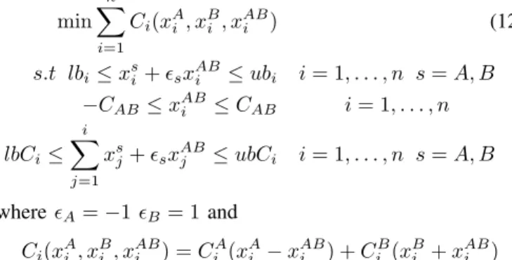
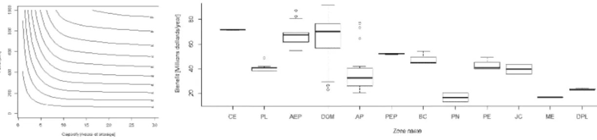
Figure
Documents relatifs
this function has been defined in particular in agreement with [1] which has pointed out that most multimodal functions are not satisfactory for some real-world multimodal
This lets the problem more complicated, as various constraints appeared, related to the container type’s requirements (e.g. refrigerated containers must be allocated to
number of messages sent by malicious nodes during a given period of time and providing each honest node with a very large memory (i.e., proportional to the size of the system)
In a last step, we first establish a corre- spondence result between solutions of the auxiliary BSDE and those of the original one and we then prove existence of a solution of
S’il s’agit de passer de l’orbite ext´ erieure ` a l’orbite int´ erieure, il suffit d’appliquer un d´ ecr´ ement de vitesse ∆v B au point B (i.e. d’utiliser des
نيبعلالا ةلاح نيب صقنلا هجوأ ةفرعمل كلذو اهسرامي يتلا ةيضايرلا ةطشنلأا تابلطتمل اقفو هيلع اونوكي نأ بجي فادهأ نم هوققحي نأ بجي امو ةيلاعلا تايوتسملل
Unfortunately, RBMS with parametric models can still over-fit the misspecified model class with limited data and Bayesian nonparametric models cannot provide any performance
In addition, thanks to the flat extrinsic gm, the fT of the nanowire channel device showed a high linearity over a wide gate bias range although the maximum value
