CAHIER 08-2002
HABIT FORMATION AND THE PERSISTENCE OF MONETARY SHOCKS
Hafedh BOUAKEZ, Emanuela CARDIA and Francisco J. RUGE-MURCIA
CAHIER 08-2002
HABIT FORMATION AND THE PERSISTENCE OF MONETARY SHOCKS
Hafedh BOUAKEZ1, Emanuela CARDIA1 and Francisco J. RUGE-MURCIA1
1
Centre de recherche et développement en économique (C.R.D.E.) / Centre interuniversitaire de recherche en économie quantitative (CIREQ) and Département de sciences économiques, Université de Montréal
May 2002
_______________________
The authors thank Peter Ireland for helpful discussions. Financial support from the Social Sciences and Humanities Research Council and the Fonds pour la formation de chercheurs et l'aide à la recherche is gratefully acknowledged.
RÉSUMÉ
Ce papier étudie les effets persistants des chocs monétaires sur la production. Il existe une littérature empirique assez riche sur cette persistance, mais les modèles d’équilibre général standards avec prix rigides ne réussissent pas à générer les réponses de la production au-delà de la durée des contrats nominaux. Ce papier construit et estime un modèle d’équilibre général avec rigidités de prix, formation d’habitudes et coût d’ajustement de capital. Le modèle est estimé par le maximum de vraisemblance en utilisant les données américaines sur la production, le stock réel de monnaie et le taux d’intérêt nominal. Les résultats économétriques suggèrent que la formation des habitudes et le coût d’ajustement du capital jouent un rôle important dans l’explication des effets de la politique monétaire sur la production. En particulier, l’analyse des réponses aux impulsions indique que le modèle génère de la persistance et des réponses amples de la production aux chocs monétaires.
Mots clés : formation d’habitudes, persistance endogène, politique monétaire
ABSTRACT
This paper studies the persistent effects of monetary shocks on output. Previous empirical literature documents this persistence, but standard general equilibrium models with sticky prices fail to generate output responses beyond the duration of nominal contracts. This paper constructs and estimates a general equilibrium model with price rigidities, habit formation, and costly capital adjustment. The model is estimated via Maximum Likelihood using US data on output, the real money stock, and the nominal interest rate. Econometric results suggest that habit formation and adjustment costs to capital play an important role in explaining the output effects of monetary policy. In particular, impulse response analysis indicates that the model generates persistent, hump-shaped output responses to monetary shocks.
1
Introduction
In a recent paper, Chari, Kehoe, and McGrattan (2000) find that standard dynamic stochas-tic general equilibrium (DSGE) models with sstochas-ticky prices fail to generate persistent output effects to monetary shocks. More precisely, the response of output to a money growth shock does not last beyond the duration of price contracts, even if contracts are staggered. Hence, unless one assumes an implausibly large degree of price rigidity, this type of models cannot replicate the persistent output response obtained using, for example, a benchmark vector autoregression (VAR). Previous empirical literature based on VARs documents a persistent, hump-shaped response of output to a monetary shock with a peak around 4 to 6 quarters after the shock [see Bernanke and Mihov (1998) and Christiano, Eichenbaum and Evans (1999)]. The failure of DGSE models to replicate this feature of the data, is referred to as “the persistence problem.”
This paper studies the effects of monetary policy on output using a DSGE model with sticky prices, habit formation, and adjustment costs to capital. Price rigidity is modeled as in Calvo (1983), where each firm has a constant exogenous probability of changing its price in every period. Habit formation has been employed previously by (among others) Abel (1990), Constantinides (1990), and Campbell and Cochrane (1999) to study the equity premium puzzle, by Carrol, Overland, and Weil (2000) to explain the growth-to-savings causality, and by Fuhrer (2000) to explain the excess smoothness of consumption and inflation inertia. Because habit-forming agents dislike large changes in consumption, the consumption response to shocks is smoother and more persistent than predicted by the Permanent Income Hypothesis (PIH) with time-separable utility. Since consumption is the largest component in GDP, habit formation is a plausible candidate to explain the output persistent and hump-shaped response to monetary policy shocks.
The model is estimated by the method of Maximum Likelihood (ML) using US data on output, the real money stock, and the nominal interest rate. The ML procedure yields plausible estimates of the structural parameters. Impulse response analysis indicates that monetary shocks lead to a persistent and hump-shaped response of output. Up to 95 percent of the initial effect of a monetary shock on output persists beyond the average duration of price contracts. Comparing impulse responses and persistence measures for different values of the habit formation and capital adjustment cost parameters indicates that habit formation, by itself, does not solve the persistence problem. Instead, habit formation interacts nonlinearly with costly capital adjustment to increase the propagation mechanism of the model. When the fit of the estimated DSGE model is compared with that of an unrestricted VAR, the Mean Squared Error (MSE) of the DSGE model is smaller than the
one of the VAR for output and real money balances and only slightly larger for the nominal interest rate. Variance decomposition indicates that money growth explains more than 50 percent of the (conditional) output variability at horizons of less than a year. In the long run, money growth explains only 27.1 percent of the unconditional output variability while 71.4 percent is explained by technology shocks.
Related papers include Bergin and Feenstra (2000), Dotsey and King (2001), and Dib and Phaneuf (2001). Bergin and Feenstra construct a model where the interaction of materials inputs and translog preferences leads to endogenous output persistence. Translog prefer-ences dissuade firms from charging higher prices by making the elasticity of demand facing a given firm depend on the firm’s relative price. Dotsey and King construct a model that incorporates variable capital utilization, and materials input and labor flexibility. Results indicate that these three features are mutually reinforcing and magnify output persistence. Dib and Phaneuf construct a DSGE model with sticky prices and costly adjustment to labor. Their results show that adding adjustment costs to the labor input generates endogenous output persistence to monetary shocks. After our research was completed, we found a closely related and independent paper by Christiano, Eichenbaum, and Evans (2001). These au-thors examine both output and inflation persistence using a limited participation model that incorporates price and wage rigidities, optimizing and non-optimizing price and wage setting, habit formation, adjustment costs in investment, and variable capital utilization. Although the modeling strategy is similar to ours, they obtain empirical estimates by minimizing the distance between the impulse responses in a VAR and the ones predicted by the model, while we estimate the model by Full Information Maximum Likelihood using the Kalman filter. The Kalman filter allows us to deal with poorly measured or unobserved variables (like the stock of capital) and yields the optimal solution to the problem of predicting and updating state-space models. Their results suggest that wage rigidity and variable capital utilization are also important to explain output persistence in response to monetary shocks. Although apparently distinct, the crucial features of these models work through the same channel to increase output persistence. They prevent the rapid change in the real marginal cost after a monetary shock and lead to stronger nominal rigidity.
The reminder of the paper is organized as follows: Section 2 presents the theoretical model; Section 3 describes the estimation procedure, reports empirical results, and discusses the impulse response functions and variance decompositions implied by the estimated model; and Section 4 concludes.
2
The Model
The economy consists of (i) an infinitely-lived representative household, (ii) a representative final good producer, (iii) a continuum of intermediate good producers indexed by i∈ [0, 1] , and (iv) a government. Intermediate goods are used in the production of the final good. The final good is perishable and can be used for either consumption or investment. There is no population growth. The population size is normalized to one.
2.1
Households
The representative household maximizes lifetime utility defined by: Ut= Et
∞
X
s=t
βs−tus(cs, cs−1, ms, `s),
where β ∈ (0, 1) is the subjective discount factor and u(·) is the instantaneous utility func-tion. Households derive utility from the consumption of the final good (ct), real money balances (mt), and leisure (`t). The household’s preferences exhibit internal habit forma-tion. That is, utility depends on current consumption relative to a habit stock determined by the household’s own past consumption. Then, consumption in adjacent periods are complements. In particular, the instantaneous utility function is assumed to be:
ut(ct, ct−1, mt, `t) = (ct/cγt−1)1−η1 1− η1 +bt(mt) 1−η2 1− η2 +ψ(`t) 1−η3 1− η3 , (1)
where mt = Mt/Pt, Mt is the nominal money stock, Pt is the aggregate price index, bt is a preference shock, ψ > 0 measures the weight of leisure in the utility function, and η1, η2, and η3 are positive preference parameters different from one. In the special case where ηj → 1 for j = 1, 2, 3, the logarithmic utility function is obtained. In the special case where γ = 0, there is no habit formation and households care only about the absolute level of current consumption. In principle, the habit stock could also include consumption levels prior to time t− 1. Fuhrer (2000) estimates a model where the stock of habit is a weighted average of past consumption and finds that the habit-formation reference level is essentially the previous period’s consumption level.
In addition to money, households can hold interest-bearing one-period nominal bonds. The gross nominal interest rate on bonds due at time t+1 is denoted by Rt. The household’s resources in period t consist of the principal and the return on bonds purchased at time t−1, money holdings set aside in period t− 1, wages and rents received from selling labor and renting capital to firms, dividends, and lump-sum transfers from the government.
The household’s income in period t is allocated to consumption, investment, money holdings, and the purchase of nominal bonds. Investment increases the household’s stock of capital according to:
kt+1 = (1− δ)kt+ xt, (2)
where δ ∈ (0, 1) is the depreciation rate of capital. The capital stock is costly to adjust. The adjustment-cost function is assumed to be quadratic on investment and strictly convex: Γ(xt, kt) = (χ/2)(xt/kt− δ)2kt, (3) where χ ≥ 0. Investment beyond that required to replace depreciated capital, entails a positive quadratic cost that is proportional to the current capital stock.
The representative household’s budget constraint (expressed in real terms) is:
ct+ at+ mt+ xt ≤ (Rt−1/πt)at−1+ (mt−1/πt) + wtnt+ qtkt+ dt+ τt− (χ/2)(xt/kt− δ)2kt, (4) where at= At/Pt is the real value of nominal bond holdings, Atare nominal bond holdings, πt is the gross rate of inflation between t− 1 and t, wt is the real wage, nt is the number of hours worked, qt is the real rental rate of capital, dt are dividends, and τt are lump-sum transfers or taxes. The household’s total endowment of time is normalized to one. Thus:
`t+ nt= 1. (5)
The representative household maximizes its lifetime utility subject to the constraints (4), (5) and the no-Ponzi-game condition. The first-order necessary conditions associated with the optimal choice of ct, Mt, `t, kt+1, and At for this problem are:
λt = (1/c γ t−1)(ct/c γ t−1)−η1 − βγEt[(ct+1/c 1+γ t )(ct+1/ct)−η1], (6) btm−ηt 2 = λt[(Rt− 1)/Rt], (7) (1− nt)−η3 = λtwt/ψ, (8) λt = βEt{λt+1[1 + qt+1− δ + χ(xt+1/kt+1− δ) + (χ/2)(xt+1/kt+1− δ)2]} 1 + χ(xt+1/kt+1− δ) , (9) λt = βRtEt(λt+1/πt+1) , (10)
where λt is the Lagrange multiplier associated with the household’s budget constraint at time t and equals the marginal utility of consumption at time t. Condition (7) determines money demand by equating the marginal rate of substitution of money and consumption to (Rt− 1)/Rt, where Rt is the gross return of the nominal bond. The interest elasticity of money is equal to −1/η2.1 The preference shock bt has the interpretation of a money
1
demand shock. Condition (8) determines labor supply by equating the marginal rate of substitution between labor and consumption to the real wage. Condition (9) prices (the marginal unit of) capital. Condition (10) prices the nominal bond. Conditions (9) and (10) imply that the ex-ante real interest rate should be equal to the ex-ante real return on capital.
2.2
The Final Good Producer
Final good producers are perfectly competitive and aggregate the intermediate goods into a single perishable commodity. Their technology is constant elasticity of substitution (CES):
yt = ·Z 1 0 yt(i)(θ−1)/θdi ¸θ/(θ−1) , (11)
where y(i) is the input of intermediate good i, and θ > 1 is the elasticity of substitution between different goods. As θ→ ∞, goods become perfect substitutes in production. The final good producer solves the static problem
M ax Ptyt−R01Pt(i)yt(i)di, {yt(i)}
subject to (11). Pt(i) is the price of the intermediate good i and Pt is the aggregate price index. The solution of this problem yields the input demand of good i :
yt(i) = (Pt(i)/Pt)−θyt, (12)
where the elasticity of demand is θ. The zero-profit condition implies that the aggregate price index is given by:
Pt=
·Z 1 0 Pt(i)
(1−θ)di¸1/(1−θ). (13)
2.3
The Intermediate Good Producer
The representative firm i produces its differentiated good using the Cobb-Douglas technology:
yt(i) = ztkt(i)αnt(i)1−α, (14)
where 0 < α < 1 and zt is a serially correlated technology shock. The technology shock is common to all intermediate good producers. Unit-cost minimization determines the demands for labor and capital inputs. Formally,
M in wtnt(i) + qtkt(i), {nt(i), kt(i)}
subject to ztkt(i)αnt(i)1−α = yt(i)≥ 1. First-order conditions are:
wt = (1− α) φt[yt(i)/nt(i)], (15)
and
qt = αφt[yt(i)/kt(i)], (16)
where the real marginal cost (φt) is the Lagrange multiplier associated with the constraint. Since technology is common, and labor and capital are perfectly mobile across industries, conditions (15) and (16) imply that all firms must have the same capital/ labor ratio.
Intermediate-good producers are monopolistically competitive. Each firm faces the down-ward slopping demand curve (12) for its differentiated good. Firm i chooses its (nominal) price P (i) taking as given aggregate demand and the price level. Nominal prices are assumed to be sticky. Price stickiness is modeled `a la Calvo [Calvo (1983)]. That is, a firm changes its price with constant and exogenous probability 1− ϕ in every period. Alternatively, one could assume explicit costs of changing prices or Taylor’s staggered price setting. Esti-mating a model with menu costs would deliver an estimate of theses costs as proportion of GDP, but not an estimate of the average length of price contracts. In the Calvo model, the average duration of price contracts is given by 1/(1− ϕ). Aggregation is somewhat easier using Calvo-type than Taylor-type price rigidity because it is not necessary to keep track of heterogeneous price cohorts. From the point of view of estimating the average length of price contracts, Calvo’s model is also easier to implement because the log likelihood func-tion is continuous on ϕ. This follows from the fact that the probability of prices changes is continuous in the interval [0, 1]. On the other hand, the contract length in Taylor’s model is an integer number and, consequently, the log likelihood function is discontinuous on this parameter.
Let us denote by Pt∗the optimal price set by a typical firm at period t. It is not necessary to index Pt∗ by firm because all the firms that change their prices at a given time, choose the same price [see Woodford (1996)]. The total demand facing this firm at time s for s≥ t is ys(i) = (Pt∗/Ps)−θys. The probability that Pt∗ “survives” at least until period s, for s≥ t, is ϕs−t. Then, the intermediate good producer chooses P∗
t to maximize: Et ∞ X s=t (βϕ)s−tΛt,s(Pt∗ − Φs) ys(i),
where Λt,s= (λs/Ps)/(λt/Pt) and Φs is the nominal marginal cost at time s. Differentiating with respect to Pt∗ yields:
Pt∗ = Ã θ θ− 1 ! Ã EtP∞s=t(βϕ)s−tΛt,sysΦs EtP∞s=t(βϕ)s−tΛt,sys ! . (17)
Equation (17) shows that the optimal price depends on current and expected future demands and nominal marginal costs. Due to price stickiness, the equilibrium markup is not constant, as it would be if prices were flexible.
Assuming that price changes are independent across firms, the law of large numbers implies that 1− ϕ is also the proportion of firms that set a new price each period. The proportion of firms that set a new price at time s and have not changed it as of time t (for s≤ t), is given by the probability that a time-s price is still in effect in period t. It is easy to show that this probability is ϕt−s(1− ϕ). It follows that the aggregate price level can be written as: Pt = Ã (1− ϕ) t X s=−∞ ϕt−st (Pt∗)1−θ ! 1 1−θ . This expression may be written in recursive form as:
Pt1−θ = ϕPt−11−θ+ (1− ϕ) (Pt∗)1−θ. (18)
2.4
The Government
The government comprises both fiscal and monetary authorities. There is no government spending or investment. The government makes lump-sum transfers to households each period. Transfers are financed by printing additional money in each period. Thus, the government budget constraint is:
τt= mt− mt−1/πt, (19)
where the term in the right-hand side is seigniorage revenue at time t. Money is supplied exogenously by the government according to Mt = µtMt−1, where µtis the (stochastic) gross rate of money growth.2 In real terms, this process implies
mtπt= µtmt−1. (20)
2.5
Stochastic Shocks
The economy is subject to shocks to technology (zt), money supply growth (µt), and money demand (bt). These shocks follow the exogenous stochastic processes:
ln zt+1 = (1− ρz) ln z + ρzln zt+ ²z,t, (21) ln µt+1 = (1− ρµ) ln µ + ρµln µt+ ²µ,t, (22)
ln bt+1 =
³
1− ρb´ln b + ρbln bt+ ²b,t, (23)
2It is easy to extend the model to allow an endogenous process for money supply whereby money growth
(or the nominal interest rate) follows, for example, a Taylor-type rule. In this extension of the model, the endogenous reaction of the government might also increase the persistence of monetary shocks.
where ρz, ρµ, and ρb are strictly bounded between
−1 and 1 and the innovations ²t = (²z,t, ²µ,t, ²b,t)0 are assumed normally distributed with zero mean and variance-covariance matrix: V= V ar(²t²0t) = σ2²z 0 0 0 σ2 ²µ 0 0 0 σ2 ²b . (24)
Since households are identical, the net supply of (private) bonds is zero. Goods market clearing requires that aggregate output be equal to aggregate demand:
yt = ct+ xt. (25)
A symmetric equilibrium for this economy is a collection of 13 sequences (ct, mt, nt, xt, kt+1, yt, λt, φt, Pt, Pt∗, qt, wt and Rt)∞t=0 satisfying (i) the accumulation equation (2), (ii) the household’s maximization conditions [eq. (6) to (10)], (iii) the production function [eq. (14)], (iv) the cost minimization conditions [eq. (15) and (16)], (v) the pricing conditions [eq. (17) and (18)], (vi) the market clearing condition [eq. (25)], and (vii) the money supply process (20), given the initial stocks of habit, real balances, and capital, and the exogenous stochastic processes (zt, µt, bt).
Since the model cannot be solved analytically, the equilibrium conditions are log-linearized around the deterministic steady state to obtain a system of linear difference equations. [See Appendix A for the log-linearized version of the model.] After some manipulations, the log-linearized version of the model can be written as:
" Xt+1 EtYt+1 # = " A11 A12 A21 A22 # " Xt Yt # + " B1 B2 # Zt+1, (26) Zt+1 = ρZt+ ²t+1, (27)
where Xt = (ˆkt, mˆt−1, ˆct−1)0 is a 3 × 1 vector that contains the predetermined variables of the system (the circumflex denotes percentage deviations from the deterministic steady state); Yt = (ˆct, ˆπt, ˆλt, ˆqt)0 is a 4× 1 vector that contains the forward looking variables; Zt = (ˆzt, ˆµt, ˆbt)0 is a 3× 1 vector that contains the exogenous shocks; ²t = (²z,t, ²µ,t, ²b,t)0 is a 3× 1 vector with the innovations of zt, µt, and bt, respectively; ρ is a 3× 3 diagonal matrix with elements ρz, ρµ and ρb; and A
11, A12, A21, A22, B1, and B2 are submatrices of appropriate size that contain combinations of structural parameters. The Blanchard-Kahn forward-backward solution method can be applied to (26) to obtain:
Xt+1 = A11Xt+A12Yt+B1Zt, (28)
where F1and F2 are both 4×3 matrices that include nonlinear combinations of the structural parameters contained in A11, A12, A21, A22, B1, and B2. For the precise form of these matrices and the conditions for a unique solution, see Blanchard and Kahn (1980). Finally, the remaining (static) variables of the model can be collected in the 6× 1 vector St = (ˆxt, ˆ
nt, ˆwt, ˆφt, ˆRt, ˆyt)0 that follows
St= CXt+ DZt, (29)
where C and D are matrices of size 6× 3 whose elements are also nonlinear combinations of structural parameters.
3
Econometric Analysis
3.1
Estimation Method and Data
The model is estimated by the method of Maximum Likelihood (ML) using the Kalman filter. Previous papers that use ML procedures to estimate DGSE models include Christiano (1988), Altug (1989), Bencivenga (1992), McGrattan (1994), Hall (1996), McGrattan, Rogerson, and Wright (1997), Kim (2000), and Ireland (2001). The estimation strategy used here is closest to the one used by Ireland (2001). The Kalman filter allows us to deal with unobserved or poorly measured predetermined variables (like the stock of capital) and yields the optimal solution to the problem of predicting and updating state-space models. Hansen and Sargent (1998) show that the ML estimator obtained by applying the Kalman filter to the state-space representation of DGSE models is consistent and asymptotically efficient.
For the Kalman-filter estimation procedure, the transition (or state) equation is con-structed using equations (27) and (28) to collect the predetermined and exogenous variables of the system into the 6× 1 vector Ht = (Xt Zt)0 = (kt, mt−1, ct−1, zt, µt, bt)0 that follows the process: Ht+1= QHt+et+1, (30) where Q= " A11+A12F1 A12F2+B1 0 ρ #
is a 6× 6 matrix and et= (0, 0, 0, ²t)0 = (0, 0, 0, ²zt, ²µt, ²bt, )0 is a 6× 1 vector.
The measurement equation consists of the processes for output, the real money stock, and the nominal interest rate. After some fairly straightforward transformations, these variables are written as functions of Ht :
where ξt = (mt, yt, Rt)0 is a 3× 1 vector and W is a 3 × 6 matrix.3 The elements of Q and W are nonlinear functions of the structural parameters of the model. These elements are computed from the Blanchard-Kahn solution of the DSGE model in each iteration of the optimization procedure. Note that the estimation procedure imposes all restrictions implied by the theoretical model. Standard errors were computed as the square root of the diagonal elements of the inverted Hessian of the (negative) log likelihood function evaluated at the maximum. In order to assess the robustness of the results to deviations from the assumption of normality, robust Quasi-Maximum Likelihood (QML) standard errors [White (1982)] were also computed. At the estimated ML parameters, the condition for existence of a unique model solution is satisfied. That is, the number of explosive characteristic roots of the system of linear difference equations equals to the number of non-predetermined variables.
The model was estimated using quarterly US data on output, real money, and the rate of nominal interest. The series were taken from the database of Federal Reserve Bank of St.-Louis. The sample is 1960:Q1 to 2001:Q2. Output is measured by real GDP per capita. The stock of nominal money is measured by M2 per capita. By measuring these two series in per capita terms, we aim to make the data compatible with our model, where there is no population growth. Population is measured by the civilian, noninstitutional population, 16 years old and over. The gross nominal interest rate is measured by the 3-month US Treasury bill rate. Since the variables in the model are expressed in percentage deviations from the steady state, the output and real money series were logged and detrended linearly. The nominal interest rate series was logged and demeaned. We also estimated the model using HP filtered data with very similar results to the ones reported below.4
3.2
Estimates of Structural Parameters
The structural parameters estimated are the preference parameters η2 and η3, the habit per-sistence parameter (γ), the probability of a price change by an intermediate good producer
3As it is well known, estimating DSGE models using more observable variables than structural shocks
leads to a singular variance-covariance matrix of the residuals. See Ingram, Kocherlakota, and Savin (1994) for a discussion in the special case where the only shock is a technology shock. One strategy to address this issue is to add measurement errors to the observable variables [for example, as in McGrattan (1994)]. A possible drawback of this approach is that measurement error lacks a structural interpretation and essentially captures specification error. Still, in preliminary work, we considered this approach. When we added measurement errors to all observable variables, we found that not all variances were identified or that some of them converged to zero. When we added only as many errors as needed to make the system nonsingular, we found that results were very sensitive to the variable that was assumed to be measured with noise.
(ϕ), the parameter of the cost of capital adjustment function (χ), and parameters of the shock processes (ρz, ρµ, ρb, σz, σµ and σb). Remaining parameters were either poorly identified or additional evidence about their magnitude is available. Data on national income accounts suggest that a plausible value for the share of capital in production is 0.36. The subjective discount factor is fixed to 0.99, meaning that the steady state gross real interest rate is ap-proximately 1.01. The rate of depreciation is fixed to 0.025. The gross rate of money growth (and inflation) at the steady state is fixed to 1.017. This value corresponds to the average gross rate of money growth during the sample period. Two important structural parame-ters that are poorly identified are the curvature parameter of the consumption component in the utility function (η1) and the elasticity of demand (θ). Markup estimates reported by Basu and Fernald (1994) for US data indicate that θ is approximately 10. Estimates of the curvature of the utility function with respect to consumption range from 0.5 to 5. We assume η1 = 2, but sensitivity analysis indicates that the results do not depend crucially on the magnitudes of θ and η1.5 Finally, fixing the proportion of time worked in steady date (n) amounts to fixing either the mean of the technology shock (z) or the weight of leisure in the utility function (ψ). We do not assign particular values to these parameters during the estimation procedure. Instead, we adjust them so that along with the ML estimate of η3, n = 0.31. This means that the proportion of time worked in steady state is approximately one third.
ML estimates of the parameters and their asymptotic and QML standard errors are re-ported in Table 1. Since asymptotic and QML standard errors have very similar magnitudes, conclusions regarding the statistical significance of the parameters do not depend on the es-timate of the standard error employed to construct the t-statistic. The ML eses-timate of the habit-formation parameter (γ) is 0.98 (0.016). The term is parenthesis is the asymptotic standard error of the estimate. This estimate is significantly different from zero, but is not significantly different from one, at standard levels. This estimate is larger than, but still consistent with, the values of 0.80 (0.19) and 0.90 (1.83) reported by Fuhrer (2000), 0.63 (0.14) reported by Christiano, Eichenbaum and Evans (2001), 0.73 reported by Boldrin, Christiano and Fisher (2001), and 0.938 (1.775) reported by Heaton (1995).
The estimated value of the adjustment-cost parameter (χ) is 85.19 (18.94). In order to give meaning to this estimate and to allow its comparison with estimates based on other functional forms, it is useful to compute the elasticity of investment with respect to the price of installed capital. The elasticity implied by the estimate of χ is 0.47. This value
5We also performed single and joint Lagrange Multiplier tests of the null hypothesis that the true values of
β, δ, η1, α, and θ are the ones assumed during estimation. In all cases, one cannot reject the null hypothesis.
is higher than the point estimates of 0.34 and 0.28 reported by Kim (2000) and Christiano, Eichenbaum, and Evans (2001), respectively, but it is considerably lower than the typical value used to calibrate standard Real Business Cycle (RBC) models [see, for example, Baxter and Crucini (1993)].
The estimated probability of not changing price in a given quarter or, equivalently, the proportion of firms that do not change prices in a given quarter is 0.847 (0.034). This implies that the average length of price contracts is 1/(1− 0.847) = 6.56 (1.44) quarters. Previous estimates on the average time between price adjustments vary substantially. Gal´i and Gertler (1999) find that θ is approximately 0.83. Their estimate implies that prices are fixed between five and six quarters. Cechetti (1986) reports that the average number of years since the last price adjustment for US magazines ranges from 1.8 to 14. Kashyap (1995) finds that the average time between price changes in 12 mail-order catalog goods is approximately 4.9 quarters. Taylor (1999) surveys empirical studies on price setting and finds that the average duration of price contracts is about 4 quarters in the United States. Bils and Klenow (2001) document substantial heterogeneity in the frequency of price adjustments among the goods surveyed by the US Bureau of Labor Statistics and report a median price duration of only 1.66 quarters. Christiano, Eichenbaum, and Evans (2001) find that the average length of price contracts is about 2 quarters and that of wage contracts is roughly 3.3 quarters.
The parameter estimates imply that the interest elasticity of money is 0.32 and the consumption elasticity of money of 0.65. The former estimate is very close to the one of 0.39 reported by Chari, Kehoe and McGrattan (2000), but larger than the ones found by Christiano, Eichenbaum, and Evans (2001) and Dib and Phaneuf (2001) of 0.10 and 0.11 respectively.
From the estimate of the curvature parameter of the leisure component in the utility function (η3), we can compute an estimate of the elasticity of labor supply with respect to the real wage (for a given marginal utility of consumption) as (1− n)/(η3n) = (1 − 0.31)/(1.591· 0.31) = 1.4 (2.99). See Appendix A. However, this estimate is too imprecise to allow reliable conclusions.
Finally, estimates of the autoregressive coefficients of the shock processes indicate that all shocks are very persistent. Very persistent technology and money demand shocks are also reported by Kim (2000), Ireland (2001) and Dib and Phaneuf (2001). The estimate of ρµ is higher than values found when money growth is estimated using an univariate process [for example, as in Chari, Kehoe, and McGrattan (2000)].
3.3
Fit and Specification Tests
This section evaluates the goodness of fit of the model, compares it with that of an unre-stricted VAR, and performs specification tests on the model residuals. Figure 1 plots the observed and fitted series of US real money balances, output, and the nominal interest rate. This Figure indicates that the model tracks very well the dynamics of these variables. A standard measure of goodness of fit is the R2, that measures the proportion of the total variation in the dependent variable that is explained by the model. The R2s for real money balances, output, and the nominal interest rate are 0.945, 0.948, and 0.893, respectively. Thus, roughly 95 percent of the total variation of the real money stock and output can be explained by the DSGE model with sticky prices, habit formation, and costly capital adjust-ment. The model does not explain as well the behavior of the nominal interest rate, but still can account for more than 89 percent of the total variation of this series.
It is instructive to compare the fit of the model with the one of an unrestricted VAR. The VAR is of order one and contains the following US variables: real money stock, output, and the nominal interest rate. The comparison is made in terms of the Mean Squared Error (MSE).6 The MSE is defined as:
M SE = Ã T X t=2 (Xt− ˆXt)2 ! /(T − 1),
where T = 166 is the number of observations, Xt is either output, real money balances, or the rate of nominal interest, and ˆXt is the value predicted by the model. Since the VAR uses the first observation in the sample to construct the lag, the number of observations used to construct the MSE is T − 1 = 165. Table 2 reports the MSE from the estimated DSGE model and the VAR. The DSGE model outperforms the VAR when explaining the behavior of US output and real money balances in the sense that its MSE is smaller. However, for the nominal interest rate, the MSE of the VAR is slightly less than the one of the DSGE model.
Table 3 reports test results for serial correlation of the residuals (Panel A) and neglected Autoregressive Conditional Heteroskedasticity (ARCH) (Panel B). Consider first the Durbin-Watson test for first-order autocorrelation. Comparing the test statistic with the 5 percent critical value of its tabulated distribution indicates that (i) one cannot reject the null hy-pothesis of no autocorrelation for the real money balances and output residuals, but (ii) one can reject it for the nominal interest rate residuals. Similarly, results of Pormanteau tests
6Note that the state-space and VAR models are nonnested, and, consequently, standard Likelihood Ratio,
for first- to third-order autocorrelation of the residuals yield statistics that are below (above) their 5 percent critical value for real money balances and output (nominal interest rate).7
The Lagrange Multiplier (LM) tests for neglected ARCH were computed as the product of the number of observations and the uncentered R2 of the OLS regression of the squared residual on a constant and one to three of its lags. Under the null hypothesis of no conditional heteroskedasticity, the statistic is distributed chi-square with as many degrees of freedom as the number of lagged squared residuals included in the regression. Results in Panel B indicate that the null of hypothesis of no conditional heteroskedasticity cannot be rejected at the 5 percent level for output and real money balances, but that it can be rejected for the nominal interest rate in some cases. All these results indicate that the model tracks well the behavior of US output and real money balances but is somewhat less successful explaining the nominal interest rate.
The model also generates predictions regarding series whose actual data were not used in the estimation procedure. For example, consumption, investment, the rate of inflation, and the real marginal cost. The real marginal cost is not directly observable, but under certain conditions, it can be proxied by the labor share in national income [see Gal´i and Gertler (1999) for a detailed discussion]. Figure 2 plots the observed and predicted series of US consumption, investment, inflation, and the real marginal cost. From this Figure, it is clear that the model generates consumption and investment dynamics that are similar to the ones of their detrended US counterparts. However, predicted investment is much smoother than the data.
The model does a poor job explaining the behavior of the real marginal cost and inflation. This result reflects a drawback of inflation models based on forward-looking pricing rules. It is possible to show that under Calvo-type pricing, the inflation deviation from steady state equals the present discounted value of current and future expected real marginal cost deviations from steady state.8 This means that inflation inherits the dynamic properties of the real marginal cost and that current inflation is not helpful in predicting future inflation. Because lagged inflation is absent from the inflation equation, forward-looking pricing rules imply that inflation is less persistent than usually found in the data. To address this shortcoming of the model, some authors [for example, Gal´i and Gertler (1999)] assume the existence of rule-of-thumb firms that fix their prices as a function of past inflation. Another problem with our model is that the real marginal cost is more volatile than the labor share
7Under the null hypothesis of no autocorrelation, the Portmanteau test statistic is distributed chi-square
with as many degrees of freedom as autocorrelations are tested for.
8This result can be easily derived by rewriting equation (A1) in Appendix A with current inflation in the
in national income would suggest. One possibility is that the labor share in national income is a poor empirical proxy for the real marginal cost. More likely, the real marginal cost in our model is excessively volatile because it abstracts from supply-side features like variable capital utilization and adjustment costs to labor input.
3.4
Impulse-Response Analysis
This section examines the response of the economy to a shock to the growth rate of the money supply. Hereafter, we refer to this shock as a money supply shock. The intention here is (i) to assess the ability of the model to match the persistent output effect of monetary policy shocks documented in the VAR literature, and (ii) to investigate the role of habit formation and costly capital adjustment in solving the persistence problem. We compare the impulse response functions calculated using the estimated parameters with those obtained using two polar, counterfactual versions of the model. The first version assumes adjustment costs of capital but no habit formation. The second version assumes habit formation but no adjustment costs of capital.
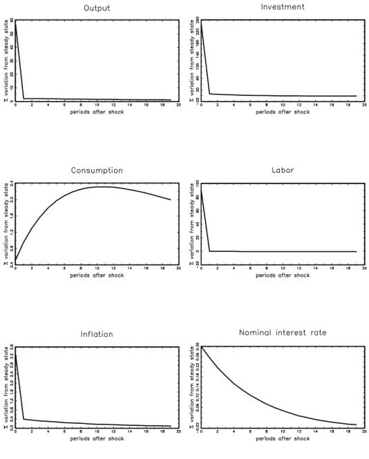
Figure 3 plots the impulse responses of output, investment, consumption, labor, inflation, and the nominal interest rate to a 1 percent money supply shock. Following the shock, there is an increase in aggregate demand that causes output and consumption to increase. The consumption response is hump-shaped because under habit formation, agents smooth both the level and the change of consumption. The output response is also hump-shaped as in previous VAR literature. The peak of the output (consumption) response takes place after two (four) quarters, rather than the four to six quarters usually found in VAR models.
Since the effect of the money supply shock on output dies out very slowly, the dynamic path of output is persistent. As a measure of the endogenous persistence of output generated by the model, we compute the proportion of the impact effect that persists beyond the average length of price contracts. Recall that the estimated probability of price changes implies an average duration of price contracts of 6.56 quarters. Thus, the measure of endogenous persistence is:
ζ ≡ κ(7)/κ(0),
where κ(j) is the impulse response coefficient at lag j. In this case, ζ = 0.95, meaning that 95 percent of the initial effect of the monetary shock on output persists beyond seven quar-ters. This indicates that the estimated model produces a substantial amount of endogenous persistence.
Figure 3 also shows that investment and labor increase following a (positive) monetary shock. This result is due to the fact that aggregate demand is expected to increase in
subsequent periods because prices adjust slowly. The nominal interest rate also rises after a positive monetary shock. Thus, the model does not generate a liquidity effect. A more detailed explanation of this results is presented below.
Figure 4 plots the impulse responses generated from a model with price stickiness, adjust-ment costs to capital but no habit formation. The parameter γ is set to zero and remaining parameters are set to their ML estimates. In contrast to the previous model, output and consumption responses are not hump-shaped. Both variables jump immediately after the monetary shock and return gradually to their steady state levels. The output response is less persistent than the one in Figure 3. Since ζ = 0.30, this version of the model with no habit formation delivers only 30 percent of endogenous persistence. This suggests that habit formation might be an important ingredient in explaining the persistence of output in response to monetary shocks.
Figure 5 shows the impulse responses corresponding to a model with price stickiness, habit formation but no adjustment costs to capital. The parameter χ is set to zero and remaining parameters are set to their ML estimates. A positive monetary shock triggers a large initial increase in output, investment, hours worked, and inflation, but the variables drop sharply in the following period and return close to their steady state levels. In order to understand the output response, note that investment must increase to accommodate the upward shift in future demand. However, since capital is free to adjust, all the required increase in investment takes place immediately after the shock. This version of the model does not generate any significant amount of endogenous persistence: ζ = 0.03 meaning that only 3 percent of the initial effect of the monetary shock persists after seven quarters. Kim (2000) and Dib and Phaneuf (2001) report a similar dynamic path of output using models with price stickiness only. This suggests that habit formation alone does not solve the persistence problem. Instead, habit formation plays the role of a catalyst that, combined with additional features, helps to spread out the effects of monetary shocks. In this model, the additional feature is the adjustment costs of capital.
The increase in the nominal interest rate following a monetary shock is larger in Figure 4 than in Figure 5. This result is consistent with Kim’s (2000) finding that real rigidities help to generate a liquidity effect in DSGE models. However, as seen in Figure 3, adjustment costs to the capital stock are not enough to generate a liquidity effect in this model. The reason is that the estimated money growth process is highly autocorrelated. Thus, after a positive money supply shock, expected inflation increases by a magnitude that is larger in absolute value than the decrease in the real interest rate. As a result, the net effect of the money shock on the nominal interest rate is positive.
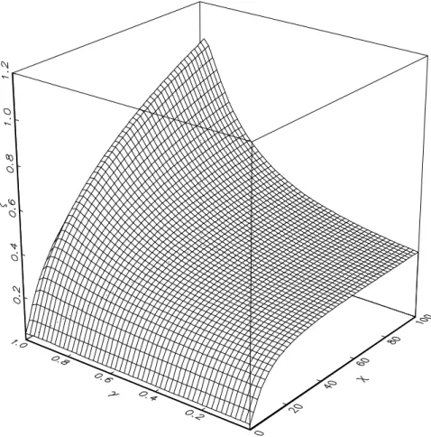
adjust-ment costs to capital might be important features in a model that seeks to explain the persistent output response to monetary policy shocks. In order to further understand the relationship between endogenous output persistence and the parameters that control habit formation and capital adjustment costs, the persistence measure, ζ, is computed for different combinations of the parameters γ and χ. The resulting three-dimensional graph is plotted in Figure 6. In this Figure, γ varies from 0 to 1, and χ varies between 0 and 100. The Figure shows that habit formation increases the output persistence of monetary shocks only to the extent that capital adjustment costs are not in the neighborhood of zero. The in-crease in persistence is bounded at fairly low levels unless γ is sufficiently large. Hence, habit formation and adjustment costs of capital interact in a non-linear way to increase the output persistence of monetary policy shocks. This finding parallels the one in Bergin and Feenstra (2000), where the nonlinear interaction of materials inputs and translog preferences increases endogenous output persistence.
Although we are primarily concerned with the effects of monetary policy shocks, the estimated model generates predictions regarding the effect of technology and money demand shocks. The response of output, investment, consumption, hours worked, inflation, and the nominal interest rate to a 1 percent technology shock is plotted in Figure 7. Because prices are rigid, the aggregate supply curve is upward sloping. A positive technology shock shifts the aggregate supply curve to the right. Consequently, output increases and prices decrease. The response of output and consumption is persistent and hump-shaped. Hours worked decrease in a persistent manner following a technology shocks. The intuition of this result is as follows. After a positive technology shock, the firm will be able to satisfy current demand with a lower level of inputs, so labor input will decrease on impact. Eventually, as demand increases and capital is adjusted, labor demand increases. A similar decline of labor in response to a technology shock is reported by Gal´i (1999) using a structural vector autoregression, and by Dib and Phaneuf (2001) and Vigfusson (2002) using DSGE models.
Finally, the impulse response functions generated by a 1 percent money demand shock are plotted in Figure 8. Since money supply is unchanged and prices are rigid, this shock produces a downward shift of aggregate demand in current and subsequent periods. Conse-quently, output, consumption, hours worked, and investment decrease. As a result of habit formation, the response of consumption has an inverted hump shape with a trough around three periods after the shock.
3.5
Variance Decomposition
In this section, we study the relative importance of monetary shocks for the fluctuations of output, investment, consumption, hours worked, inflation, and the nominal interest rate. To that effect, we compute the fraction of the conditional variance of the forecasts at different horizons that is attributed to each of the model’s shocks. This variance decomposition is plotted in Figure 9. As the horizon increases, the conditional variance of the forecast error of a given variable converges the unconditional variance of that variable. The decompositions of the unconditional variances are reported in Table 4. Recall that a money supply shock is a shock to the growth rate of the money supply while the money demand shock is a shock to the preference parameter of money in the utility function. Several results are apparent from Figure 9 and Table 4. First, money demand shocks play an important role in explaining the fluctuations of the nominal interest rate. At horizons of less than six quarters, money demand shocks explain more than 50 percent of the conditional variance of the nominal interest rate. In the long-run, money demand shocks explain roughly 45 percent of the conditional variance of the nominal interest rate. Second, money supply shocks explain most of the fluctuations of the rate of inflation at all horizons. Third, technology shocks explain most of the variation in hours worked at all horizons. Fourth, money supply shocks account for the largest part of the conditional variance in forecasting investment in the short-run. As the horizon increases, the contribution of technology shocks increases and the one of money supply shocks decreases but even in the long-run, money supply shocks explain half of the variance of investment. Fifth, money supply shocks and technology shocks are equally important in explaining the conditional variance of consumption in the very short run. However, as the horizon increases the contribution of technology shocks increases and that of money supply shocks decreases. In the long-run, 77.3 percent of the variance of consumption is explained by technology shocks and only 21.6 percent by money supply shocks. Finally, money supply shocks account for the largest part of the conditional variance in forecasting output in the short run (i.e., less than a year). At higher horizons, most of the conditional variance is due to technology shocks. In the long-run, 27 percent of the unconditional variance of output is attributed to money supply shocks, 2 percent to money demand shocks, and 71 percent to technology shocks.
4
Conclusion
This paper constructs a DSGE model with sticky prices, habit formation, and costly capital adjustment that accounts for the persistent and hump-shaped response of output to monetary
shocks. Although habit formation, by itself, does not solve the persistence problem, it interacts nonlinearly with costly capital adjustment to increase the internal propagation mechanism of the model.
The model is estimated by the method of Maximum Likelihood (ML) using US data on output, the real money stock, and the nominal interest rate. Econometric results indicate that US prices are fixed on average for six and a half quarters. Although the peak of the output response takes place after two quarters, that is less than the four to six quarters usually found in VAR models, up to 95 percent of the initial effect of a monetary shock on output persists beyond the average duration of price contracts. Variance decomposition indicates that money growth explains more than 50 percent of the (conditional) output variability at horizons of less than a year. In the long run, money growth explains only 27.1 percent of the unconditional output variability while 71.4 percent is explained by technology shocks.
The DSGE fits US output and real money balances better than an unrestricted VAR and does only slightly worse for the nominal interest rate. The model also tracks well the behavior of consumption and investment, but it does a poor job explaining the US inflation rate. This is partly the result of the forward-looking pricing rule and the prediction that the real marginal costs is much more volatile than the data. Including additional features would allow DSGE models to capture other features of the data like inflation persistence and, perhaps, the liquidity effect. In future work, we intent to extend this model to allow for a backward looking component in the price rule that arises directly from first principles.
A
Appendix A : The Log-linearized Model
In what follows, variables without time subscript denote steady state values and the circum-flex denotes percentage deviation from steady state. For example, ˆxt = (xt− x)/x is the percentage deviation of investment from its steady state at time t. Linearizing (2) and the first order conditions (6)-(10) yields:
ˆ kt+1 = (1− δ)ˆkt+ δ ˆxt, Etˆct+1 = à βγ (γ (1− η1) + 1)− η1 βγ (1− η1) ! ˆ ct− à 1 β ! ˆ ct−1+ à βγ− 1 βγ (1− η1) ! ˆ λt, ˆ Rt = η2 à π− β β ! (ˆπt− ˆmt−1− ˆµt)− à π− β β ! ˆ λt+ à π− β β ! ˆbt, ˆ nt = à 1− n nη3 ! ˆ λt+ à 1− n nη3 ! ˆ wt, Etqˆt+1 = à 1 βq ! (ˆλt− Etˆλt+1) + à χ(1 + βδ) βq ! ˆ kt+1− à χ βq ! ˆ kt− à χδ q ! ˆ xt+1, Etλˆt+1 = ˆλt+ Etπˆt+1− ˆRt.
The production function (14) and first order conditions for cost minimization by the inter-mediate good producer (eq. (15) and (16)) become:
ˆ yt = αˆkt+ (1− α) ˆnt+ ˆzt, ˆ wt = φˆt+ ˆyt− ˆnt, ˆ φt = ˆqt− ˆyt+ ˆkt.
The linearized versions of equations (17) and (18) together imply: Etˆπt+1 = 1 βπˆt− Ã (1− ϕ) (1 − ϕβ) ϕβ ! ˆ φt. (A1)
Linearizing the equation defining money growth (20) and the market clearing condition (25) yields: ˆ mt = mˆt−1− ˆπt+ ˆµt, ˆ xt = µ y δk ¶ ˆ yt− µ c δk ¶ ˆ ct.
Finally, the stochastic processes of the shocks (eq. (21)-(23)) are linearized as: ˆ
zt+1 = ρzzˆt+ ²z,t, ˆ
µt+1 = ρµµˆt+ ²µ,t, ˆbt+1 = ρbˆbt+ ²b,t.
Table 1. Maximum Likelihood Estimates
Asymptotic Robust
Description Parameter Estimate S.E. S.E.
Habit-formation parameter γ 0.982 0.016 0.021
Probability of no price change ϕ 0.847 0.037 0.023
Adjustment cost χ 85.188 20.728 29.402
Preference parameter η2 3.089 0.827 1.462
Preference parameter η3 1.591 3.530 3.732
AR coefficient of technology shock ρz 0.867 0.055 0.055
AR coefficient of money supply shock ρµ 0.879 0.035 0.053
AR coefficient of money demand shock ρb 0.924 0.019 0.029
S.D. of technology shock σ²z 0.040 0.027 0.032
S.D. of money supply shock σ²µ 0.007 0.002 0.003
S.D. of money demand shock σ²b 0.077 0.005 0.008
Notes: S.D. and S.E. are standard deviation and standard error, respectively. The restrictions imposed on the parameters were γ, ϕ∈ (0, 1), ρz, ρµ, ρb
∈ (−1, 1), and η2, η3, χ, σ²z, σ²µ, σ²b ∈
Table 2. Goodness of Fit MSE (× 10−5)
Variable DSGE Model Unrestricted VAR(1)
Output 6.073 6.562
Real money stock 4.599 7.841
Nominal interest rate 0.416 0.381
Table 3. Test for Serial Correlation and Neglected ARCH
Real Money Nominal
Output Stock Interest Rate
Panel A. Test for Serial Correlation
Durbin-Watson 2.15 1.98 1.50
Portmanteau
One autocorrelation 1.11 0.002 9.38∗
Up to two autocorrelations 1.11 1.86 14.27∗
Up to three autocorrelations 2.21 4.18 17.32∗
Panel B. LM Test for Neglected ARCH Number of squared lags
One 0.90 3.62 1.82
Two 1.48 3.63 26.77∗
Three 1.63 3.74 28.88∗
Notes: The superscript ∗ denotes the rejection of the null hypothesis that the parameter is zero at the 5 percent significance level.
Table 4. Unconditional Variance Decomposition
Fraction of the Unconditional Variance Due to Technology Money Supply Money Demand
Variable Shocks Shocks Shocks
Output 0.714 0.271 0.015
Investment 0.469 0.493 0.038
Consumption 0.773 0.216 0.011
Labor 0.872 0.120 0.008
Inflation rate 0.221 0.756 0.023
Nominal interest rate 0.163 0.389 0.448
Notes: The money supply shock is a shock to the growth rate of the money supply. The money demand shock is a shock to the preference parameter of money in the utility function.
References
[1] Abel, A. B. (1990), “Asset Prices under Habit Formation and Catching up with the Joneses,” American Economic Review 80, 38-42.
[2] Altug, S. (1989), “Time-to-Build and Aggregate Fluctuations: Some New Evidence,” International Economic Review 30, 889-920.
[3] Basu, S and Fernald, J. (1994), “Constant Returns and Small Markups in US Manufac-turing,” International Finance Discussion Paper 483.
[4] Baxter, M. and Crucini, M. J. (1993), “Explaining Saving-Investment Correlations,” American Economic Review 83, 416-436.
[5] Bencivenga, V. R. (1992), “An Econometric Study of Hours and Output Variation with Preference Shocks,” International Economic Review 33, 449-471.
[6] Bergin, P. and Feenstra, R. (2000), “Staggered Price Setting, Translog Preferences and Endogenous Persistence,” Journal of Monetary Economics 45, 657-680.
[7] Bernanke, B. and Mihov, I. (1998), “Measuring Monetary Policy Shocks,” Quarterly Journal of Economics 113, 869-902.
[8] Bils, M. and Klenow, P. J. (2001), “Some Evidence on the Importance of Sticky Prices,” University of Rochester, Mimeo.
[9] Blanchard, O. J. and Khan, C. M. (1980), “The Solution of Linear Difference Models Under Rational Expectations,” Econometrica 48, 1305-1311.
[10] Boldrin, M., Christiano, L. J., and Fisher, J. (2001), “Habit Persistence, Asset Returns and the Business Cycle,” American Economic Review 86, 1154-1174.
[11] Campbell, J. Y. and Cochrane, J. H. (1999), “By Force of Habit: A Consumption-Based Explanation of Aggregate Stock Market Behavior,” Journal of Political Economy 107, 205-251.
[12] Calvo, G. (1983), “Staggered Prices in a Utility Maximization Framework,” Journal of Monetary Economics 12, 983-998.
[13] Carrol, C. D., Overland, J., and Weil, D. N. (2000), “Saving and Growth with Habit Formation,” American Economic Review 90, 341-355.
[14] Cechetti, S. G. (1986), “The Frequency of Price Adjustment: A Study of the Newsstand Prices of Magazines,” Journal of Econometrics 31, 255-274.
[15] Chari, V., Kehoe, P., and McGrattan, E. (2000), “Sticky Price Models of the Business Cycle: Can the Contract Multiplier Solve the Persistence Problem,” Econometrica, 68, 1151-1179.
[16] Christiano, L. J. (1988), “Why Does Inventory Investment Fluctuate So Much?” Jour-nal of Monetary Economics 21, 247-280.
[17] Christiano, L. J., Eichenbaum, M., and Evans, C. L. (1999), “Monetary Shocks: What Have We Learned and to What End ?,” in J. B. Taylor and M. Woodford, eds., Handbook of Macroeconomics, Amsterdam: North-Holland.
[18] Christiano, L. J., Eichenbaum, M., and Evans, C. L. (2001), “Nominal Rigidities and the Dynamic Effects of a shock to Monetary Policy,” NBER Working Paper 8403. [19] Constantinides, G. M. (1990), “Habit Formation: A Resolution of the Equity Premium
Puzzle,” Journal of Political Economy 98, 519-543.
[20] Dib, A. and Phaneuf, L. (2001), “An Econometric U.S. Business Cycle Model with Nominal and Real Rigidities,” Universit´e du Qu´ebec `a Montr´eal, Working Paper 137. [21] Dotsey, M. and King, R. G. (2001), “Pricing, Production and Persistence,” NBER
Working Paper 8407.
[22] Gal´i, J. (1999), “Technology, Employment and the Business Cycle: Do Technology Shocks Explain Aggregate Fluctuations ?,” American Economic Review 89, 249-271. [23] Gal´i, J. and Gertler, M. (1999), “Inflation Dynamics: A Structural Econometric
Anal-ysis,” Journal of Monetary Economics 44, 195-222.
[24] Fuhrer, J. (2000), “Habit Formation in Consumption and Its Implications for Monetary-Policy Models,” American Economic Review 90, 367-390.
[25] Heaton, J. (1995), “An Empirical Investigation of Asset Pricing with Temporally De-pendent Preference Specifications,” Econometrica 63, 681-717.
[26] Hall, G. J. (1996), “Overtime, Effort, and the Propagation of Business Cycle Shocks,” Journal of Monetary Economics 38, 139-160.
[27] Hansen, L. P. and Sargent, T. J. (1998), “Recursive Linear Models of Dynamic Economies,” University of Chicago, Mimeo.
[28] Ingram, B. F., Kocherlakota, N., and Savin, N. E. (1994), “Explaining Business Cycles: A Multiple-Shock Approach,” Journal of Monetary Economics 34, 415-428.
[29] Ireland, P. (2001), “Sticky Price Models of the Business Cycle: Specification and Sta-bility,” Journal of Monetary Economics 47, 3-18.
[30] Kashyap, A. K. (1995), “Sticky Prices: New Evidence from Retail Catalogs,” Quarterly Journal of Economics 110, 245-274.
[31] Kim, J. (2000), “Constructing and Estimating a Realistic Optimizing Model of Mone-tary Policy,” Journal of MoneMone-tary Economics 45, 329-359.
[32] McGrattan, E. R. (1994), “The Macroeconomic Effects of Distortionary Taxation,” Journal of Monetary Economics 33, 573-601.
[33] McGrattan, E. R., Rogerson, R., and Wright, R. (1997), “An Equilibrium Model of the Business Cycle with Household Production and Fiscal Policy,” International Economic Review 38, 267-290.
[34] Taylor, J. B. (1999), “Staggered Prices and Wage Setting in Macroeconomics,” in J. B. Taylor and M. Woodford, eds., Handbook of Macroeconomics, Amsterdam: North-Holland.
[35] Vigfusson, R. (2002), “Why Does Employment Fall After a Positive Technology Shock: A Neoclassical Explanation,” Northwestern University, Mimeo.
[36] White, H. (1982), “Maximum Likelihood Estimation of Misspecified Models,” Econo-metrica, 50: 1-25.
[37] Woodford, M. (1996), “Control of the Public Debt: A Requirement for Price Stability,” NBER Working Paper 5684.


![[PPT] Cours Langage HTML & XHTML methodes et explications | Cours informatique](data:image/gif;base64,R0lGODlhAQABAIAAAP///wAAACH5BAEAAAAALAAAAAABAAEAAAICRAEAOw==)