Charlot: Université de Cergy-Pontoise, THEMA, F-95000 Cergy-Pontoise, and CIRPÉE ocharlot@u-cergy.fr
Malherbet: Université de Rouen, CARE-EMR, CECO – École Polytechnique, fRDB and IZA
Terra: Université de Cergy-Pontoise, THEMA; Graduate School of Economics, Fundação Getulio Vargas; and CEPII We thank Pedro Miguel Olea de Souza e Silva for excellent research assistance. We also thank participants from PET’10 Conference and from seminars at Université de Cergy-Pontoise, Université du Maine and CEPII for comments and suggestions. The usual disclaimer applies.
Cahier de recherche/Working Paper 10-43
Product Market Regulation, Firm Size, Unemployment and Informality
in Developing Economies
Olivier Charlot
Franck Malherbet
Cristina Terra
Abstract:
This paper studies the impact of product and labor market regulations on the number
and size of firms in the formal and informal sectors, as well as on relative wages, relative
size of the two sectors and overall unemployment. We show that entry costs in the
formal sector tend to make informal firms smaller and more numerous than informal
firms, i.e., such costs render the informal sector relatively more competitive.
Furthermore, it is possible to reduce informality without increasing unemployment or
reducing workers’ wage by reducing entry costs in the formal sector rather than reducing
labor market regulations. We also highlight a number of externalities stemming from
labor and product market imperfections, allowing the size of those distortions to differ
across sectors. We show that, while the so-called overhiring externality takes place in
both sectors, this translates into a smaller relative size of the informal sector.
Keywords: Informality, product and labor market imperfections, firm size
1
Introduction
Informal activities are pervasive in both developed and developing economies. According to Schneider and Enste (2000) estimates, the size of the shadow economy as a percentage of GDP ranges from 25 to 60% in Latin America, from 13 to 50% in Asia, and it is around 15% among OECD countries, reaching 30% in some European countries. Informal firms differ from formal ones in a number of measurable characteristics, and there is a growing literature trying to understand the causes of informality and its differences from formal businesses. Product and labor market regulation are the usual suspects, since they affect the cost of complying to taxes and regulations for a formal firm.
On average, informal firms tend to invest less, to be less productive, to pay lower wages and to hire less skilled workers. Moreover, firms in the informal sector are generally smaller and more
numerous compared to those in the formal sector.1As a result they are prone to enjoy less market
power in the product market. All in all, the informal sector is likely to be more competitive than the formal one. As a matter of fact, the informal sector is usually modeled in the literature as a perfectly competitive one, while firms are assumed to enjoy market power in the formal sector. An important question not yet explored in the literature is precisely what affects the relative degree of competition in the two sectors, and its impact on firms’ behavior in the labor market. This paper studies the impact of product and labor market regulations (hereafter PMR and LMR, respectively) on the number and size of firms in the formal and informal sectors, as well as on relative wages, relative size of the two sectors and overall unemployment.
We build a model with two sectors, a formal and an informal one, where both sectors are subject to imperfect competition in the product market and matching frictions in the labor mar-ket. The two sectors face the same externalities, but are allowed to differ with respect to some parameter values, such as entry costs, taxes paid, the bargaining power of their workers, pro-ductivity, among others. Firm size, labor demand, wages, prices, unemployment and informality size are endogenously determined. In particular, in our model economy firms in the informal sector turn out to be indeed smaller and more numerous than their formal counterparts. As a result, the formal sector is relatively less competitive. We then study the effects of changes in PMR modeled as changes in entry costs in the formal sector, and of changes in LMR, proxied by changes in workers’ bargaining power, on the main endogenous variables of the model. We highlight some externalities related to product and labor market imperfections and study how they affect unemployment and the division of employment between the two sectors.
We simulate the model so as to replicate some of the key characteristics of the Brazilian
economy. We chose Brazil as our benchmark case because it is a developing economy with a large informal sector. Brazil’s informal sector employs around 40% of its labor force, while the country’s unemployment rate ranged from 7% to 13% over the last decade. Moreover, Brazil has relatively high barriers to entry in the product market (Djankov et al., 2002), while labor legislations appear relatively moderate compared to some other Latin American countries (Botero et al., 2004). In this perspective, it is interesting to examine how unemployment and informality would react, had the government chosen a different mix between product and labor market regulations, that is, lower barriers to entry and/or stricter labor regulations.
There is a recent and growing literature on unemployment and informality in developing countries. Our analysis highlights distortions that had not yet been contemplated by previous models as being shared by both formal and informal sectors. In sum, in our model: (i) there are frictions in both formal and informal labor markets; (ii) job seekers are identical and can find jobs in both sectors, that is, the labor market is not segmented; (iii) the number and size of firms in each sector is endogenous, which renders market power also endogenous; (iv) wages are set through bargaining betweenlarge firms and their workers, which generates externalities in the two sectors.
It is worth highlighting that, with respect to the labor market, we consider two sources of distortions. First, there are the standard congestion externalities linked to the matching process. Second, there are distortions resulting from wage bargaining between firms and workers, which may generate either over- or underhiring. These wage bargaining distortions were not considered in previous literature on informality. The size of overhiring is related to workers bargaining power and to the price elasticity of demand faced by firms. Since those two features are allowed to differ across sectors, the size of the overhiring externality itself may vary across sectors. Our numerical exercises indicate that overhiring takes place in the formal sector, which translates into underhiring in the informal sector. This translates into a smaller relative size of the informal sector compared to the case without overhiring.
Following Blanchard and Giavazzi (2003), a number of recent papers have studied the impact of PMR and LMR on unemployment in economies with frictions in the labor market (e.g. Delacroix, 2006, Ebell and Haefke, 2009, Felbermayr and Prat, 2010). Those studies, however, do not consider the existence of an informal sector. Given that informality represents a large share of the economies, it is important to understand the impacts of policies on the informal sector as well. For instance, the relative size of the informal sector should be responsive to changes in the costs involved into creating a new business, since many of such costs are avoided by firms entering the informal sector. Indeed, Figure 1 below illustrates that, among Latin
American countries, the informal sector tends to be larger in countries where barriers to entry are stricter. Many developing countries tend to have relatively larger barriers to entry of new businesses (see Djankov et al., 2002), which could be part of the explanation of informality being more pervasive among those countries.
0 0.1 0.2 0.3 0.4 0.5 0.6 0.7 0.8 0.9 20 25 30 35 40 45 50 55
Product Market Regulation
Size of the informal sector (% GDP)
Brazil Chile Colombia Costa Rica Dominican Republic Ecuador El Salvador Guatemala Honduras Jamaica Mexico Puerto Rico Uruguay Venezuela
Figure 1: Informality and PMR in developing countries
Zenou (2008) studies the impact of labor market policies on informality, and he models the formal sector as subject to labor market frictions and presenting unemployment, while the informal is taken as being competitive. Although it is generally acknowledged that one of the advantages of the informal sector relies on the fact that finding a job is easier, there is at best no appealing evidence that the informal labor market should be a fully competitive one. In any case, this particular case can easily be embedded in a more general model incorporating matching frictions in both formal and informal labor markets, as the one developed in this paper. In Fugazza and Jacques (2003), there are search frictions in both sectors, but they are still segmented. Workers are not allowed to seek for jobs in the formal and informal sectors simultaneously, and they differ with respect to a ‘moral’ cost of working in the informal sector. In the case of developing countries, there is evidence that the informal sector is a integral part of the economy, rather than a residual sector in a segmented labor market. Based on the Latin American experience, Maloney (2004) claims that the informal sector should be viewed as an unregulated micro-entrepreneurial sector instead. In terms of the unemployed’s behavior, for instance, job seekers in developing countries are likely to look simultaneously for formal and informal jobs, either because they cannot afford to do otherwise, or because there is less social stigma related to taking a job in the informal sector. In contrast, in more developed countries
workers look for a job in the informal sector only after having failed to find one in the formal sector.
In Satchi and Temple (2009) workers can be employed either in agriculture or in a man-ufacturing sector. Agriculture is taken as being perfectly competitive while in manman-ufacturing there are formal firms subject to matching frictions, and informal self-employed workers who seek formal jobs. Although there is no labor market segmentation, informality is still viewed as a disadvantaged or residual sector in that paper.
Ulyssea (2009) assumes, as we do, that job seekers are likely to find both formal and informal jobs, and that it takes time to find both kinds of jobs. Such assumptions on workers’ search behavior seem consistent with the empirical evidence on the Brazilian labor market presented in the next section, where it is shown that there is a relatively large degree of mobility between formal and informal jobs. This also leads us to argue that job seekers probably accept both types of jobs and that the formal and informal labor markets are not segmented for the workers. Our model differs from Ulyssea’s in other aspects. In particular, Ulyssea (2009) focuses on endogeneous differences in productivity between the two sectors while we take such differences as given, in order to focus on endogeneous differences in the degree of competition between the two sectors.
Alternatively, Boeri and Garibaldi (2006) and Albrecht et al. (2009) are interested in ex-plaining the sorting of workers across sectors, and they assume that workers differ in their productivity. We are aware of the empirical evidence suggesting differences in workers’ skills and firms’ productivity in formal and informal sectors, but the aim of our paper is not to explain these features. We focus, instead, on explaining differences in firms size and competitiveness across sectors, as well as the impact of PMR and LMR on unemployment, the relative size of informal and formal sector, and their relative wages.
A common assumption to all those previous models is that each firm is allowed to hire only one worker. We depart from this assumption and let firms hire as many workers as they desire. El Badaoui et al. (2010) develop, to our knowledge, the only alternative model in this literature in which firm size is also an endogenous variable. Based on Burdett and Mortensen (1998), they build a model with on-the-job search and wage posting (instead of wage bargaining) where firms’ choice of wages determines their size. In our model, however, firms choose their size directly and wages are a result of a bargaining process between large firms and their workers. Additionally, firms size will ultimately have an effect on the number of firms in a sector, which, in turn, impacts firms’ market power in the goods market.
economy. The theoretical model is described in Section 3. The equilibrium is derived in section 4 while section 5 provides some quantitative exercises. Section 6 concludes. Technical details are gathered in the appendix.
2
Stylized Facts
We use data from the Monthly Employment Survey (Pesquisa Mensal de Emprego, or PME) con-ducted by the Brazilian Institute of Geography and Statistics (IBGE) for the greater metropoli-tan regions of S˜ao Paulo, Rio de Janeiro, Belo Horizonte, Porto Alegre, Salvador and Recife. The PME collects information on employment and earnings, as well as other observable charac-teristics such as the workers’ years of schooling, age, gender, state of residence, sector of activity and occupation.
In Brazil, all workers formally employed in the private sector are required to have a working card (‘carteira de trabalho’), thus, by observing whether the individual has a valid working card
we are able to sort formal and informal workers.2 Among the self employed, it is also possible
to distinguish those who pay social contributions to those who do not. We then define informal workers as those informally employed in the private sector and the self employed who do not pay social contribution. As shown in Figure 2, from 2003 to 2010 the share of the informal sector declined from around 40 to 35% in Brazil, while the unemployment rate also decreased from around 12 to 7%.
PME interviews the same individual at different moments in time for a period of 16 months. For each individual, four interviews are conducted over the first four months, then there is an interval of eight months, and once again the same individual is interviewed for four consecutive months. Thus the information is gathered in months t, t+1, t+2, t+3, t+12, t+13, t+14 and t+15. We use the fourth (t+3) and eighth (t+15) interviews of each individual to compute the transition frequencies across employment states. Table 1 below presents the transitions between unemployment, formality and informality, where each line displays the state of origin and the col-umn the destination state. The table depicts some interesting patterns. An unemployed worker has virtually equal probability of being in either one of the three states one year later. Formal workers have a probability of 87.4% of remaining formal, while only 71.7% of informal workers remain informal after one year. Finally, informal workers become formal with a probability of 23.1%, whereas the reverse is trues with a frequency of only 9.3%.
2Notice that we also need the information of whether the individual works in the public sector, since public
servants do not hold a working card as well. This question was included in the PME questionnaire from 2002 on. We then choose to use data starting in 2002. For data prior to 2002 it was not possible to sort informal workers from those working in the public sector.
20030 2004 2005 2006 2007 2008 2009 2010 0.05 0.1 0.15 0.2 0.25 0.3 0.35 0.4 0.45 0.5 Unemployment (%) Informality (%)
Figure 2: Informality and unemployment in Brazil
State T \ State T+1 Unemployed Employed:
Registered Employed: Unregistered Unemployed 35,8% 32,1% 32,1% Employed: Registered 3,4% 87,4% 9,3% Employed: Unregistered 5,3% 23,1% 71,7% Total 6,6% 62,2% 31,2% 246 574 3 378 Jan 2003-Feb 2010 Estimation Sample Jan 2004-Feb 2010
Monthly Labor Survey (PME) - IBGE Total Observations (Different Individuals)
Average Observations per Month Overall Period
Source
Table 1: Transition probabilities
We have also computed the same transition matrix using two alternative subsamples.3 In
first one we restrict the sample to workers 23 and 65 years old, which corresponds to 155,002 observations. In the second subsample we consider only low-skill workers (those with lower than high-school education), which amounts to 124,569 observations. In all cases, we get broadly the same picture, with marginal differences. In particular, there are more marked differences in the probabilities for an unemployed to find a formal or an informal job using those subsamples. In the first subsample, among the unemployed at time t, 34.5% stay unemployed, 31.1% find a job in the formal sector, while 34.4% become an informal worker at t + 1. In the second subsample,
the same percentages are 34.9%, 29.4 and 35.7% respectively.
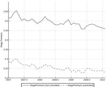
As shown in Figure 3, formal sector wages are 45 to 55% higher than wages in the informal sector. We know, however, that formal and informal sector workers differ in a number of characteristics that affect wages. We then estimate the wage premium in the formal sector
after controlling for observable individual characteristics available in the data.4 Controlled wage
gap is indeed much smaller than the observed one but it is still considerable, ranging from 23 to 30%, as shown in Figure 3. 2007 2007.5 2008 2008.5 2009 2009.5 2010 0.2 0.25 0.3 0.35 0.4 0.45 0.5 0.55 Wage Premium
WagePremium (not controlled) WagePremium (controlled)
Figure 3: Wage Premium
With respect to firm size, while it is not possible to know the exact number of employees in a firm, we are able to divide firm size into three categories: the first one corresponds to firms with 2 to 5 employees, the second one with 6 to 10 employees, and the third with 11 employees or more. Figure 4 presents the averages of these three categories for the informal and formal sectors. Formal sector firms are clearly larger than informal ones.
3
The model
We consider an economy with imperfect competition in the good market and matching frictions in the labor market, populated by a continuum of risk neutral workers whose measure is normalized to unity. There are two sectors, formal (F ) and informal (I), each producing one of the two consumption goods available in the economy.
4We run mincer regressions in cross section for each month, where wages are explained by a dummy for informal
workers, a dummy for each city, and the following worker’s characteristics: age, age square, education, education square, and position in the household.
20032 2004 2005 2006 2007 2008 2009 2010 2.1 2.2 2.3 2.4 2.5 2.6 2.7 2.8 2.9 3 Firms size
Informal Sector Formal Sector Mean
Figure 4: Firm size in formal and informal sectors
3.1 The goods’ market
Households derive utility from consuming goods from both formal and informal sectors, and their preferences are represented by the following utility function:
U = · ασ1 FC σ−1 σ F + α 1 σ IC σ−1 σ I ¸ σ σ−1 (1)
where CF and CI denote a household’s consumption of the good produced in the formal and in
the informal sectors, respectively, while σ stands for the elasticity of substitution between the
two goods. Assuming, for the sake of simplicity, that αF = αI ≡ α, the optimal consumption
pattern of a household n with real income Yn is given by:
Cjn= αYn³ pPj
´−σ
, for j ∈ {F, I}
where pjis the price index of sector j good, P is the composite price index, P =
à α P j=I,F p1−σj !1/(1−σ) , which we normalize to one without loss of generality. There is a continuum of identical consumers in the interval [0, 1], hence aggregate consumption is:
Cj = αY ³ pPj
´−σ
, (2)
where Y ≡R01Yndn denotes aggregate income.
Firms in each sector are identical. In a symmetric equilibrium, they all produce an equal share of the total demand for the sector, hence firms may be labelled only by the industry j they
number or firms in sector j. Nj is fixed in the short run, while in the long run it responds to changes in market profitability and is determined by a free entry condition.
Using equation (2) and the normalization of the aggregate price index, we have that:
pj = µ Njyj αY ¶−1 σ . (3)
In this way, as a result of Cournot competition among firms, the elasticity of demand faced by
a firm in sector j, σj, is positively related to the number of firms operating in that sector as
follows:
σj ≡ σj(Nj) = σNj. (4)
Thus, in this simple framework, we have that the number of firms, Nj, determines the level of
competition in sector j. Several alternative ways to model imperfect competition in the good market can be found in the literature, e.g. Blanchard and Giavazzi (2003), Delacroix (2006), Ebell and Haefke (2009), or Felbermayr and Prat (2010). Our main results would not change substantially when using alternative specifications.
Goods’ production uses labor as sole input. Recent research on informality has highlighted the fact that informal firms are less productive than formal ones. We allow for different produc-tivity across sectors by defining production function as:
yj = Ajhj (5)
where Aj stands for a (sector-specific) productivity parameter and hj is the firm’s size, that
is, the number of workers employed. The size of firms will be endogenously determined in the model. We will see that, in equilibrium, firms in the informal sector are smaller, which is in accordance with the stylized fact described in section 2.
Combining demand function in equation (3) and the production function in (5), goods’ market is in equilibrium when:
NjAjhj = p−σj αY. (6)
3.2 The labor market
Empirical evidence indicates that informal workers have on average lower educational attainment levels (see, among others, Gong and Van Soest, 2002, Gong et al, 2004, and Maloney, 2004).
Since informality would therefore be more a concern for low than for high skill workers5, we
choose to focus on identical workers6 searching for a job in the formal and in the informal sector
5Notice that in the case of developing countries like Brazil, the majority of the population is unskilled.
6This is of course a simplification compared to the papers studying the sorting mechanism between the two
sectors (e.g. Boeri and Garibaldi, 2006, Albrecht et al., 2009), but our focus is not on explaining sorting patterns across sectors.
simultaneously when unemployed. Furthermore, we assume that both formal and informal sectors are subject to matching frictions in the labor market and that they share the same pool of unemployed workers. These two assumptions depart from other recent works that incorporate search-matching frictions to study informality, which assume a segmented labor market and takes the informal sector as a residual perfectly competitive sector.
In each sector, vacant jobs and unemployed workers are brought together in pairs by a
matching function Mj. It maps the number of matches in sector j, Mj, to the total number of
job seekers and vacancies in that sector:
Mj ≡ Mj(u, vj) (7)
where u and vj correspond respectively to the mass of job seekers7, which is the unemployment
rate in the economy, and to the mass of vacancies in the sector. The function Mj features
standard properties: it is twice continuously differentiable, increasing and concave in both of its arguments, it is linearly homogeneous, satisfies the Inada conditions and the boundary conditions
Mj(0, vj) = Mj(u, 0) = 0 for u, vj ≥ 0.
We allow the matching function to be different across sectors to be able to capture their particularities. For instance, firms may rely on different methods to recruit their workers in the two sectors, so that the efficiency of the two matching processes may differ somewhat. It is also often argued that, compared to the formal sector, the informal sector is closer to a competitive market where it takes less time to match. In such a case, the matching process would be more efficient in the informal sector, resulting in a larger number of matches for the same level of inputs in the matching function.
On average, a firm contacts a worker at rate Mj/vj while a job seeker meets a sector j
firm at rate Mj/u. Let θj ≡ vj/u be the labor market tightness. Linear homogeneity of the
matching function allows us to write those contact rates as Mj/vj ≡ mj(θj), with m0j(θj) < 0,
and Mj/u = θjmj(θj), which is an increasing function of θj. Thus vacancies are filled at rate
mj(θj) in sector j while workers exit unemployment at rate
P j=F,I
θjmj(θj).
A few remarks are in order. First, differences in job finding rates between the formal and the informal sector can easily be captured with two matching functions having different scale
parameters. For instance, in the Cobb-Douglas case, MF = κFuηvF1−η while MI = κIuηvI1−η,
with κI ≥ κF. Second, the assumption of search frictions in both sectors encompasses the
particular case of perfect competition in the informal labor market considered in several papers.
That would corresponds to the limit case where κI → ∞ in our framework, i.e. in a fully
7We assume job seekers are ‘truly’ unemployed. Alternatively, we could assume that they are in fact
competitive labor market, where it takes no time to locate a job offer or to fill a vacancy. Finally,
if it took no time to locate a formal job (θFmF(θF) → ∞), all workers would be employed in the
formal sector. Thus, matching frictions are an important reason for the existence of an informal sector, and the underlying assumption for the existence of the two sectors is that the formal sector is ‘sufficiently’ frictional.
Matches are dissolved at rate dj, due either to an exogeneous separation rate sj between
firms and workers or to the exit of firms from the market, which occurs with probability δj.
Hence, the sector-specific destruction rate is:
dj = δj + sj(1 − δj) (8)
Workers can be either employed or unemployed so that:
LF + LI = 1 − u (9)
where Lj = Njhj denotes employment in sector j, and u stands for unemployment. In
steady-state equilibrium, the mass of unemployed workers that find a job in a sector has to equal the mass of workers that loose a job in that sector, that is:
djLj = θjmj(θj)u (10)
Equation (10) states that when a fraction dj of the jobs in sector j are destroyed, they are
compensated by an inflow θjm(θj)u of job seekers who are recruited in sector j.
3.3 Firms’ decisions
Following a growing body of the literature, we depart from the basic matching model by assuming firms can hire more than one worker. This implies that firm size becomes an endogeneous variable which responds to changes in firm’s expected profits. This feature of the model allows us to analyze the determinants of the relative size of firms in the two sectors. In particular, firm size
depends on the elasticity of substitution σj, as we will show below, due to the assumption of
imperfect competition in the good market.
Firms choose the number of vacancies and its size so as to maximize expected profits, which can be written as:
Vj(hj) = max vj,h0j 1 1 + r £ pj(yj) yj(hj) − wj(hj) hj(1 + τj) − γjvj+ (1 − δj) Vj¡h0j¢¤, (11)
where r is the interest rate, γj is the cost of a vacancy, τj represent taxes on labor costs,
in the next section. hj and h0j represent the number of workers in current and next periods,
respectively. The inverse demand function pj(yj) is given by equation (3), while the production
function yj(hj) is in equation (5). Notice that, in this setting, firms do not take prices as given
in the final goods market, as shown by the inverse demand function, and enjoy some bargaining power in the labor market, given by the wage function.
The number of workers next period, h0
j, is determined by the following transition function:
h0j = mj(θj)vj+ (1 − sj)hj, (12)
that is, next period’s employment is equal to the number of matches for the vacancies posted plus the number of current workers that remain employed. Thus, firms advertise as many vacancies as necessary in order to hire, in expected value, the desired number of workers next period,
taking into account the cost of a vacancy γj and the constraints on labor market flows given by
the transition function (12).
The optimal number of vacancies posted is such that the marginal contribution of a worker to the firm’s expected profit is equal to the expected search cost, that is:
(1 − δj)∂Vj(h 0 j) ∂h0 j = γj mj(θj) . (13)
From the profit function (11), the marginal contribution of a worker to the firm’s profit, denoted the envelope condition, can be written as:
∂Vj(hj) ∂hj = 1 1 + r σj− 1 σj pjAj − µ wj(hj) + ∂wj(hj) ∂hj hj ¶ (1 + τj) + (1 − δj) (1 − sj) ∂Vj ³ h0j ´ ∂h0 j , (14)
where we have used the fact that ∂pj(yj)
∂yj ∂yj ∂hjyj+pj ∂yj ∂hj = σj−1 σj pjAjand that ∂h0 j ∂hj = 1−sj. The term σj−1
σj pjAj corresponds to marginal revenue to which the marginal costs
³
wj(hj) +∂w∂hj(hjj)hj ´
×
(1 + τj) of expanding the labor force to hj should be substracted. Marginal costs differs from
wage since firms take into account the effect of an additional worker on the wages of previously employed workers.
In steady state firms’ size is constant, that is, hj = h0
j. Hence, from equation (13) we have
that: ∂Vj(hj) ∂hj = ∂Vj ³ h0j ´ ∂h0j = γj mj(θj) (1 − δj). (15)
Substituting the optimal vacancies condition (13) into equation (14), and using the steady state condition (15), we get that:
pj(hj) = 1 Aj µ σj σj− 1 ¶ ·µ wj(hj) + ∂wj(hj) ∂hj hj ¶ (1 + τj) + γj(r + dj) mj(θj)(1 − δj) ¸ (16)
Equation (16) defines firms’ pricing behaviour in steady state, and can be interpreted as a mark-up equation over total labor costs, inclusive of wage and search costs. Firms enjoy some market power on the good market, but also on the labor market, due to the existence of search
frictions. In the absence of frictions, price pj would simply be equal to 1
Aj ³ σj σj−1 ´ wj. Here,
though, the marginal cost of labor also takes into account the existence of recruitment costs
and the impact of an additional worker on the wages of the infra-marginal workers, ∂wj(hj)
∂hj hj.
The latter term is negative, as shown in next section. This means that employers exploit decreasing marginal returns in order to reduce the wages of each infra marginal worker. For this reason the term is usually denoted in the literature as the overemployment or overhiring effect. Alternatively, equation (16) can be interpreted as a labor demand equation which relates the firms’ optimal employment and wages choices.
Notice that using the steady-state condition that ∂Vj(hj)
∂hj = ∂Vj
³
h0j´ ∂h0j
, the envelope condition
(14) can alternatively be written as:
∂Vj(hj) ∂hj = 1 r + dj · Ajσjσ− 1 j pj− µ wj(hj) +∂w∂hj(hj) j hj ¶ (1 + τj) ¸ , (17)
which will be useful for the derivation of the wage function.
3.4 Wage Bargaining
Let Ej and U denote respectively the asset values of a worker employed in sector j (j ∈ {F, I}) or
searching for a job. An unemployed worker enjoys a flow utility z, which may correspond to e.g. a combination of home-production and/or flow utility from leisure enjoyed while unemployed.
He has a utility gain of (Ej − U ) when he finds a job in sector j, which occurs with probability
θjm (θj). Thus, in steady state we have that:
rU = z + θFm(θF) (EF − U ) + θIm(θI) (EI− U ) (18)
A worker employed in sector j, on his turn, receives a wage wj and incurs an utility loss of
U − Ej when the job is destroyed, which occurs at rate dj. We then have that:
rEj = wj+ dj(U − Ej) (19)
which implies that the benefit of holding a job in sector j over continued search is equal to the
difference between the wage wj and the worker’s reservation product rU, that is:
Ej− U = wr + dj− rU
j . (20)
Workers are not paid their full marginal product as in the standard neoclassical framework due to a combination of costly search and matching frictions which give rise to rent sharing. Most
of the papers which study informality incorporating search frictions assume that wages result from Nash bargaining between one worker and one firm in the sector that experiences search frictions. We assume alternatively that bargaining takes place between a firm and its multiple workers, each worker being treated as the marginal worker. This is a good representation of reality when firms cannot commit to long-term contracts and may renegotiate wages with each worker at any time. This seems an adequate framework to represent a case like the Brazilian one, where job turnover is extremely high (see Gonzaga, 2003).
Furthermore, this interesting alternative assumption has not been implemented yet in the literature studying the composition of employment in terms of formal vs informal jobs. We follow a growing body of the literature that has applied this assumption in studies not related to informality. See, among others, Bertola and Caballero (1994), Stole and Zwiebel (1996), Smith (1999), Cahuc and Wasmer (2001), Delacroix (2006), Cahuc, Marque and Wasmer (2008), Ebell and Haefke (2009), Felbermayr and Prat (2010).
As it will become clear later, bargaining with multiple workers introduces some important dif-ferences compared with the standard one-worker-per-firm framework, as under the neo-classical framework where wages equal marginal product. In particular, this gives rise to an overhiring ex-ternality according to which firms hire workers above the point where the marginal revenue from hiring the marginal worker equals marginal cost, so as to reduce the wage of all inframarginal
workers.8
The bargain between firms and the marginal worker yields:
(1 − βj) (Ej− U ) = βj
1 + τj
∂Vj(hj)
∂hj
. (21)
where βj ∈ [0, 1] can be interpreted as workers’ bargaining power. Using equations (17), (20)
and (21), after some algebra it is possible to show that the wage wj is a solution to the following
differential equation:9 wj(hj) = (1 − βj)rU + βj · Aj 1 + τj σj − 1 σj pj− ∂wj(hj) ∂hj hj ¸ , (22)
which has the following solution:
wj(hj) = (1 − βj)rU + βjσσj− 1 j − βj
Ajpj(hj)
1 + τj . (23)
Equation (23) can be interpreted as the wage curve, which defines the wage as a weighted average of workers’ reservation value rU and of firm’s marginal revenue, captured by the term
σj−1 σj−βj
pj(hj)Aj
1+τj
8Our framework is fairly general, as it always possible to compare the situation where overhiring is ruled out
to the case where it takes place. It is also possible to allow for overhiring in one sector only. This exercise is deferred to section 5.
The relation between wages and employment is clear when one evaluates ∂wj(hj)
∂hj hj.
Combin-ing equations (22) and (23) we get:
∂wj(hj) ∂hj hj = − βj σj− βj | {z } overhiring σj− 1 σj | {z } market power pj(hj)Aj 1 + τj < 0 (24)
which implies that the bargained wage is a decreasing function of employment. It is noticeable from equation (24), that the wage hinges on an overhiring and a market power term. This is due to the fact that the firm’s marginal revenue decreases with the number of workers, since
the increased production from hiring an extra worker tends to reduce the price pj. This effect is
taken into account by the firms enjoying some market power. Given that each worker is treated as the marginal worker, hiring one more worker reduces the wage by
¯ ¯ ¯∂wj(hj) ∂hj ¯ ¯
¯. This leads to the so-called overhiring externality.
Notice that the overhiring effect differs across sectors, since they have different market and bargaining powers. Namely, from equation (24), the overhiring externality increases with
work-ers’ bargaining power βj and decreases with competition σj. It vanishes when βj → 0 or σj → ∞.
In such limit cases, workers are paid a constant wage: they get their reservation wage in the first case, while the marginal product of a worker is constant under full competition in the second. Such limit cases are more likely to apply to the informal sector, since workers’ bargaining power is smaller in the informal sector while competition is more intense than in the formal sector.
We substitute the wage equation (23) and its derivative (24) into the mark-up equation (16) to get: pj = A1 j σj− βj σj− 1 · rU (1 + τj) + 1 − β1 j γj(r + dj) mj(θj)(1 − δj) ¸ , (25)
which establishes the optimal price set by the firm as a function exclusively of variables exogenous to the firm’s decision.
Finally, we substitute price from equation (25) into the wage equation (23) to derive wages also as a function of variables the firm takes as given when taking its decisions:
wj = rU + 1 − ββj
j
γj(r + dj)
mj(θj)(1 − δj)(1 + τj) (26)
Notice that combining equations (16) and (24) we get the equation that determines the optimal employment choice: · wj(hj)(1 + τj) + γj(r + dj) mj(θj)(1 − δj) ¸ σj− βj σj = Ajpj(hj) σj− 1 σj (27)
According to equation (27), firms set employment, and therefore wages, so as to equalize marginal costs to marginal revenue. Marginal revenue, on the right hand side, includes a factor
σj−1
σj < 1, due to their market power in the good’s market. Marginal costs, on the left hand side
of the equation, consist of wages, taxes on labor and expected search costs. It is weighted by
an overhiring factor σj−βj
σj < 1, which establishes that they set hj above the efficient level where
benefit from hiring the marginal worker equals his cost. Firms are willing to do so because they are aware that hiring more workers tends to depress wages paid for their entire workforce. A similar externality is also highlighted in various settings with matching frictions. In our two-sector setting, overhiring should be less important in the two-sector where workers’ bargaining power
βj is smaller or where the elasticity σj is larger. Typically, that should be the case in informal
sectors where there is a larger number of firms and where workers have lower bargaining power10
(see Camargo, 2003).
4
Equilibrium
4.1 Equilibrium in the short-run
We are now ready to determine the short-run equilibrium where the number of firms in each
sector is constant. Given our previous assumptions, having a fixed number of competitors Nj
is equivalent to fixing the elasticity σj faced by each firm in industry j. Hence a short-run
equilibrium is defined for a given value of Nj for each industry, while prices pj, wages wj, firm
size hj and sectoral employment Lj = Njhj, aggregate unemployment u = 1 −
P
j=I,FLj,
tightness θj and workers’ reservation value are endogeneously determined. In the simulations of
the model we do comparative statics analysis to investigate the impact of some of the parameters. In particular, we highlight the impact of fiercer competition on all variables in the short run
by investigating the impact of changes in the degree of competition σj = σNj, captured by a
change in Nj.
Equations (25) and (26) establish optimal prices and wages as a function of labor market tightness and workers’ reservation value. Using the wage bargaining equation (21) and the expression that determines the optimal number of vacancies (13), workers’ reservation value from equation (18) can be rewritten as a function of the labor market tightness, as in:
rU = z + X j=F,I 1 1 + τj βj 1 − βj γjθj 1 − δj. (28)
10Notice that such an externality is here studied assuming that workers’outside options are fixed. Section 5
studies the impact of such a wage bargaining externality when workers’ outside options are endogenous. It is then shown that overhiring in the formal sector may translate into underhiring in the informal sector. In any case, there are reasons to think that the so-called overhiring externality implies a smaller relative size of the informal sector.
With equation (28), the equations for prices (25) and for wages (26) may also be written as
functions of sectoral tightness, as follows:11
pj(θj, θk) = σj− βj σj − 1 1 Aj · (1 + τj) z + 1 + τj 1 + τk βk 1 − βk γkθk 1 − δk + r + dj + βjθjmj(θj) (1 − βj) (1 − δj) γj mj(θj) ¸ , (29) and wj(θj, θk) = z + 1 − ββj j γj(r + dj + θjmj(θj)) (1 − xj) mj(θj) (1 + τj)+ 1 1 + τk βk 1 − βk γkθk 1 − δk (30)
for j, k ∈ {I; F } and k 6= j. It is worth noting that prices and wages in each sector j also depend
on the other sector’s variables, including labor market tightness θk. This is mainly a consequence
of our assumption that workers search employment in both sectors simultaneously, which implies that workers’ reservation value depends on labor market conditions of both sectors as stated by equation (28), while wages and prices are themselves functions of this reservation value.
We now have to determine labor market tightness in the two sectors (θ∗
F, θ∗I). They are determined by the equilibrium conditions in the goods and in the labor markets as follows. First, using equation (6) we get the employment ratio between the informal and formal sectors that satisfy the goods’ market equilibrium. We denote it the product market equilibrium (PME) condition: L∗ I L∗ F = AF AI " pI(θ∗F, θI∗) pF ¡ θ∗ F, θ∗I ¢ #−σ , (31)
which defines implicitly the intersectoral allocation of labor as a function of relative prices and relative productivity, an usual property.
Note that the ratio L∗I/L∗F is a function of tightness θF∗ and θ∗I due to the (positive)
depen-dence of prices pF and pI on these variables, as highlighted by equation (29). A rise in θj∗, would
imply a rise in wages (see equation (26)), translating into a higher price. The quantity consumed thus decreases, resulting in lower employment in the sector. However, as given by (31), the
rela-tive labor allocation L∗
I/L∗F depends on relative (rather than absolute) prices. Since both prices
depend positively on θ∗
F and θI∗, the impact of a change in these variables on relative prices is
ambiguous. It depends on which price is more sensitive to changes in labor market tightness,
which is captured by a condition on price elasticities.12 The comparative statics properties of
this relationship is ambiguous as well, since it depends on which price is impacted the most by
a change in parameters in equation (31).13
11With some abuse of notation, we now write prices and wage as functions of labor market tightness: p
j(θj, θk)
and wj(θj, θk).
12Differentiating (31) we get that the ratio L∗
I/L∗F increases with θ∗I if and only if εpF/θI > εpI/θI. Similarly, the ratio L∗
I/L∗F decreases with θ∗F if and only if εpF/θF < εpI/θF. Nevertheless, such restrictions may not always hold.
13We therefore study the comparative statics on the basis of numerical exercises, and we get monotonic responses
of L∗I
L∗
Second, from equation (10) we derive the relative employment in the two sectors that is compatible with equilibrium in the labor market. We get then the labor market equilibrium (LME) condition: L∗ I L∗ F = dF dI θ∗ ImI(θI∗) θ∗ FmF(θ∗F) . (32)
which defines the intersectoral allocation of labor as a function of sectoral tightness, efficiency parameter of the matching processes and turnover rates. Hence, the LME condition imply that
the informal sector is relatively larger when its own labor market tightness θ∗
I is higher and
when the formal sector’s tightness θ∗
F is lower. Moreover, the formal sector is larger also when
its own destruction rate of jobs is lower and the informal sector’s one is higher.
Equalizing the PME and LME relationships (31) and (32), and making use of the price
equation (29), we determine a first relationship between θ∗
F and θI∗:14 dF dI θI∗mI(θI∗) θ∗ FmF(θ∗F) = AF AI " pI(θ∗F, θI∗) pF ¡ θ∗ F, θI∗ ¢ #−σ (33) Equation (33) establishes the sectoral tightness that satisfy the equilibrium conditions that determine the intersectoral allocation of labor. We then denote it Intersectoral Allocation of Labor curve (IALC).
A second relationship between the two sectoral tightnesses is obtained using the price equa-tion (29) and the definiequa-tion of the aggregate price index:
P∗ = 1 = α1−σ1 £pI(θ∗ I, θ∗F)1−σ+ pF(θ∗I, θ∗F)1−σ ¤ 1 1−σ. We get that: 1 − αpI(θI∗, θ∗F)1−σ = αpF(θ∗I, θF∗)1−σ (34)
which defines a decreasing relationship between θ∗
I and θ∗F. It will be labelled the Price Curve
(PC).
The IALC and PC relationships together determine the equilibrium levels of labor market
tight-ness in the two sectors, θ∗
F and θI∗, by means of a fixed point argument. The equilibrium is unique
provided the IALC relationship evolves monotonically with respect to θ∗
I and θ∗F, as represented
in Figure 5. The numerical simulation in the next section checks this monotonicity, and Figure 13 depicts the corresponding equilibrium.
Once having determined equilibrium values for labor market tightness θ∗
I and θF∗, all other
variables of the model follow: prices p∗
j ≡ pj(θI∗, θ∗F) and wages w∗j ≡ wj(θ∗I, θF∗) are determined
14As mentioned above, the relationship is not necessarily monotonous. We however check in our simulations
6 -θF θI θ∗ F θ∗ I IALC PC
Figure 5: Unique Equilibrium
as a function of tightness in equations (29) and (30). Workers’ reservation product rU∗ is also a
function of tightness as a result from (28). As for sectoral employment levels, the labor market equilibrium conditions (9) and (10) imply:
L∗j = " 1 + dj θ∗ jm(θ∗j) + dj dk θ∗ kmk(θk∗) θ∗ jmj(θ∗j) #−1
, for j, k ∈ {F, I}, and k 6= j (35)
u∗ = 1 − L∗F − L∗I, (36)
and, by definition, v∗
j = θ∗ju∗ while hj∗ = L∗j/Nj, where Nj can be treated as a parameter in the
short run, and will be endogenized in the longer run.
From equation (35), employment in a sector is an increasing function of its own tightness and a decreasing function of the other sector’s tightness. The intuition is the following. If, for
instance, tightness θ∗
j increases in a sector, workers will find jobs in that sector more easily,
thus increasing employment in that sector. Then, from (36), it turns out that unemployment decreases when employment increases in formal or informal sectors.
Finally, in equilibrium total income equals total product, hence:
Y∗= X j=I,F Ajpj ¡ θj∗, θ∗k¢Lj ¡ θj∗, θ∗k¢. (37)
Formal and informal sectors are interdependent for basically two reasons : (i) in equilibrium, demand for goods and therefore sectors’ relative size depend on relative prices, as it is clear from equation (31); (ii) workers search for jobs in both sectors, as established by equation (18). As a
result, a change in sector-specific parameters affects both sectors, as will be shown in the next
section through numerical exercises.15
4.2 Long-run general equilibrium
The next step is to determine the long run equilibrium in which the number of firms in each industry endogenous. The timing of events is the following. At the beginning of a period firms
decide whether enter the market. If they enter they pay an entry cost, cj, on top of the cost of
posting vacancies in a number sufficient to recruit the desired amount of workers.16 Business is
then started and profits are received at the end of that period/begining of the next period. Entry costs entail direct administrative costs as well as indirect costs due to administrative delays. Several of the entry costs do not apply to the informal sector, such as, for instance, the official registration to comply with legislation. Although it would be fair to say that barriers to entry are essentially a problem in the formal sector, informal firms may still incur in entry costs since it may take some time and resources to set up a business in this sector. It is then
reasonable to assume that 0 ≤ cI < cF.
In equilibrium, the free entry condition establishes that the costs of setting a business must equal its profits, as in:
cj+ γjh∗j mj(θ∗ j) = 1 + r r + δjπ ∗ j, for j ∈ {I, F }, (38)
where the second term in the left-hand side corresponds to the cost of posting vacancies to hire
the desired amount of labor h∗
j, and π∗j stands for profits, which is given by:
πj∗ = p∗jAjh∗j − w∗jh∗j(1 + τj) − γjv∗j (39)
= p∗jAjh∗j − w∗jh∗j(1 + τj) − γjsjh∗j/mj(θ∗j).
In the previous section we have derived all short run variables as functions of labor market
tightness θ∗
I and θF∗, which are themselves parameterized by the number of firms operating in
each sector, NI and NF. Hence, in a long run equilibrium, all variables are defined as functions
of NI and NF and equation (38) closes the model .
Firms’ profit opportunities decline with the number of firms operating in the market Nj∗
since with more firms there is more competition and lower markups. Under free entry, a rise in
15The case with identical sectors is studied in the appendix. In that case, the IALC curve becomes the 45oline,
and only the PC curve with θI= θF shifts as parameters change.
16Notice that in our setup, firms jump to their steady state size when they enter the market. This is a
consequence of our assumption of linearity of adjustment costs. See Bertola and Caballero (1994) for a model with convex costs. See also Acemoglu and Hawkins (2010) for an alternative framework where firms cannot hire a large number of workers in each period.
the left hand side of the free entry condition (38), for instance, due to an increase in entry costs
cj or in hiring costs γjh
∗ j
mj(θ∗j) must be compensated by an equal rise of the right hand side of (38),
i.e. higher profits, which is obtained by a smaller equilibrium number of firms.
5
Numerical simulations
5.1 Parametrization and calibration
We choose parameters with two criteria in mind: (i) they have to be realistic and coherent with the values usually used in the literature, (ii) the values of endogeneous variables stemming from the simulations have to be realistic and/or comparable with the values found in previous studies. We choose the Brazilian economy to guide our parametrization. Brazil is a large developing country with a sizeable informal sector, with the advantage of having high quality micro data available, which has already been exploited in a number of empirical studies. Hence, we have both access to data and to other studies that have worked on them.
Our reference period is a month and we use 2003 as reference year. The discount rate r is set to 0.6434% which correspond to an annual rate of 8% as in Heckman and Pag`es (2003). All relevant variables and parameters are allowed to differ between the formal and the informal sectors. Informal sector firms are assumed to be less productive than formal ones, and their pro-ductivity is normalized to one. The propro-ductivity parameter in the formal sector is 2, capturing a productivity differential of 100% between the two sectors, as used by other studies (see, for
instance, Ulyssea, 2009). In terms of our notation, we have then that AF = 2 and AI= 1.
In a recent study, Bartelsman, Haltiwanger, and Scarpetta (2009) estimate that the annual exit rate for Brazilian firm ranges between 5% to 10%, and they indicate that exit rate is higher among smaller firms. Since firms are on average smaller in the informal sector than in the formal one, we use the lower bound of the interval to define firms’ exit rate in the formal sector and, conversely, the upper bound to define firms’ exit rate in the informal sector. It follows that
the monthly values for the two parameters are set to δF = 0.0041 and δI = 0.0080 which is
consistent with the intuition that on average firms’ turnover is higher in the informal sector, i.e.
δF < δI. Labor turnover is higher in the informal sector dF < dI. We choose the parameters to
be equal to dF = 0.0221 and dI = 0.0102 which correspond to an annual rate of 13% and 30%
as in Heckman and Pag`es (2003) and Ulyssea (2009). Finally, making use of equation (8), the
exogenous separation rates are set to sF = 0.0062 and sI = 0.0142 respectively.
The elasticity of the matching function is set to one half, as usual in the literature (Petrongolo and Pissarides, 2001, Shimer, Rogerson and Wright, 2005) while the scale parameter of the
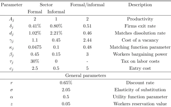
Table 2: Baseline Parameters
Parameter Sector Formal/informal Description
Formal Informal
Aj 2 1 2 Productivity
δj 0.41% 0.80% 0.51 Firms exit rate
dj 1.02% 2.21% 0.46 Matches dissolution rate
γj 1.1 0.45 2.44 Cost of a vacancy
κj 0.0475 0.1 0.48 Matching function parameter
βj 0.45 0.15 3 Workers bargaining power
τj 30% 0 - Tax on labor costs
cj 2.5 0.5 5 Entry cost
General parameters
r 0.65% Discount rate
σ 2.05 Elasticity of substitution
α 0.5 Utility function parameter
z 0.05 Workers reservation value
matching function is set to target an unemployment rate of approximatively 12.5% as in the data (See section 2). According to Camargo (2005) the bargaining power in the informal sector
is approximately 1/3 of that in the formal sector. Those parameters can then be set to βF = 0.45
and βI = 0.15, as in Ulyssea (2009). By definition, the labor tax rate is nil in the informal sector
and we set the formal tax rate equal to 30% which is consistent with the value reported in the World Doing Business Indicators for social security contributions and payroll taxes.
Keeping in mind that firms in informal sectors face lower (if any) entry and flow costs (cF > cI and γF > γI), we set the remaining free parameters so as: (i) to replicate the size
of the informal sector; (ii) to get a reasonable wage premium (wF > wI); (iii) to have a faster
(more efficient) matching process informal sectors (mF(.) < mI(.)); (iv) to have more firms
in the informal sector (NF < NI) but with a lower size (hF > hI). Baseline parameters are
reported in Table 2.
5.2 Results
The result of our numerical exercise matches our targets in terms of aggregate variables, with an unemployment rate around 12% and an informal sector representing 40% of total employment. Wages are approximately 18% higher in the formal sector compared to the informal one, which is roughly consistent with the lower bound of estimated wage differentials between the two sectors,
Table 3: Main endogenous variables
Variable Sector Formal/informal Description
Formal Informal
wj 0.91 0.77 1,18 Wage
θj 0.69 2.18 0.51 Labor market tightness
nj 3.12 5.55 0.46 Number of firms
hj 0.15 0.07 2.44 Firm size
σj 6.40 11.37 0.48 Elasticity of demand for a firm
πj 0.05 0.02 3 Profits
as presented in section 2. Almost similar patterns can be found in Bargain and Kwenda (2009) and Tannuri-Pianto and Pianto (2002) for quantile regressions.
The job finding rate is two times larger in the informal than in the formal sector, which is larger than the differences found in section 2, but is consistent with the viewpoint taken in most existing studies where finding a job in the informal sector is easier than in the formal one (see, e.g. Zenou, 2008, Ulyssea, 2009).
Also consistent with the evidence, there are fewer and larger firms in the formal than in the informal sector as argued in Rauch (1991) and discussed in Tybout (2000). More accurately, we find formal firms to be approximately two times larger than informal ones. Correspondingly, informal firms are approximatively two times more numerous in the informal sector. The re-sulting price elasticity of demand is around 6 in the formal sector compared to about 11 in the informal one. As a consequence, profits are higher in the formal sector. This also means that the aggregate elasticity stands somewhere between those two values. Having different values for the elasticity is a desirable feature of our model. This also means that the various externalities stemming from market and bargaining powers are of different magnitude across sectors. Bench-mark values are summarized in Table 3. In addition, a representation of the equilibrium is given on Figure 13 in Appendix certifying the key IALC condition is monotonic.
5.3 Short run analysis
Competition in the formal sector The number of firms in each sector is fixed in the
short-run. We first examine the impact of a change in the number of firms in the formal sector on the main variables of the model. With this exercice we are able to understand the effect of an exogenous shock on relative competitiveness between the formal and informal sectors. For
each figure, we have depicted two cases: one allowing for overhiring (letting σj−βj
σj < 1, the
σj−βj
σj = 1, the dashed line). We first discuss the case with overhiring, and in the next sub-section
we compare it to the case with no overhiring.
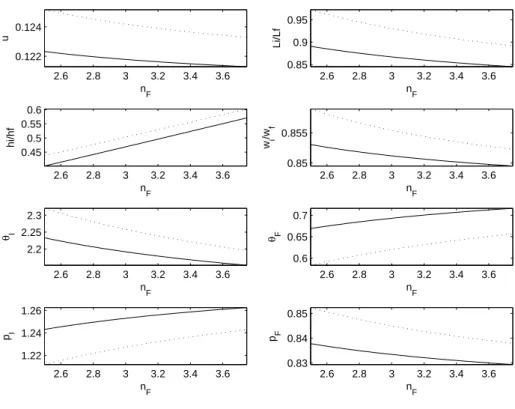
Figure 6 about here
Figures 6 and 7 depict how the economy reacts to an exogenous variation of +/ − 20% of the number of firms in the formal sector compared to the baseline case. The effect is unambiguously (i) a fall in unemployment, though this effect is of moderate magnitude, (ii) a marked rise in the relative size of the formal sector in total employment, though (iii) the relative size of each firm in the formal sector tends to decrease. Finally, it can be seen that (iv) each formal firm pays a relatively higher wage compared to the informal sector when competition in the formal sector becomes fiercer.
Figure 7 about here
These results can be understood by looking at labor market tightnesses and prices. We see that a rise in competition in the formal sector affects tightness in opposite ways across
sectors: tightness increases in the formal sector (θF), while it decreases in the informal sector
(θI). Therefore, this suggests that this is mainly a result of an upward move of the IALC curve
in the (θI, θF) space, assuming that the IALC relationship is monotonically increasing. This
results in a rise in pI and a fall in pF, so that the relative price pI/pF goes up. The increase
in informal sector relative price explains the fall in relative employment in that sector observed
in Figure 6, since LI/LF = (AF/AI) (pI/pF)−σ, from the PME condition (31). In addition, we
see from Figure 7 that this change in relative employment corresponds to a rise in formal sector
employment LF and a fall in informal sector employment LI.
The decrease in the relative size of formal sector firms corresponds to a fall in firm size in
both sectors, as shown in Figure 7. Employment in sector j is equal to Lj = Nj × hj. In
this exercise, the number of firms is fixed in the informal sector. Hence, the fall in sectoral
employment LI translates into a fall in firm size hI. For the formal sector, total employment
LF rises, but so does the number of firms NF. The fact that firm size decreases in that sector
means that the first effect dominates the latter.
Figure 7 also shows that the change in relative wages corresponds to a rise in wages in both
sectors. This is the result of two opposite effects, since θF goes up while θI goes down. We
can therefore conclude that the rise in θF induces a rise in both wages, which dominates the
We can conclude that overall, if the formal sector were more similar to the informal one in terms of the degree of competition, then aggregate employment would be slightly higher while the informal sector would represent a significantly lower share of total employment. Wages would increase in both sectors, with a relatively larger increase in the informal sector. Firms’ profits, however, would be negatively impacted.
The role of wage bargaining externality We now compare the cases with and without
overhiring, when there is an increase in the number of formal sector firms. It turns out that : (i) unemployment is lower in the presence overhiring, compared to the case with no overhiring, as expected. In relative terms, we also see from Figure 6 that the impact of overhiring is larger in the formal sector. (ii) The relative size of the formal sector in total employment is higher, (iii) formal firms are larger and (iv) they pay higher relative wages with overhiring compared to without. Informal firms, on the other hand, are smaller in the presence of overhiring.
These results can be understood by comparing tightnesses and prices with and without overhiring in the previous figures. We see that tightness is larger in the formal sector and lower in the informal sector with overhiring. Otherwise stated, overhiring in the formal sector (θoh
F ≥ θFnooh) translates into underhiring in the informal sector (θohI ≤ θInooh). While the wage
bargaining externality studied in sub-section 3.4 takes place in both sectors, it leads to overhiring in the formal sector, but to underhiring in the informal one, as a result of the interplay between
the two sectors17.
Namely, the opposite moves in θI and θF with and without overhiring suggest that the IALC
curve when overhiring should be above the same curve when overhiring takes place in the (θI, θF)
space.
As a result, the price pI is larger with than without overhiring while the converse holds for
pF, so that the price ratio pI/pF is larger, leading to a smaller relative size of the informal sector
LI/LF = (pI/pF)−σ with than without overhiring as depicted in Figure 8. In a nutshell, the
so-called overhiring externality leads to higher aggregate employment and a lower proportion of informal jobs in total employment.
5.4 Long run analysis
Entry costs We now study the long-run impact of a change in entry costs, in the formal sector
cF, driven by changes in product market regulation for instance, on unemployment u, the share
17Notice that this result contrasts with what would prevail if the two sectors where perfectly identical. Such
a case is studied in the appendix where we show that tightness should be larger in the two sectors with than without overhiring.
of informal employment LI/LF, relative firms’ size hI/hF, and relative wages wI/wF.
An increase in formal sector entry costs would decrease the number of formal sector firms in the long-run. Hence, the long-run impacts of increasing entry costs are very similar qualitatively to the impact of decreasing the number of firms in the formal sector studied in the previous subsection.
Figure 8 about here
The quantitative effects are, however, not exactly the same, since an increase in entry costs in the formal sector reduces the number of firms operating in both sectors, not only in the formal one. As a result, price elasticities decrease for firms in both sectors. This implies that even if the effects do not differ qualitatively between figures 6 and 8, they should be somewhat different in quantitative terms since price elasticities are slightly different. In addition, lower price elasticities also imply larger profits, especially in the formal sector. The impact is then larger on the formal sector than on the informal one, as can be seen from Figure 9 that shows
that relative price elasticity σI/σF = NI/NF increases with entry costs.
Figure 9 about here
This has some noticeable consequences on the labor market. Formal employment decreases with higher entry costs in the formal sector, while informal employment increases. Unemploy-ment, on its turn, increases. From these results, we can conclude that unemployment increases
since the rise in informality is not sufficient to compensate the fall in formal employment.18
Finally, changes in sectoral employment also have an impact on firms’size in each sector:
Overall, it turns out that a decrease in cF, due to e.g. a reduction in product market
regulation strictness, would lead to lower unemployment and a smaller share of informal jobs in total employment. Wages would then be higher in both sectors, with a smaller wage ratio
wI/wF. Notice that the reduction in unemployment and informality in Brazil observed over the
past decade cannot be explained by a lessening of PMR, since it was accompanied by a rise the relative wages in the informal sector.
Bargaining power We now study the long-run impact of a change in workers bargaining
power in the formal sector βF on unemployment u, share of informal employment LI/LF, relative
firms’ size hI/hF, and relative wages wI/wF. Figures 10 and 12 display how the economy reacts
18Notice that while this is true in our numerical exercise, it is not necessarily the case for alternative numerical configurations.