HAL Id: hal-00666681
https://hal-imt.archives-ouvertes.fr/hal-00666681
Submitted on 6 Feb 2012HAL is a multi-disciplinary open access archive for the deposit and dissemination of sci-entific research documents, whether they are pub-lished or not. The documents may come from teaching and research institutions in France or abroad, or from public or private research centers.
L’archive ouverte pluridisciplinaire HAL, est destinée au dépôt et à la diffusion de documents scientifiques de niveau recherche, publiés ou non, émanant des établissements d’enseignement et de recherche français ou étrangers, des laboratoires publics ou privés.
SIR Distribution Analysis in Cellular Networks
Considering the Joint Impact of Path-loss, Shadowing
and Fast Fading
Dorra Ben Cheikh, Jean-Marc Kélif, Marceau Coupechoux, Philippe
Godlewski
To cite this version:
Dorra Ben Cheikh, Jean-Marc Kélif, Marceau Coupechoux, Philippe Godlewski. SIR Distribution Analysis in Cellular Networks Considering the Joint Impact of Path-loss, Shadowing and Fast Fad-ing. EURASIP Journal on Wireless Communications and Networking, SpringerOpen, 2011, 2011 (1), pp.137. �10.1186/1687-1499-2011-137�. �hal-00666681�
SIR distribution analysis in cellular networks
considering the joint impact of path-loss,
shadowing and fast fading
Dorra Ben Cheikh
1,2, Jean-Marc Kelif
1,
Marceau Coupechoux
∗2, and Philippe Godlewski
21
Orange Labs, Issy-les-Moulineaux, France
2TELECOM ParisTech & CNRS LTCI, Paris, France
∗
Corresponding author: coupecho@enst.fr
E-mail addresses:
dorra.bencheikh@orange-ftgroup.com
jeanmarc.kelif@orange-ftgroup.com
coupecho@enst.fr
godlewski@enst.fr
Abstractrandom variables by a log-normal random variable and approximates fast fading coefficients in interference terms by their average value. We denote it FWBM for Fenton-Wilkinson based method. The second one is based on the central limit theorem for causal functions. It allows to approximate a sum of positive random variables by a Gamma distribution. We denote it CLCFM for central limit theorem for causal functions method. Each method allows to establish a simple and easily computable outage probability formula, which jointly takes into account path-loss, shadowing and fast fading. We compute the outage probability, for mobile stations located at any distance from their serving BS, by using a fluid model network that considers the cellular network as a continuum of BS. We validate our approach by comparing all results to extensive Monte Carlo simulations performed in a traditional hexagonal network and we provide the limits of the two methods in terms of system parameters. The proposed framework is a powerful tool to study performances of cellular networks, e.g., OFDMA systems (WiMAX, LTE).
1
Introduction
In this paper, we are interested in characterizing the signal to interference ratio (SIR) distribution on
the downlink of a cellular network. The SIR outage probability and the SIR cumulative distribution
function (CDF) are important metrics for the performance evaluation of wireless communication
systems. In this paper, we define the outage probability as the probability that the SIR at the input
of the receiver chain is falling below a given threshold value. This performance parameter is crucial
for both coverage and capacity studies. In terms of coverage, mobile stations should be able to decode
common control channels (like pilots or broadcast channels) and thus to attain a certain SIR threshold
on these channels with high probability. In this case, we are interested in the low SIR region of the SIR
distribution in order to evaluate the cell coverage. In terms of capacity and for systems implementing
needed for performance evaluation. The ergodic capacity at a certain distance from the base station
is indeed evaluated as an expectation of the Shannon classical formula over the channel variations.
The cell capacity is obtained by integration over the cell area.
The issue of expressing outage probability in cellular networks has been extensively addressed in
the literature. For this study, a difficult task is to take into account the joint impact of path-loss,
shadowing and fast fading. There are two classical assumptions: (1) considering only the shadowing
effect, (2) considering both shadowing and fast fading effects. In the former case, authors mainly
face the problem of expressing the distribution of the sum of log-normally random variables; several
classical methods can be applied to solve this issue (see e.g. [1] [2]). In the latter case, formulas usually
consist in many infinite integrals, which are uneasy to handle in a practical way (see e.g. [3]). In both
cases, outage probability is always an explicit function of all distances from the user to interferers.
As the need for easy-to-use formulas for outage probability is clear, approximations need to be
done. Working on the uplink [4], derived the distribution function of a ratio of path-losses with
shad-owing, which is essential for the evaluation of external interference. For that, authors approximate
the hexagonal cell with a disk of same area. Authors of [5] assume perfect power control on the
uplink, while neglecting fast fading. On the downlink, Chan and Hanly [6] precisely approximate
the distribution of the other-cell interference. They, however, provide formulas that are difficult to
handle in practice and do not consider fast fading. Immovilli and Merani [7] take into account both
channel effects and make several assumptions in order to obtain simplified formulas. In particular,
they approximate interference by its mean value. Outage probability is however an explicit function
of all distances from receiver to every interferer. Zorzi [8], proposes a formula essentially valid for
packet radio networks rather than for cellular systems. Authors of [9] provide some interesting
In this paper, we propose two methods to analyze the outage probability of mobile stations located
at any distance r from their serving base station (BS). The first method, based on the Fenton–
Wilkinson approach [11], approximates a sum of log-normal random variables as a log-normal random
variable and approximates fast fading coefficients in interference terms by their average value. We
denote it FWBM (for Fenton-Wilkinson Based Method). The second one is based on the central limit
theorem for causal functions [12]. It allows to approximate a sum of positive random variables by a
gamma distribution. We denote it CLCFM (for central limit theorem for causal functions method).
Each method allows to establish a simple and easily computable outage probability formula, which
jointly takes into account path-loss, shadowing and fast fading. We compare our proposed formulas
with results obtained with extensive Monte Carlo simulations in a classical hexagonal network. At
last, we rely on fluid model proposed in [13] [14] in order to express the outage probability as a simple
analytical expression depending only on the distance to the serving BS. Such an expression allows
further integrations much more easily than with existing formulas. Note that part of the presented
results are included in [15].
The paper is organized as follows. FWBM is explained in sect. 3. We derive the outage probability
while considering first only path-loss and shadowing and then path-loss, shadowing and fast fading
jointly. Sect. 4 develops the CLCF method. Outage probability is calculated while considering first
only path-loss and fast fading and then path-loss, shadowing and fast fading jointly. The computation
is based on the fluid model (sect. 5). In sect. 6, we validate our approach and compare analytical
2
Interference model
We first define the interference model assumed in this paper. We consider a hexagonal cellular network
with frequency reuse one and we focus on the downlink. We are interested in evaluating the SIR at a
mobile station u, served by base station BS0 and interfered by N interfering base stations. We assume
that mobile stations are attached to their closest BS.
2.0.1 Propagation Model
The power received by u depends on the radio channel state and varies with time due to fading effects
(shadowing and fast fading). Let Pj be the transmission power of base station j, the power pj,u
received by u can be written as:
pj,u= PjKr−ηj,uXj,uYj,u. (1)
The term PjKr−ηj,u, where K is a constant, represents the mean value of the received power at distance
rj,ufrom the transmitter (BSj). Xj,uis a random variable (RV) representing the Rayleigh fading effects,
whose pdf is pX(x) = e−x. The term Yj,u= 10ξj,u/10 is a lognormal RV characterizing shadowing. ξj,u
is a Normal distributed RV, with zero mean and standard deviation, σ, which is typically between 0
and 8 dB. Parameter η, which is typically between 2.7 and 3.5, is the path-loss exponent.
2.0.2 SIR Calculation
The interference power received by a mobile u can be written as:
pext,u = N
X
j=1
that all BS transmit with the same power P0, we can express the SIR expression (dropping index u
and setting r0,u= r):
γ = r −ηX 0Y0 PN j=1r−ηj XjYj . (2) 2.0.3 Outage Probability
In this paper, we define the outage probability as the probability that the SIR at u falls below a given
threshold δ. Note that while varying δ, we obtain the definition of the SIR CDF. In this paper, we
indifferently speak of outage probability or CDF.
P¡γ < δ¢ = P Ã r−ηX 0Y0 PN j=1r−ηj XjYj < δ ! . (3)
3
Fenton-Wilkinson based method
In this section, we propose a first method based on the Fenton-Wilkinson approximation. We first
analyze the path-loss and shadowing impact. We then extend the result to the joint influence of
path-loss, shadowing and fast fading based on the previous obtained result.
3.1
Path-loss and shadowing impact
The power pj received by u can be written in this case:
pj = PjKr−ηj Yj.
The probability density function (PDF) of this slowly varying received power is given by
pY(s) = 1 aσs√π exp " −µ ln(s)√− am 2aσ ¶2#
where a = ln 1010 , m = 1aln(KPjr−ηj ) is the (logarithmic) received mean power expressed in decibels
(dB), which is related to the path-loss and σ is the (logarithmic) standard deviation of the mean
received signal due to the shadowing.
The SIR at user u is now given by:
γ = PNr−ηY0
j=1rj−ηYj
.
We see that the SIR can be written γ = 1/F with
F = N X j=1 r−η j Yj r−ηY0 . (4)
The factor F is defined for any mobile u and it is thus location dependent. The numerator of this factor
is a sum of log-normally distributed RV, which can be approximated by a log-normally distributed
RV [2]. The denominator of the factor is a log-normally distributed RV. F can thus be approximated
by a log-normal RV. Using the Fenton-Wilkinson [11] method, we can calculate the logarithmic mean
and standard deviation, mf and sf of F for any mobile at the distance r from its serving BS, BS0
(see Appendix 1): mf = 1 aln(f (r, η)H(r, σ)), (5) s2 f = 2(σ2− 1 a2 ln H(r, σ)), (6) where H(r, σ) = ea2σ2/2³G(r, η)(ea2σ2 − 1) + 1´− 1 2 , (7)
G(r, η) = P jrj−2η ³ P jr−ηj ´2, (8) f (r, η) = P jr −η j r−η . (9)
From Eqs. (4) and (9), we notice that f (r, η) represents the factor F without shadowing.
The outage probability is now defined as the probability for the SIR γ to be lower than a threshold
value δ and can be expressed as:
P (γ < δ) = 1− Pµ 1δ > F ¶ = 1− P µ 10 log10(1 δ) > 10 log10(F ) ¶ = Q · 10 log10(1δ)− mf sf ¸ . (10)
where Q is the complementary error function: Q(u) = 12erf c(√u 2).
3.2
Path-loss, shadowing and fast fading impact
In this case, the outage probability can be expressed as:
P¡γ < δ¢ = 1 − P Ã r−ηX 0Y0 > δ Ã N X j=1 r−η j XjYj !! .
The interference power received by a mobile u due to fast fading effects varies with time. As
a consequence, the fast fading can increase or decrease the power received by u. We consider that
the increase of interfering power due to fast fading coming from some base stations are compensated
by the decrease of interfering powers coming from other base stations. As a consequence, for the
that ∀j 6= 0, Xj ≈ E[Xj] = 1 (this assumption will be validated by simulations in the next section),
and we can write P¡r−ηX
0Y0 > δ( N P j=1 r−η j XjYj)¢ ≈ P¡r−ηX0Y0 > δ(PNj=1r−ηj Yj)¢. So we have: P¡γ < δ¢ = 1 − P Ã X0Y0 > δ 1 r−η N X j=1 r−η j Yj ! = 1− P¡X0 > δF ¢ = 1− ∞ Z 0 P¡x > δF ¢pX(x)dx = 1− ∞ Z 0 P¡10 log10( x δ) > 10 log10(F )¢e −xdx.
As a consequence, the outage probability for a mobile located at a distance r from its serving BS,
taking into account path-loss, shadowing and fast fading can be written as:
P¡γ < δ¢ = Z ∞ 0 Q ·10 log 10(xδ)− mf sf ¸ e−xdx. (11)
4
Central limit theorem for causal functions method
In this section, we adopt a different path for deriving the SIR CDF. We first express the outage
probability by considering the path-loss and fast fading. Afterwards, we use this result in order to
4.1
Path-loss and fast fading impact
Assuming only fast fading channel, the SIR is given by:
γ = PNr−ηX0 j=1r−ηj Xj = S I, where: S = r−ηX 0, I = N X j=1 r−η j Xj
are two independent RV. To calculate the outage probability, we need to calculate first, the probability
distribution function (PDF) fS(x) of S and the PDF fI(x) of I. The PDF of the useful power is given
by [16]:
fS(x) =
1 r−ηe
−r−ηx .
We now approximate the interference PDF using the central limit theorem for causal functions
[12] by a Gamma distribution given by:
fI(y) =
yν−1
Γ(ν)λνe−
y λ,
where ν = var(I)E[I]2 and λ = var(I)E[I] . Since E[Xj] = 1 and var(Xj) = 1 for j = 1, ..., N , the mean of the
interference power is given by:
E[I] = N X j=1 r−η j E[Xj] = N X j=1 r−η j .
The variance of I can be expressed as:
var(I) = N X j=1 r−2η j var(Xj) = N X j=1 r−2η j .
So we have: ν = ( PN j=1r−ηj )2 PN j=1r−2ηj , (12) λ = PN j=1r−2ηj PN j=1r−ηj . (13)
The outage probability can now be derived as follows:
P(γ < δ) = Z ∞ 0 P(S < Iδ|I = y)f I(y)dy = Z ∞ 0 FS(δy)fI(y)dy. = 1− 1 (r−ηλ δ + 1) ν. (14)
4.2
Path-loss, shadowing and fast fading impact
In this section we will consider that the shadowing follows a log-normal distribution. We can again
write γ = S/I with now
S = r−ηY 0X0, I = N X j=1 r−η j YjXj.
We again approximate the interference PDF using the Central Limit Theorem for Causal Functions.
We thus need to compute the two quantities νs = E[I]
2
var(I) and λs = var(I)
E[I] . Since involved RV are
independent, the average value of I is given by:
E[I] = N X j=1 r−η j E[Yj]E[Xj], = ea2σ22 N X j=1 r−η j .
In the same way, the variance of I is given by: var(I) = N X j=1 r−2η
j ¡E[Yj2]E[Xj2]− E[Yj]2E[Xj]2¢ ,
= ³2e2a2σ2 − ea2σ2´ N X j=1 r−2η j .
The two parameters νs and λs can now be obtained:
νs = 1 2ea2σ2 − 1 ³ PN j=1rj−η ´2 PN j=1r−2ηj , (15) λs = e a2σ2 2 ³ 2ea2σ2 − 1´ PN j=1r−2ηj PN j=1rj−η . (16)
Recall that Y0 follows a log-normal distribution with logarithmic mean 0 and standard deviation
σ. We can thus average the outage probability over the variations of Y0:
P(γ < δ) = Z P(γ < δ|Y0)pY(y)dy, = Z P µ r−ηX 0 < δ yI ¶ pY(y)dy, = 1− Z ∞ 0 1 ( λs r−η δ y + 1)νs × 1 ayσ√2πexp µ −ln(y) 2 2a2σ2 ¶ dy. (17)
5
Analytical fluid model
With the two proposed methods, we obtain expressions of the SIR CDF at a given distance r from
the serving base-station. We see however that expressions depend also on the distances ri between
the considered mobile terminal and all interfering BS. With FWBM, parameters mf and sf in (11)
depend on the ri (see Eqs. (5) and (6)). With CLCFM, parameters νs and λs in (17) depend also on
uneasy to use for dimensioning purposes. In this section, we thus express the parameters mf, sf, νs
and λs as functions dependent only on the distance r using the fluid model.
The fluid model approach has been developed, e.g., in [17]. It consists in replacing on the downlink
a given fixed finite number of transmitters (base stations) by an equivalent continuum of transmitters
which are distributed according to some distribution function. For a homogeneous and regular cellular
network, inteferers are now characterized by the interfering BS density ρBS. Let denote:
g(η) = N X j=1 r−η j . (18)
Assuming an infinite network, the fluid model allows us to approximate g by the following function
[17] (see Appendix 2 for more details). Introducing the dependence of g on r, we obtain:
g(r, η) = 2πρBS
η− 2(2Rc− r)
2−η, (19)
where Rc is the half inter-BS distance.
In the FWBM method, parameters f (r, η) and G(r, η) given by Eqs. (9) and (8), respectively, can
be expressed as follows:
f (r, η) = g(r, η) r−η ,
G(r, η) = g(r, 2η) g(r, η)2.
Parameters mf and sf can thus be written as functions only on the distance r to the serving BS. In
λs = e a2σ2 2 ³ 2ea2σ2 − 1´g(r, 2η) g(r, η) . (21)
6
Performance evaluation
In this section, we compare the figures obtained with analytical expressions (11) and (17) to those
obtained by Monte Carlo simulations. It is clear that several approximations have been done in order
to obtain easy-to-use closed-form formulas: (1) the Fenton-Wilkinson method is known to be accurate
for low standard deviations; (2) the Central Limit Theorem for Causal Functions is an approximation;
(3) the fluid model also. It is thus important to know to what extent approximations are acceptable.
6.1
Monte Carlo simulator
The simulator assumes an homogeneous hexagonal network as the one shown in Fig. 1, made of
fifteen rings around a central cell. The cell range is denoted R, the half-distance between BS is set to
Rc= 1 km.
The simulation consists in computing at each snapshot the SIR for a uniformly random location in
the central cell. This computation can be done independently of the BS output power because noise
is supposed to be negligible both in simulations and analytical study. At each snapshot, shadowing
(log-normal distribution with standard deviation σ) and fast fading (exponential distribution of mean
1) RV are independently drawn between the MS and the serving BS and between MS and interfering
BS. We do not consider correlation between shadowing coefficient. SIR samples at a given distance
from the central BS are recorded in order to compute the outage probability. Five thousand (5,000)
6.2
Results
In this section, we compare obtained formulas with results obtained by Monte Carlo simulations
in a hexagonal network. We study the robustness of our approaches while varying three important
parameters: σ, the standard deviation of the shadowing, η, the path-loss exponent, and r, the distance
to the serving BS.
Moreover, we compare the results for the following approaches:
• SIM: results obtained from Monte Carlo simulations;
• FWBM: the Fenton-Wilkinson Based Method in conjunction with the fluid model;
• CLCFM: the Central Limit Theorem for Causal Functions Method in conjunction with the fluid model;
In Fig. 2, we compare SIR CDF obtained with SIM, FWBM and CLCFM at r = 0.2 Km, for
η = 3.0 and while varying σ from 3 to 8 dB. Parameter σ is definitely the coefficient that influences
the most the difference between analysis and simulations. It is clear that the highest is σ, the highest
is the error induced by approximations. For σ = 8 dB, the CLCFM is not valid anymore if we consider
the whole CDF, but remains accurate for low SIR region. For σ = 3 dB, both methods provide very
accurate results.
In Fig. 3, we study the influence of the distance to the serving BS for σ = 4 dB and η = 3.0. This
distance has a small influence on the accuracy of the proposed methods, all analytical CDF fit well
with the CDF obtained by simulations.
In Fig. 4, we study the path-loss exponent η with fixed σ = 4 dB and distance r = 0.2 km. Here
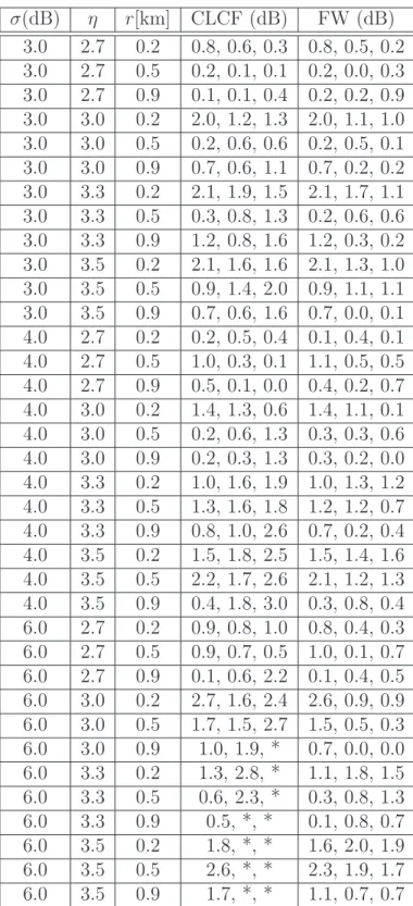
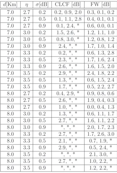
For the sake of completeness, we present in Tables 1 and 2 extensive results for the comparison of
SIM, FWBM, and CLCFM. We set three probability thresholds (5, 50, and 90%) and we obtain the
corresponding SIR thresholds in dB from the different CDF. Reported figures represent the difference
in dB between the threshold obtained with SIM on the one side and the threshold obtained with
FWBM or CLCFM on the other side. Excessive differences (more than 3 dB) are marked with a star.
From these tables, we can draw some conclusions:
• CLCFM provides accurate results for σ ≤ 6 dB and η ≤ 3.0. For all σ ≤ 8 dB, results are still accurate in the low SIR region; this is an interesting result for coverage issues where outage
computations are involved.
• FWBM provides accurate results for σ ≤ 8 dB and η ≤ 3.0, η can be greater if σ is strictly less than 8 dB. At σ = 8 dB and for η ≤ 3.5, results are still accurate in the low SIR region. Theses results show that proposed methods, especially FWBM, can provide accurate results for typical
values of parameters r, σ and η usually considered in cellular networks.
7
Conclusion
In this paper, we establish simple formulas of the outage probability in cellular networks, while
considering loss, shadowing and fast fading. Using FWBM approach, we take into account
path-loss and shadowing to first express the inverse of the SIR of a mobile located at a given distance of
its serving BS as a log-normal random variable. We then consider both path-loss, shadowing and fast
fading and give an analytical expression of the outage probability at a given distance of the serving
BS. Using CLCFM approach, we take into account path-loss and fast fading to express the SIR of
a mobile located at a given distance of its serving BS. We then consider path-loss, fast fading and
BS. The fluid model allows us to obtain formulas that only depend on the distance to the serving
BS. The analytical model that we propose is validated by comparisons with Monte Carlo simulations.
The formulas derived in this paper allow to obtain performances results instantaneously.
The proposed framework is a powerful tool to study performances of cellular networks and to
design fine algorithms taking into account the distance to the serving BS, shadowing and fast fading.
It can particularly easily be used to study frequency reuse schemes in OFDMA systems.
Appendix 1
In this section, we derive the logarithmic mean and standard deviation of F (see equation (4)) using the
Fenton-Wilkinson method. Several classical techniques exist in the literature in order to approximate
a sum of log-normal RV, e.g., Schwartz-Yeh [18] and Farley [19]. The former needs complex recursive
calculations, the latter assumes identical mean and standard deviation. On the contrary, the
Fenton-Wilkinson method provides a closed-form formula for non identical distributed log-normal RV.
Each term of the sum in the numerator of F is a RV following a log-normal distribution. We can
write ln(r−η
j Yj)∝ N (amj, a2σ2), where a = ln(10)/10 and mj = 1aln(r−ηj ). The sum S =
PN
j=1rj−ηYj
can itself be approximated by a log-normal RV: ln(S)∝ N (am, a2σ2
s) with: am = ln à N X j=1 eamj ! + a 2σ2 2 − a2σ2 s 2 , a2σs2 = ln ³ ea2σ2 − 1´ PN j=1e2amj ³ PN j=1eamj ´2 + 1 .
a2σ2s = ln ³ ea2σ2 − 1´ PN j=1r−2ηj ³ PN j=1r−ηj ´2 + 1 .
Taking now into account the denominator, the logarithmic mean value of F is simply amf = am−
(−η ln(r)) and the logarithmic standard deviation of F is a2s2
f = a2σ2s + a2σ2. The ratio of two
log-normal RV is indeed a log-log-normal RV with mean, the difference of the means, and variance, the sum
of the variances. With the definitions of f , G and H, we obtain Eqs. (5) and (6). Note that mf and
sf are expressed in dB.
Appendix 2
In this section, we shortly recall the fluid model approach, that will allow us to simplify Eq. 18.
The fluid model approach consists of replacing a given fixed finite number of interfering BS by an
equivalent continuum of transmitters which are uniformly distributed with density ρBS.
We consider a central cell and a round shaped network around this cell with radius Rnw. The
inter-site distance is 2Rc (see Fig. 5). Let’s consider a mobile u at a distance ru from its serving
BS. In the fluid model, each elementary surface zdzdθ at a distance z from u contains ρBSzdzdθ BS
which contribute to function g. Their contribution to the sum over j is ρBSzdzdθz−η (η > 2). We
approximate the integration surface by a ring with centre u, inner radius 2Rc− ru, and outer radius
Rnw− ru (see Fig. 6): g(ru, η) = Z 2π 0 Z Rnw−ru 2Rc−ru ρBSz−ηzdzdθ, = 2πρBS η− 2 £(2Rc− ru)2−η− (Rnw− ru)2−η¤ . (22)
If the network is large, i.e., Rnw is big in front of Rc, g can be further approximated by (dropping subscript u): g(r, η) = 2πρBS η− 2(2Rc− r) 2−η. (23)
Competing Interests
The authors declare that they have no competing interest.
References
[1] M Pratesi, F Santucci, F Graziosi, M Ruggieri, Outage analysis in mobile radio systems with
generically correlated log-normal interferers. Commun. IEEE Trans. 48(3):381 –385, (2000)
[2] GL Stuber, Principles of Mobile Communications, 2nd Ed. (Kluwer Academic Publishers,
Boston/Dordrecht/London, 2001)
[3] J-PMG Linnartz, Exact analysis of the outage probability in multiple-user mobile radio. Commun.
IEEE Trans., 40(1):20 –23 (1992)
[4] JS Evans, D Everitt, Effective bandwidth-based admission control for multiservice cdma cellular
networks. Vehi. Technol., IEEE Trans. 48(1):36 –46 (1999)
[5] VV Veeravalli, A Sendonaris, The coverage-capacity tradeoff in cellular cdma systems. Vehi.
Technol., IEEE Trans. 48(5):1443 –1450 (1999)
[6] CC Chan, SV Hanly, Calculating the outage probability in a cdma network with spatial poisson
[7] G Immovilli, ML Merani, Simplified evaluation of outage probability for cellular mobile radio
systems. Electronics Letters 27(15):1365 –1367 (1991)
[8] M Zorzi, S Pupolin, Outage probability in multiple access packet radio networks in the presence
of fading. Vehi. Technol., IEEE Trans. 43(3):604 –610 (1994)
[9] J Papandriopoulos, J Evans, S Dey, Outage-based optimal power control for generalized multiuser
fading channels. Commun., IEEE Trans. 54(4):693 – 703 (2006)
[10] AG Williamson, JD Parsons, Outage probability in a mobile radio system subject to fading and
shadowing. Electronics Lett. 21(14):622 –623 (1985)
[11] L Fenton, The sum of log-normal probability distributions in scatter transmission systems.
Com-mun. Sys., IRE Trans. 8(1):57 –67 (1960)
[12] A Papoulis, The Fourier Integral and Its Applications. (McGraw-Hill, New York, 1962)
[13] J-M Kelif, Admission control on fluid cdma networks, in Modeling and Optimization in Mobile,
Ad Hoc and Wireless Networks, 2006 4th International Symposium on, pp. 1 – 7, Apr. 2006.
[14] J-M Kelif, E Alman, Downlink fluid model of cdma networks. In Vehicular Technology Conference,
2005. VTC 2005-Spring. 2005 IEEE 61st, volume 4, pages 2264 – 2268 Vol. 4, May 2005.
[15] JM Kelif, Marceau Coupechoux, Joint impact of pathloss shadowing and fast fading - an outage
formula for wireless networks. ArXiv, abs/1001.1110, 2010.
[16] MK Simon, M-S Alouini, Digital Communication Over Fading Channels. (John Wiley & Sons,
Hoboken, New Jersey, 2005)
[17] J-M Kelif, M Coupechoux, P Godlewski, Spatial outage probability for cellular networks, in
[18] S Schwartz, YS Yeh, On the distribution function and moments of power sums with log-normal
components. Bell Syst. Tech. J., 61:1441-1462 (1982)
[19] NC Beaulieu, AA Abu-Dayya, PJ McLane, Comparison of methods of computing lognormal
sum distributions and outages for digital wireless applications, in International Conference on
Communications, ICC, May 1994.
Figure 1: Hexagonal network and main parameters of the study: the cell range R, the inter-site distance 2Rc and the network size Rnw.
Table 1: CDF difference in dB between Monte Carlo simulations (SIM) on the one hand and CLCFM and FWBM on the other hand at 5, 50 and 90% (σ =3, 4, 6 dB, * means greater than 3 dB).
σ(dB) η r[km] CLCF (dB) FW (dB) 3.0 2.7 0.2 0.8, 0.6, 0.3 0.8, 0.5, 0.2 3.0 2.7 0.5 0.2, 0.1, 0.1 0.2, 0.0, 0.3 3.0 2.7 0.9 0.1, 0.1, 0.4 0.2, 0.2, 0.9 3.0 3.0 0.2 2.0, 1.2, 1.3 2.0, 1.1, 1.0 3.0 3.0 0.5 0.2, 0.6, 0.6 0.2, 0.5, 0.1 3.0 3.0 0.9 0.7, 0.6, 1.1 0.7, 0.2, 0.2 3.0 3.3 0.2 2.1, 1.9, 1.5 2.1, 1.7, 1.1 3.0 3.3 0.5 0.3, 0.8, 1.3 0.2, 0.6, 0.6 3.0 3.3 0.9 1.2, 0.8, 1.6 1.2, 0.3, 0.2 3.0 3.5 0.2 2.1, 1.6, 1.6 2.1, 1.3, 1.0 3.0 3.5 0.5 0.9, 1.4, 2.0 0.9, 1.1, 1.1 3.0 3.5 0.9 0.7, 0.6, 1.6 0.7, 0.0, 0.1 4.0 2.7 0.2 0.2, 0.5, 0.4 0.1, 0.4, 0.1 4.0 2.7 0.5 1.0, 0.3, 0.1 1.1, 0.5, 0.5 4.0 2.7 0.9 0.5, 0.1, 0.0 0.4, 0.2, 0.7 4.0 3.0 0.2 1.4, 1.3, 0.6 1.4, 1.1, 0.1 4.0 3.0 0.5 0.2, 0.6, 1.3 0.3, 0.3, 0.6 4.0 3.0 0.9 0.2, 0.3, 1.3 0.3, 0.2, 0.0 4.0 3.3 0.2 1.0, 1.6, 1.9 1.0, 1.3, 1.2 4.0 3.3 0.5 1.3, 1.6, 1.8 1.2, 1.2, 0.7 4.0 3.3 0.9 0.8, 1.0, 2.6 0.7, 0.2, 0.4 4.0 3.5 0.2 1.5, 1.8, 2.5 1.5, 1.4, 1.6 4.0 3.5 0.5 2.2, 1.7, 2.6 2.1, 1.2, 1.3 4.0 3.5 0.9 0.4, 1.8, 3.0 0.3, 0.8, 0.4 6.0 2.7 0.2 0.9, 0.8, 1.0 0.8, 0.4, 0.3 6.0 2.7 0.5 0.9, 0.7, 0.5 1.0, 0.1, 0.7 6.0 2.7 0.9 0.1, 0.6, 2.2 0.1, 0.4, 0.5 6.0 3.0 0.2 2.7, 1.6, 2.4 2.6, 0.9, 0.9 6.0 3.0 0.5 1.7, 1.5, 2.7 1.5, 0.5, 0.3 6.0 3.0 0.9 1.0, 1.9, * 0.7, 0.0, 0.0 6.0 3.3 0.2 1.3, 2.8, * 1.1, 1.8, 1.5 6.0 3.3 0.5 0.6, 2.3, * 0.3, 0.8, 1.3 6.0 3.3 0.9 0.5, *, * 0.1, 0.8, 0.7 6.0 3.5 0.2 1.8, *, * 1.6, 2.0, 1.9 6.0 3.5 0.5 2.6, *, * 2.3, 1.9, 1.7 6.0 3.5 0.9 1.7, *, * 1.1, 0.7, 0.7
Figure 3: Influence of the distance to the serving BS r [km] with σ = 4 dB and η = 3.0.
Table 2: CDF difference in dB between Monte Carlo Simulations (SIM) on the one hand and CLCFM and FWBM on the other hand at 5, 50 and 90% (σ =7 and 8 dB, * means greater than 3 dB).
d[Km] η σ[dB] CLCF [dB] FW [dB] 7.0 2.7 0.2 0.2, 0.9, 2.0 0.3, 0.1, 0.2 7.0 2.7 0.5 0.1, 1.1, 2.8 0.4, 0.1, 0.1 7.0 2.7 0.9 0.1, 2.4, * 0.6, 0.0, 0.1 7.0 3.0 0.2 1.5, 2.6, * 1.2, 1.1, 1.0 7.0 3.0 0.5 0.8, 3.0, * 1.2, 0.8, 1.2 7.0 3.0 0.9 2.4, *, * 1.7, 1.0, 1.4 7.0 3.3 0.2 0.2, *, * 0.6, 1.3, 2.8 7.0 3.3 0.5 2.3, *, * 1.7, 1.6, 2.4 7.0 3.3 0.9 2.6, *, * 1.6, 1.5, 2.0 7.0 3.5 0.2 2.9, *, * 2.4, 1.8, 2.2 7.0 3.5 0.5 1.3, *, * 0.6, 1.5, 2.4 7.0 3.5 0.9 1.7, *, * 0.5, 2.2, 2.7 8.0 2.7 0.2 0.4, 2.9, * 0.9, 0.8, 0.6 8.0 2.7 0.5 2.6, *, * 1.9, 0.4, 0.3 8.0 2.7 0.9 1.0, *, * 0.0, 0.4, 1.3 8.0 3.0 0.2 1.3, *, * 0.6, 1.1, 1.7 8.0 3.0 0.5 2.7, *, * 1.6, 1.1, 2.2 8.0 3.0 0.9 *, *, * 2.0, 1.7, 2.3 8.0 3.3 0.2 2.7, *, * 1.7, 2.6, 3.0 8.0 3.3 0.5 2.1, *, * 0.7, 1.9, * 8.0 3.3 0.9 2.9, *, * 0.5, 2.4, * 8.0 3.5 0.2 *, *, * 2.1, 3.0, * 8.0 3.5 0.5 2.7, *, * 1.0, 2.2, * 8.0 3.5 0.9 *, *, * 1.2, 2.2, *
Figure 5: Network and cell of interest in the fluid model; the distance between two BS is 2Rc and the
network is made of a continuum of base stations.
−200 −10 0 10 20 30 40 0.1 0.2 0.3 0.4 0.5 0.6 0.7 0.8 0.9 1 SIR threshold [dB] σ = 8 dB CLCFM FWBM SIM −200 0 20 40 0.1 0.2 0.3 0.4 0.5 0.6 0.7 0.8 0.9 1 SIR threshold [dB] σ = 6 dB −200 0 20 40 0.1 0.2 0.3 0.4 0.5 0.6 0.7 0.8 0.9 1 SIR threshold [dB] σ = 4 dB −200 0 20 40 0.1 0.2 0.3 0.4 0.5 0.6 0.7 0.8 0.9 1 SIR threshold [dB] σ = 3 dB
0.1 0.2 0.3 0.4 0.5 0.6 0.7 0.8 0.9 1 r = 0.9 Km CLCFM FWBM SIM 0.1 0.2 0.3 0.4 0.5 0.6 0.7 0.8 0.9 1 r = 0.5 Km 0.1 0.2 0.3 0.4 0.5 0.6 0.7 0.8 0.9 1 r = 0.2 Km
−200 −10 0 10 20 30 40 0.1 0.2 0.3 0.4 0.5 0.6 0.7 0.8 0.9 1 SIR threshold [dB] η = 3.5 CLCFM FWBM SIM −200 −10 0 10 20 30 40 0.1 0.2 0.3 0.4 0.5 0.6 0.7 0.8 0.9 1 SIR threshold [dB] η = 3.0 −200 −10 0 10 20 30 40 0.1 0.2 0.3 0.4 0.5 0.6 0.7 0.8 0.9 1 SIR threshold [dB] η = 2.7