On the impact of mobility in cellular networks

(1)

On the impact of mobility in cellular networks

Elene Anton

¹

, Urtzi Ayesta

^1,2

, and Florian Simatos

^3,4

1

CNRS, IRIT, 2 rue Charles Camichel, 31071 Toulouse, France

2

IKERBASQUE - Basque Foundation for Science, 48011 Bilbao, Spain

3

ISAE Supaero, 10 avenue ´ Edouard-Belin, 31055 Toulouse, France

4

Université Fédérale de Toulouse, 41 Allées Jules Guesde, 31013 Toulouse, France

Abstract—It is well-known that mobility increases the throughput of wireless networks, and the main objective of this paper is to show that, depending on the system’s parameters, delay can actually be negatively impacted. To do so, we study a Markovian model where users arrive to the network according to a Poisson process with rate λ and then move at speed α ∈ [0, ∞) between nodes while in service.

Given the complexity of the model, we resort to approximation techniques in order to get insight into the influence of the speed α on the mean delay. Our main findings are the following:

•

in the case where the network consists of two nodes, delay is monotone in α for small values of λ. We furthermore explicit a constant C such that delay is increasing if and only if C < 0;

•

in the general case, we provide numerical results showing that delay is not necessarily monotone in α. However, we compare the two extreme cases with 0 and infinite speed, and find that for small values of λ, delay is worse with infinite speed than with 0 speed if and only if C < 0.

Finally, an intuitive interpretation of this constant C is provided.

Index Terms—wireless network, mobility, impact, performance

I. I

NTRODUCTION

The impact of mobility in the performance of communica- tions systems has attracted considerable attention from the research community. In a seminal paper, Grossglauser and Tse [1] showed that in an ad-hoc network, the capacity of the network increases in the case nodes move. Since then, the impact of mobility has been studied in many other papers, see for instance [1]–[5]. Among the different examples, Bonald et al. [2], consider a wireless system carrying elastic traffic from different classes. Service is provided according to a set of feasible service rate vectors that depends on the active user population in a fairly intricate fashion due to channel- scheduling. Mobility is modulated by introducing a speed parameter in this set of feasible service rate vectors. It is proven that the mean response time is lower (upper) bounded by the system with speed infinity (zero), which implies that mobility always improves the performance of the system. In spite of the differences across the models studied, all previous analysis led to the conclusion that mobility improves the performance of the system.

In this paper we aim at assessing the impact of mobility on the performance as perceived by users. In order to do so, we consider the same open queueing network that was recently studied by Ganesh et al. in [6]. They consider a K parallel

server system where new jobs arrive to node i according to a Poisson process of rate λp

i

, where λ is the total arrival rate to the system and p

i

is the fraction of jobs that start in node i, service time requirements are exponentially distributed with unit mean, jobs complete service at node i with an exponential rate µ

i

, and jobs from node i move to node j with an exponential rate αr

ij

. The case α = 0 corresponds to the case in which there is no mobility, and as α increases, the rate of mobility of every job increases.

For this model, the impact of mobility on stability from a queueing perspective is easy to understand and quantify, i.e., mobility connects otherwise disconnected nodes, the load distributes across the network, and the stability region increases. Thus, with α = 0, there is no mobility, and all nodes need to be stable separately, the stability condition of the system is max

_i

{λp

_i

− µ

_i

} < 0. However, for any α > 0, the network becomes interconnected, and in [6] it was shown that the stability condition upgrades up to P

i

λp

i

< P

i

µ

i

. The above results imply that mobility improves the throughput, but it does not provide insights regarding whether mobility improves the quality of service as perceived by users. We answer this question negatively, and we provide, to the best of our knowledge, the first rigorous evidence that mobility may negatively impact delay performance. In contrast to prior works such as [2], we prove that under certain conditions, mobility might induce an increase in the service time. To achieve this goal, we analyze the mean number of jobs in the system, which by Little’s law, is proportional to the mean delay as perceived by users. Given the complexity of the model, exact analysis of steady state performance is not possible. We thus study the light traffic regime, i.e., when λ ≈ 0, and consider two metrics to assess the performance:

(i) for any given α < ∞, the mean number of jobs in the system, and (ii) the difference in the number of jobs between the extreme cases in which α is either 0 or ∞. For both measures, we obtain a sufficient set of conditions depending on the model parameters, such that for sufficiently low λ (i) the mean number of jobs decrease in, and (ii) the difference in the mean number of jobs for the extreme values of is negative.

To analyze the model when α → ∞ we prove that the

sequence of stationary distributions converge to an explicit

limit which can be decomposed into a one-dimensional birth-

and-death process describing the total number of users in

system, and a multinomial distribution describing how these

(2)

users are distributed among the servers.

The rest of the paper is organized as follows. In Section III we analyse the light traffic approximation of the mean number of jobs with respect to the mobility parameter. In Section IV we consider the system outside the light traffic regime; we define the system as α → ∞ and analyse the difference in the mean number of jobs for the systems with α = 0 and α = ∞.

Section V presents numerical results.

II. M

ODEL DESCRIPTION

Our basic model is a K parallel server open queueing network in which a job might move among the servers while receiving service. As already mentioned in the introduction, jobs have an exponentially distributed service requirement with unit mean and arrive to the network according to a Poisson process of rate λ. For any server i, i = 1, . . . , K, let p

i

, µ

i

, λ

i

:= λp

i

denote the fraction of jobs that start in node i, its speed, and its arrival rate respectively. We note that P

K

i=1

p

i

= 1. We let µ ¯ = P

i

µ

i

denote the sum of the capacities of each server.

A job in server i, i = 1, . . . , K, moves to server j with an exponential rate αr

ij

, where α is the parameter that controls the moving speed. Thus, while in the network users move according to the Q-matrix αR = (αr

ij

)

i,j

We assume that the corresponding irreducible Markov chain is independent across jobs and we denote by ~ π = (π

1

, . . . , π

K

) its unique stationary distribution. We note that ~ π does not depend on α.

The state of the system at time t ≥ 0 is given by the number of jobs present at each server, N ~

^α

(t) = (N

₁^α

(t), . . . , N

_K^α

(t)).

The non-zero components in the transition matrix of the process N ~

^α

(t) are given by:

Q

^α

(~ n, ~ m) =



 



 



λp

_i

, if m ~ = ~ n + ~ e

_i

, for i = 1, . . . , K

µ

_i

, if m ~ = ~ n − ~ e

_i

and n

^α_i

> 0, for i = 1, . . . , K

αn

i

r

ij

, if m ~ = ~ n + ~ e

j

− ~ e

i

for i, j = 1, . . . , K, i 6= j where ~ n, ~ m ∈ N

^K

and ~ e

_i

= (0, . . . , 0, 1, 0, . . . , 0) ∈ R

^K

, with a 1 in the i−th position. Note that λp

_i

(µ

_i

) corresponds to an arrival to (a departure from) server i. Each job in server i moves into server j at rate αr

_ij

, hence, the total moving rate from server i to sever j is αn

i

r

ij

.

From the stability viewpoint, with α = 0, there is no mobility, and all nodes need to be stable separately, and the stability condition of the system is max

_i

{λp

_i

− µ

_i

} < 0.

On the other hand for any α > 0, the network becomes interconnected, and in [6] it was shown that the stability condition becomes λ < µ. Thus, the stability region with ¯ mobility is always larger than in the case without mobility.

We will denote by ρ = λ/¯ µ the load in the system.

Whenever the stability condition for given α ≥ 0 holds, we let ~ Π

^α

= (Π

^α

(n))

_n∈_ZK

+

denote the steady-state distribution of

N ~

^α

(t). From theory, we know that Π ~

^α

is the unique solution of the balance equations given by:

λΠ

^α

( ~ 0) =

K

X

i=1

µ

_i

Π

^α

(~ e

_i

), (1) and for states ~ n 6= ~ 0







K

X

i=1

λp

i

+

K

X

i,j=1 i6=j

αn

i

r

ij

+

K

X

i=1

µ

i

1(n

i

> 0)





 Π

^α

(~ n)

=

K

X

i=1

(λp

_i

Π

^α

(~ n − ~ e

_i

)1(n

_i

> 0) + µ

_i

Π

^α

(~ n + ~ e

_i

))

+

K

X

i,j=1 i6=j

(n

_j

+ 1)αr

_ji

Π

^α

(~ n + ~ e

_j

− ~ e

_i

)1(n

_i

> 0) (2)

where 1(·) denotes the indicator function.

Our main performance measure is the mean number of jobs in steady state, which by Little’s law is proportional to the mean delay. We denote by N ~

^α

(∞) a random variable distributed as Π ~

^α

.

III. M

ONOTONICITY IN THE LIGHT TRAFFIC REGIME FOR

K = 2

The light-traffic approximation corresponds to the first- order asymptotic expansion of the system as λ → 0, see [7]

for more details. More precisely, as λ → 0 we seek to write E(| N ~

^α

(∞)|) = λm

^LT

(α) + o(λ) for some m

^LT

(α) > 0.

To find this expansion, the idea is to neglect states with two or more users, as these states will become negligible in the limit λ → 0. Indeed, when λ 1, starting empty the system evolves as follows: for a long duration, of the order of 1/λ, nothing happens. Then, an arrival occurs. The user typically stays in the system for a O(1) duration during which no new arrival occurred, since it typically occurs after a duration of the order of 1/λ. Thus, states with two or more users are exceptional and can be neglected.

The light traffic analysis of general K is cumbersome, we thus focus on the K = 2 case. However, as we will see later, this provides interesting insights on the performance of the system. Neglecting states with two or more users, the balance equations (1) and (2), simplify into the following system of equations:

λΠ

^α,LT

(0, 0) = µ

1

Π

^α,LT

(1, 0) + µ

2

Π

^α,LT

(0, 1) (µ

₁

+ αr

₁₂

)Π

^α,LT

(1, 0) = λp

₁

Π

^α,LT

(0, 0) + αr

₂₁

Π

^α,LT

(0, 1) (µ

₂

+ αr

₁₂

)Π

^α,LT

(0, 1) = λp

₂

Π

^α,LT

(0, 0) + αr

₁₂

Π

^α,LT

(1, 0) (3) By solving these balance equations we obtain the following results:

Π

^α,LT

(0, 0) =

_λ(α(r ^α(µ¹^r²¹^+µ²^r¹²^)+µ¹^µ²

12+r₂₁)+p₁µ₂+p₂µ₁)+α(µ₁r₂₁+µ₂r₁₂)+µ₁µ₂

Π

^α,LT

(1, 0) =

_λ(α(r ^λ(αr²¹^+p¹^µ²⁾

12+r21)+p1µ2+p2µ1)+α(µ1r21+µ2r12)+µ1µ2

Π

^α,LT

(0, 1) =

_λ(α(r ^λ(αr¹²^+p²^µ¹⁾

12+r21)+p1µ2+p2µ1)+α(µ1r21+µ2r12)+µ1µ2

(3)

which gives, as λ → 0, (here ≈ has an informal sense, while

∼ is the usual leading asymptotic term)

E(| N ~

^α

(∞)|) ≈ Π

^α,LT

(1, 0) + Π

^α,LT

(1, 0) ∼ λm

^LT

(α) with

m

^LT

(α) = α +

^p_(r¹^µ²^+p²^µ¹

12+r₂₁)

α(µ

1

π

1

+ µ

2

π

2

) +

_(r^µ¹^µ²

12+r₂₁)

(4) where in this simple 2-node case we have π

1

=

_r ^r²¹

12+r₂₁

and π

2

=

_r ^r¹²

12+r₂₁

.

As announced in the introduction and discussed in more details below, one of our main finding is that delay performance is not necessarily monotone, let it increasing, with the speed of users. However, at least in the case K = 2, the previous result actually shows that delay is monotone in the light traffic regime. Moreover, it can be increasing or decreasing depending on the precise parameters as shown below.

Proposition 3.1: If µ

₁

= µ

₂

or p

₁

π

₂

µ

₂

= p

₂

π

₁

µ

₁

, then m

^LT

is constant. If µ

₁

> µ

₂

, then m

^LT

is strictly increasing if p

₁

π

₂

µ

₂

> p

₂

π

₁

µ

₁

and strictly decreasing if p

₁

π

₂

µ

₂

< p

₂

π

₁

µ

₁

.

Proof: This result comes from the expression of the derivative of m

^LT

in α, namely

d

dα m

^LT

(α) = (µ

₁

− µ

₂

)(p

₁

π

₂

µ

₂

− p

₂

π

₁

µ

₁

) (r

12

+ r

21

)

α(µ

1

π

1

+ µ

2

π

2

) +

_(r^µ¹^µ²

12+r₂₁)

2

These conditions can be put in a more concise form as follows. Let in the sequel

C :=

K

X

i=1

p

i

µ

_i

!

− 1

P

K

i=1

µ

_i

π

_i

(5) Then, in the case K = 2 and µ

1

> µ

2

, the above result can be restated by saying that m

^LT

is strictly increasing if C < 0 and strictly decreasing if C > 0. This result has a nice interpretation. The first term in C is the mean sojourn time of a user arriving to the network if it were not to move, while the second term is the mean sojourn time of a user moving at infinite speed. Thus C < 0 means that a user would depart sooner by not moving because it is more likely to have arrived to a favorable node, and so in this case mobility should worsen the system’s performance, which is indeed the content of Proposition 3.1 since in this case m

^LT

is increasing with α. It is interesting that, in the light traffic regime, only the two extreme cases with zero and infinite speeds matter. The comparison between these two extreme cases is the purpose of the next section.

In Section V we show some examples to illustrate the behaviour of E(| N ~

^α

(∞)|) outside the light traffic regime.

IV. G

ENERAL CASE

:

COMPARISON OF THE

α = 0

AND

α = ∞

CASES

The constant C introduced above suggests to compare the case without mobility to the case with infinity mobility outside the light traffic regime, which is what we do here. The main

difference with the preceding section is that we do not restrict ourselves to the case K = 2. To do so, we assume that λ

i

< µ

i

for every i, so that the systems with and without mobility are stable, and we compare the two extreme cases α = 0 and α = ∞ through the metric

∆ := E(| N ~

⁰

(∞)|) − E(| N ~

^∞

(∞)|).

In order to give sense to this metric, we first explain what we mean by the case α = ∞ and we intuitively define what should be the process, which we denote by N ~

^∞

, in this regime. We then show convergence as α → ∞ of N ~

^α

to N ~

^∞

in a suitable sense, namely in the sense of finite-dimensional distributions and also the stationary distributions.

A. The system with infinite speed

Here we define the limiting process N ~

^∞

corresponding to infinite speed. As the speed of mobility increases, the dynamics within the system can be decomposed into two types. On a relatively slow time scale, the total number of jobs changes due to an arrival or a departure, whereas on a relatively fast time scale, jobs move across servers. As α → ∞, one can expect a complete decomposition between these two dynamics which is indeed what happens.

This separation of time scales induces the following behaviour in the limit. Conditioned on the total number of users in the system, since users move at infinite speed and thus forget instantaneously their initial location, at each point in time they are spread in the network according to ~ π and their locations at different time instants are independent. Moreover, the total number of users evolves according to an M/M/1 queue with arrival rate λ but whose departure rate depends on the current queue length because some of the queues may be empty. More precisely, if there are x customers in the system, then queue i will be nonempty with probability 1 − (1 − π

_i

)

^x

which gives an instantaneous service rate P

i

µ

_i

(1 − (1 − π

_i

)

^x

). Thus, the limiting process is the process ( N ~

^∞

(t), t ≥ 0) defined as follows:

•

| N ~

^∞

| is the Z

+

-valued birth-and-death process with non- zero transition rates q(x, x + 1) = λ and q(x, x − 1) = P

i

µ

_i

(1 − (1 − π

_i

)

^x

);

•

let T ⊂ R

₊

a finite set: conditioned on | N ~

^∞

|, ( N ~

^∞

(t), t ∈ T ) are independent random variables such that N ~

^∞

(t) follows a multinomial distribution with parameter (| N ~

^∞

(t)|, ~ π), i.e., for ~ n = (n

1

, . . . , n

K

) with n

1

+ · · · + n

K

= | N ~

^∞

(t)|, we have

P( N ~

^∞

(t) = ~ n | | N ~

^∞

|) = | N ~

^∞

(t)|!

n

1

! · · · n

K

! π

₁ⁿ¹

· · · π

ⁿ_K^K

. (6) We emphasize that because users move at infinite speed, in-between two times s < t an infinite number of users move.

In particular, the multi-dimensional process N ~

^∞

is not c`adl`ag

since its trajectory rather resembles a white noise process. This

rough behavior prevents N ~

^∞

from being a Markov process,

although the sequence embedded at arrival and departure

epochs is a Markov chain. Another related Markov process is

the one-dimensional process | N ~

^∞

| counting the total number

(4)

of users: this process does not “see” the wild oscillations caused by users moving infinitely fast: it behaves smoothly and is a Markov process. In the following, by stationary distribution we mean a distribution such that if N ~

^∞

(0) starts according to this distribution, the law of N ~

^∞

(t) does not change over time. The following result describes the stationary behaviour of N ~

^∞

.

Proposition 4.1: N ~

^∞

has a unique stationary distribution Π ~

^∞

given for ~ n ∈ Z

^K+

by

Π

^∞

(~ n) = (n

1

+ · · · + n

K

)!

n

₁

! · · · n

_K

! π

ⁿ₁¹

· · · π

_Kⁿ^K

× λ

^|~^n|

Q

|~n|

x=1

µ(x) Π

^∞

( ~ 0)

(7) where

µ(x) =

K

X

i=1

µ

i

(1 − (1 − π

i

)

^x

) and Π

^∞

( ~ 0) is the normalization constant.

Proof: Let X be a random variable distributed according to (7). Then we immediately get

P (|X| = k) = X

~n:|~n|=k

Π

^∞

(~ n) ∝ λ

^k

Q

k

x=1

µ(x) . According to standard results for birth-and-death process, we recognize the stationary distribution of | N ~

^∞

|. Thus, |X | is the stationary distribution of | N ~

^∞

|. According to (7), conditionally on |X| the coordinates X

1

, . . . , X

K

follow the multinomial distribution with parameter |X |. Since N ~

^∞

(t) is obtained similarly from | N ~

^∞

|, this implies that X is the stationary distribution for N ~

^∞

.

B. Convergence of N ~

^α

toward N ~

^∞

We now establish the convergence of N ~

^α

toward N ~

^∞

as α → ∞. Since N ~

^∞

is not c`adl`ag, this convergence cannot hold at the functional level. Rather, we show that the convergence holds in the sense of finite-dimensional distributions, and also for the stationary distributions. The proof relies on the following technical result which is proved in the appendix.

Proposition 4.2: Let θ > 0 be such that λ(e

^θ

− 1) <

λ+ ¯µ

2

(1 − e

^−θ

) and Φ(~ n) = e

^θ|~^n|

for ~ n ∈ Z

^K+

. Then Φ is a geometric Lyapounov function of N ~

^α

, moreover uniform in α. More precisely, there exist η ∈ (0, 1), α

₀

> 0, t

₀

> 0 and n ∈ Z

+

such that for every α ≥ α

₀

and every ~ n ∈ Z

^K+

with

|~ n| ≥ n,

E

_~_n

e

^θ|^N^~^α^(t⁰^)|

≤ (1 − η)e

^θ|~^n|

. where E

_~_n

(·) = E(·| N ~

^α

(0) = ~ n).

Proposition 4.3: As α → ∞, we have:

•

( N ~

^α

(t), t ∈ T ) ⇒ ( N ~

^∞

(t), t ∈ T ) for any finite T ⊂ R

+

, i.e., N ~

^α

converges to N ~

^∞

in the sense of finite- dimensional distributions;

•

| N ~

^α

| ⇒ | N ~

^∞

|, i.e., | N ~

^α

| converges to | N ~

^∞

| uniformly on compact sets;

•

Π ~

^α

⇒ Π ~

^∞

, i.e., ~ Π

^α

converges weakly to Π ~

^∞

.

Proof: We first explain how to derive the last convergence Π ~

^α

⇒ ~ Π

^∞

from the first item (convergence of

finite-dimensional distributions). We then explain the two first convergences, which are based on a coupling argument.

Invoking Theorem 5 in [8], we obtain from Proposition 4.2 E(e

^θ|N^α^(∞)|

) ≤ c

for any α ≥ α

₀

and for some constant c independent of α.

In particular, this bound shows that the family of probability distributions ( Π ~

^α

, α ≥ α

0

) is tight. Let κ be any accumulation point, and assume without loss of generality by working along an appropriate subsequence that ~ Π

^α

⇒ κ. Then the finite- dimensional convergence implies that

P

_Π_~α

( N ~

^α

(t) = n(t), t ∈ T) → P

κ

( N ~

^∞

(t) = n(t), t ∈ T ) for any finite subset T ⊂ R

^K+

and any vector (n(t), t ∈ T ) with n(t) ∈ N

^K

for each t ∈ T . As Π ~

^α

is the stationary distribution of ~ Π

^α

, the above convergence implies that κ is also invariant for N ~

^∞

and so κ = Π ~

^∞

according to Proposition 4.1.

Let us now prove the first two convergences. They rely on a coupling argument which we explain. However, we omit the technical details which are cumbersome but do not add significant understanding of the proof. Let (t

k

, k ≥ 1) be the sequence of arrivals and potential departures from the original system with finite α. Consider another system M ~ obtained in the following way: for each k ≥ 1, | M ~ (t

_k

+)| = | N ~

^α

(t

_k

+)|

but for M ~ , these particles are spread according to π in the system. Note that this is not the case for N ~

^α

because in this system, users are not spread according to π which is the stationary distribution while users only move at finite speed. So, in-between times t

_k

and t

_k+1

, there are the same number of particles but potentially starting at different positions. Moreover, we couple these trajectories so that if they meet, then they stay merged until time t

k+1

. As α increases, particles move and therefore also merge faster and faster so that in the limit α → ∞, all particles merge almost instantaneously with probability going to one. In particular, for every ε > 0 we have

P ( N ~

^α

(t) = M ~ (t), t ∈ [0, T ] \ [t

k

, t

k

+ ε]) → 1.

In M ~ , particles are by construction distributed according to π in the network at all times and so the previous relation implies that as α → ∞, this is also the case for N ~

^α

. From this we readily derive the first two convergence results.

C. Comparison of the α = 0 and α = ∞ cases

Since for α = 0 the system is a collection of K independent M/M/1 queues, we have according to (7)

∆(λ) =

K

X

i=1

µ

i

µ

_i

− λp

_i

− 1 Z

X

n≥1

nλ

ⁿ

Q

n

x=1

µ(x)

(5)

with Z = 1 + P

n≥1 λⁿ Qn

x=1µ(x)

∆

⁰

(λ) =

K

X

i=1

µ

_i

p

_i

(µ

i

− λp

i

)

²

− 1 Z

∞

X

n=1

n

²

λ

ⁿ⁻¹

Q

n

x=1

µ(x) + Z

⁰

Z

²

∞

X

n=1

nλ

ⁿ

Q

n

x=1

µ(x) and so ∆

⁰

(0) = C since Z(0) = 1 and µ(1) = P

i

µ

i

π

i

. We thus obtain the following result.

Proposition 4.4: If C > 0 then ∆(λ) > 0 for λ small enough, i.e., the system with mobility performs better than the system without. In contrast, if C < 0 then ∆(λ) < 0 for λ small enough, i.e., the system without mobility performs better than the system with mobility.

V. N

UMERICAL ANALYSIS

In this section we investigate the performance of the system by numerical means. In order to do so, we solve numerically the balance equations of the system described in equations (1) and (2).

A. Mean response time depending on α

In Figure 1 we plot the mean response time with respect to α for different values of loads. We consider K = 2 servers, fix parameters p

1

= 0.6, µ

1

= 1.5, µ

2

= 1, r

12

= 0.5 and analyse two systems; when r

21

= 0.2 and when r

21

= 0.7.

For the system with r

21

= 0.2, (for which (π

1

, π

2

) = (0.2857, 0.7143)), the following inequality holds:

_µ^p¹

1π₁

>

p2

µ2π2

. From Proposition 3.1, we know that under sufficiently low loads, the system with no mobility has the best performance. From Figure 1 we observe that this remains true until the load is ρ = 0.25. We also observe that for ρ = 0.5, 0.75 the system with α = ∞ has the best performance.

For the system with r

₂₁

= 0.7 (for which (π

₁

, π

₂

) = (0.5833, 0.4167)) the inequality holds in the opposite direc- tion:

_µ^p¹

1π₁

<

_µ^p²

2π₂

. We observe that the system with α = ∞ has the best performance for any load.

To assess the performance of the system with K > 2, we consider the case K = 3 and compute numerically the performance for a large number of parameter settings. The main objective is to determine to what extend the sign of the parameter C permits to predict the monotonicity of the performance. Our analysis consisted in fixing K = 3 servers and different parameters p

i

and µ

i

, for i = 1, 2, 3. We then select randomly the values of r

ij

, and we calculate numerically E(| N ~

^α

|) as a function of α. By numerical inspection, we deduce whether E(| N ~

^α

|) is monotone or not. Then, among the monotone ones we classify them as increasing or decreasing versus the sing of the value C in that system. The main results we obtain are (i) when the mean number of jobs is monotone, the slope of the function coincides with that fixed by the sign of value C and (ii) the fraction of set of parameters that yield non monotone performance is relatively smaller, see Table I.

To be specific, we explain in detail one of the experiments we considered for the system with p

₁

= p

₂

= p

₃

= 1/3 and

µ

1

= 1, µ

2

= 1.2 and µ

3

= 1.5. In Table I we show first the proportion of monotone and non monotone functions. Then, for the system that are monotone on α, the slope of each system versus the sign of the C value. We note that the 90%

of the cases the mean number of jobs is monotone and is well classified by its value C. For the remaining 10%, the function is non monotone on α. In Figure 2 we plot three examples of the mean number of jobs with respect to α for these particular systems. In the system R

^α₁

and R

^α₃

, we note that there is a finite positive α with the minimum number of jobs. In summary, we conclude that even though C fully characterizes the monotonicity for the K = 2 case, this is no longer the case for K > 2. However, as we saw in Proposition 4.4, C does suffice to characterize the sing of ∆, for any value of K.

monotone 0.8985

C >0 C <0 decreasing 0.6369 0 increasing 0 0.2616 non monotone 0.1015

Total 1

TABLE I CLASSIFICATION OF EVENTS

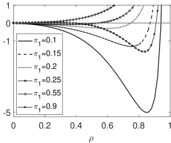
B. Comparison of the extreme cases α = 0 and α = ∞ In Figure 3 we plot function ∆ with respect to ρ for K = 2 servers and several values of π

1

, and π

2

. From Equation (5), we obtain that ∆ < 0 iff π

1

< 0.5. We note that mobility has a bad impact for the case π

1

= 0.1 until loads ρ < 0.9. Here π

1

is such that the delay of a job in the system with no mobility reminds smaller than that of the system with mobility α = ∞.

We also observe that as π

1

→ 0.5, ∆ becomes positive at smaller load values. Additionally, for any π

1

, as ρ → 1, ∆ is positive. This event can be argued in the following way: as ρ → 1 , we expect that | N ~

^∞

| approaches a single server queue with capacity µ, which is more efficient than a ¯ K parallel M/M/1 system with capacities µ.

Another particular event holds when π

₁

= 0.9. We observe that for intermediate values of ρ, the system with no mobility has better performance. This shows that under arbitrary loads, mobility might also have a negative impact on the performance of the system.

VI. C

ONCLUSIONS

The main takeaway message of this paper is that mobility might not always have a positive impact on the performance of the system even if it improves its throughput. This result was not evident at first, since there are several recent papers where the opposite conclusion had been reached. Due to the complexity of analysis, we have restricted the performance analysis to low loads, i.e., the so-called light traffic regime.

Our analysis shows that mobility need not always improve

the performance, and we have characterized a condition such

that, if satisfied, the performance might improve or deteriorate

as mobility increases. Numerical solutions of the stationary

distribution show that under moderate loads, mobility might

(6)

Mean number of jobs with respect to α for different loads ρ

0 10 20 30

1.9 2 2.1

2.2 10^-3

= 0.001

0 10 20 30

0.0195 0.02 0.0205 0.021 0.0215 0.022

= 0.01

0 10 20 30

0.2 0.21 0.22 0.23 0.24

= 0.1

0 10 20 30

0.55 0.6 0.65 0.7

= 0.25

0 10 20 30

1.5 1.6 1.7 1.8 1.9 2

= 0.5

0 10 20 30

4 4.5 5 5.5 6

= 0.75

Fig. 1. Mean number of jobs depending onαforK= 2and from left to right an increasing set of load values. For fixed parametersµ1= 1.5,µ2= 1, p1= 0.6,p2= 0.4,r12= 0.5. The black filled line corresponds to the system withr21= 0.2and the dashed line to the one withr21= 0.7.

0 2 4 6 8

8.1 8.2 8.3 8.4 8.5

10 ^-4

R

1

R

2

R

3

Fig. 2. E(|N~^α|) for K = 3 servers. Fixed parameters pi = 1/3 for i = 1,2,3 and µ1 = 1, µ2 = 1.2 and µ3 = 1.5. Three different system with R^α₁ = {r₁₂ = 0.7129, r13 = 0.9783, r21 = 0.4348, r23 = 0.0772, r13 = 0.0779, r23 = 0.6541}, R^α₂ = {0.1566,0.9730,0.0412,0.1029,0.1653,0.9898} and R^α₃ = {0.0461,0.4632,0.3701,0.0722,0.5812,0.0773}.

have a negative effect on the performance of the system.

However, under high loads we observe that mobility does improve the performance and the system with α = ∞ has the minimum delay.

0 0.2 0.4 0.6 0.8 1

-5 -1 0 1

1

=0.1

1

=0.15

1

=0.2

1

=0.25

1

=0.55

1

=0.9

Fig. 3. ∆(λ) = E(|N~⁰|)−E(|N~^∞|) for K = 2 servers. For fixed parametersµ1 = 1.5> µ2= 1,p1 = 0.6,p2= 0.4andπ1, π2 ∈(0,1) such thatπ1+π2= 1.

R

EFERENCES

[1] M. Grossglauser and D. N. C. Tse, “Mobility increases the capacity of ad hoc wireless networks,”IEEE/ACM TRANSACTIONS ON NETWORK- ING, VOL. 10, NO. 4, August 2002.

[2] T. Bonald, S. Borst, N. Hegde, M. Jonckheere, and A. Proutiere, “Flow- level performance and capacity of wireless networks with user mobility,”

Queueing Syst (2009) 63: 131–164, 2009.

[3] S. Borst and F. Simatos, “A stochastic network with mobile users in heavy traffic,”Queueing Syst., vol. 74, no. 1, pp. 1–40, 2013.

(7)

[4] T. Bonald, S. Borst, and A. Proutiere, “How mobility impacts the flow- level performance of wireless data systems,” Proc. INFOCOM ’04,, vol. 4, pp. 1872–1881, Mar. 2004.

[5] F. Simatos and D. Tibi, “Spatial homogenization in a stochastic network with mobility,”Ann. Appl. Probab., vol. 20, no. 1, pp. 312–355, 2010.

[6] A. Ganesh, S. Lilienthal, D. Manjunath, A. Proutiere, and F. Simatos,

“Load balancing via random local search in closed and open systems,”

Queueing Syst (2012) 71:321–345, no. 71, p. 321–345, 2012.

[7] J. Walrand, “Chapter 11 queueing networks,” inStochastic Models, ser.

Handbooks in Operations Research and Management Science, D. Hey- man and M. Sobel, Eds. Elsevier, 1990, vol. 2, pp. 519 – 603.

[8] D. Gamarnik and A. Zeevi, “Validity of heavy traffic steady-state ap- proximations in generalized jackson networks,”The Annals of Applied Probability 2006, Vol. 16, No. 1, 56–90, 2006.

[9] P. Robert,Stochastic Networks and Queues. Springer-Verlag, 2003.

A

PPENDIX

A. Proof of Proposition 4.2

By definition of geometric Lyapunov functions, see [8], we need to fix mobility speed α

^∗

, initial state ~ n

^∗

and parameters t

^∗

, η such that

E

_~_n^α

h

e (

θ|N~^α(t^∗)|

) i

e

^θ|^N^~^α^(0)|

< 1 − η (8)

∀| N ~

^α

(0)| = |~ n

^α

| ≥ |~ n

^∗

| and α ≥ α∗. We develop Equation (8) in order to obtain the bound:

E

_~_n^α

h

e (

θ|N~^α(t)|

) i e

^θ|^N^~^α^(0)|

= E

_~^α_n

h

e (

^θ

(

|N~^α(0)|+A(t)−PK i=1

Rt

0D_i(du)1(N_i^α(u⁻)>0)

)) i e

^θ|^N^~^α^(0)|

= E

_~_n^α

h

e (

^θ

(

A(t)−PK i=1

Rt

0D_i(du)1(N_i^α(u⁻)>0)

)) i

(9) where A(t) denotes the total number of arrivals to the system at time t and D

_i

(t) is the number of potential departures at server i at time t for i = 1, . . . , K.

We denote by N ~

_c^α

(t) the closed system where only the N ~

^α

(0) initial jobs are present and has mobility speed α. Thus, for all t > 0, | N ~

^α

(t) − N ~

_c^α

(t)| ≤ A(t) + P

K

i=1

D

i

(t) = ξ and (9) is bounded by the following,

E

_~_n^α

h

e (

^θ

(

A(t)−PK i=1

R_t

0D_i(du)1(N_i^α(u⁻)>0)

)) i

≤ E

_~_n^α

h

e (

^θ

(

^A(t)−^P^Ki=1

Rt

0Di(du)1(N_c,i^α(u)>ξ)

)) i (10) We divide the value space of ξ in two disjoint subsets: (ξ ≥

√ n

^∗

) and (ξ < √

n

^∗

). Therefore, (10) equals

E

_~_n^α

h

e (

^θ

(

A(t)−PK i=1

Rt

0D_i(du)1(N_c,i^α(u)>ξ)

)) i

= E

_~^α_n

h

e (

^θ

(

^A(t)−^P^Ki=1

Rt

)); ξ ≥ √ n

^∗

i

(11) +E

_~_n^α

h

e (

^θ

(

^A(t)−^P^Ki=1

Rt

)); ξ < √ n

^∗

i

(12)

In the following we analyse each expressions on its own.

For Equation (11), notice that ξ = A(t) + P

K

i=1

D

i

(t) is distributed by a Poisson process of rate (λ + ¯ µ)t.

E

_~_n^α

h

e (

^θ

(

^A(t)−^P^Ki=1

Rt

)); ξ ≥ √ n

^∗

i

≤ E

_~_n^α

"

e

^θA(t)

; ξ = A(t) +

K

X

i=1

D

i

(t) ≥ √ n

^∗

#

≤ E

_~_n^α

h

e

^θξ

; ξ ≥ √ n

^∗

i

= f

_θ,t

( √

n

^∗

) < η

2 (13)

Then, as √

n

^∗

→ ∞, f

_θ,t

( √

n

^∗

) → 0. Therefore, there exists a constant value, say

^η₂

that bounds Equation (11).

On the other hand, turn back attention to Equation (12).

Now we develop the second term of the sum, E

_~_n^α

h

e (

^θ

(

^A(t)−^P^Ki=1

Rt

)); ξ < √ n

^∗

i

= E

_~_n¹

h

e (

^θ

(

A(t)−PK i=1

Rt

0D_i(du)1(N_c,i(αu)>ξ)

)); ξ < √ n

^∗

i (14)

≤ E

_~_n¹

h

e (

^θ

(

^A(t)−^P^K_i=1^R₀^t^Di(du)1(N_c,i(αu)>√ n^∗)

)) i

(15) For equality (14), we rescale the system in the following way: (N

_c^α

(t), t ≥ 0) with mobility transition rate matrix αR is equivalent to (N

_c¹

(αt), t ≥ 0) with transition rate matrix R. We remove superscript 1 from now on.

Now, we focus on the initial state ~ n and fix it as the one with maximum expected value, ~ n

_m

. This further implies that the maximum is obtained for some initial state such that |~ n

_m

| ≥

|~ n

^∗

|. However, the maximum is obtained at |~ n

m

| = |~ n

^∗

| by applying the following argument consecutively. Denoted by N ~

_c^~ⁿ^m

a closed system with |~ n

m

| particles that starts at position

~ n

^m

. Thus, 1(N

_c,i^~ⁿ^m

(t) > √

n

^∗

) ≤ 1(N

_c,i^~ⁿ^m^+eⁱ

(t) > √ n

^∗

) for any t. This happens until the least number of particles given by |~ n

m

| = |~ n

^∗

|. Therefore, take

~

n

m

∈ arg max

~n:|~nm|=|~n^∗|

n E

_~_n

h

e (

^θ

(

^A(t)−^P^Ki=1

Rt

0Di(du)1(Nc,i(αu)>√ n^∗)

)) io Remark that ~ n

m

depends on variables α and t, which will be lately fixed. Thus, ~ n

m

= ~ n

m

(α, t). Once ~ n

m

is fixed, we look at closed system N ~

^m

(t), which starts at position ~ n

m

and has |~ n

m

| = |~ n

^∗

| particles. Therefore, (15) is upper bounded by the followings:

E

_~_n

h

e (

^θ

(

^A(t)−^P^Ki=1

Rt

0Di(du)1(Nc,i(αu)>√ n^∗)

)) i

≤ E

~n_m

h

e (

^θ

(

A(t)−PK i=1

Rt

0D_i(du)1(N_c,i^m(αu)>√ n^∗)

)) i

= e

^λt(e^θ⁻¹⁾

E

_~_n_m

"

_K

Y

i=1

e (

^−θ^R₀^t^Di(du)1(N_c,i^m(αu)>√ n^∗)

)

#

= E

~n_m

h

e (

^λt(e^θ⁻¹⁾⁻^P^Ki=1µi(1−e^−θ)Rt

01(N_c,i^m(αu)>√ n^∗)du

) i

(16)

(8)

By applying the Laplace transform of a Poisson process and then verifying that 1 − e

^−θ1(N^c,i^m^(αu)>

√n^∗)

= 1(N

_c,i^m

(αu) >

√ n

^∗

)(1 − e

^−θ

), equality (16) holds.

Denote by Z(α) = P

K

i=1

µ

i1 t

R

t

0

1(N

_c,i^m

(αu) >

√ n

^∗

)du. First, by a change of variables, Z(α) = P

K

i=1

µ

i 1 αt

R

αt

0

1(N

_c,i^m

(u) > √

n

^∗

)du. Take Z

^∗

= inf

_α≥α^∗

Z(α). Then, (16) is bounded by the following:

E

_~_n_m

h

e (

^λt(e^θ⁻¹⁾⁻^P^Ki=1µ_i(1−e^−θ)Rt

01(N_c,i^m(αu)>√ n^∗)du

) i

≤ E

~n_m

h

e (

^λt(e^θ−1)−t(1−e^−θ)Z^∗

) i

(17) From the ergodic theorem, see [9], when α

^∗

→ ∞, Z

^∗

converges almost surely into P

K

i=1

µ

_i

E

_~_n_m

(1(N

_c,i^m

(t) >

√ n

^∗

)) = P

K

i=1

µ

i

P

~n_m

(N

_c,i^m

(t) > √

n

^∗

) in steady-state. Last distribution expression has the shape of a multinomial distribution. Denote P

K

i=1

µ

i

P

~n_m

(N

_c,i^m

(t) > √

n

^∗

) = z

^∗

(n

^∗

, √ n

^∗

).

Additionally, P

x^∗

(N

_c,i^m

(0) > √

n

^∗

) → 1 as n

^∗

→ ∞, for all i = 1, . . . , K. Hence, z

^∗

(n

^∗

, √

n

^∗

) → µ. From the hypothesis: ¯ θ is such that λ(e

^θ

− 1) −

^{λ+ ¯}₂^µ

(1 − e

^−θ

) < 0. Therefore, e

^λ(e^θ^{−1)−(1−e}^−θ^{) ¯}^µ

< e

^(1−e^θ⁾^λ−¯²^µ

.

E

_~_n_m

h

e (

^λt(e^θ^{−1)−t(1−e}^−θ^)Z^∗

) i

= E

~n_m

h

e (

^λt(e^θ−1)−t(1−e^−θ)(Z^∗±z^∗(n^∗,√ n^∗)

) i

= e

^λt(e^θ^{−1)−t(1−e}^−θ^)z^∗⁽ⁿ^∗^,

√n^∗)

×E

_~_n_m

h

e (

^−t(1−e^−θ^)(Z^∗^−z^∗⁽ⁿ^∗^,^√ⁿ^∗⁾

) i

< e

^t(1−e^−θ⁾^λ−¯²^µ

E

_~_n_m

h

e (

−t(1−e^−θ)(Z^∗−z^∗(n^∗,√ n^∗)

) i

(18) Therefore, initial expression (10) is bounded by (13) and (18):

E

_~_n^α

h

e (

^θ

(

^A(t)−^P^Ki=1

Rt

)) i

≤ η

2 + e

^t(1−e^−θ⁾^λ−¯²^µ

E

_~_n_m

h

e (

^−t(1−e^−θ^)(Z^∗^−z^∗⁽ⁿ^∗^,^√ⁿ^∗⁾

) i (19) Fix t = 1. From stability, e

^(1−e^−θ⁾^λ−¯²^µ

is positive and strictly smaller than 1. Say it is bounded by 1 − η, for some small η > 0. Lastly, since stated before, Z