HAL Id: hal-01107720
https://hal.archives-ouvertes.fr/hal-01107720
Submitted on 25 Jan 2015
HAL is a multi-disciplinary open access
archive for the deposit and dissemination of
sci-entific research documents, whether they are
pub-lished or not. The documents may come from
teaching and research institutions in France or
abroad, or from public or private research centers.
L’archive ouverte pluridisciplinaire HAL, est
destinée au dépôt et à la diffusion de documents
scientifiques de niveau recherche, publiés ou non,
émanant des établissements d’enseignement et de
recherche français ou étrangers, des laboratoires
publics ou privés.
Indexing Evidential Data
Anouar Jammali, Mohamed Anis Bach Tobji, Arnaud Martin, Boutheina Ben
Yaghlane
To cite this version:
Anouar Jammali, Mohamed Anis Bach Tobji, Arnaud Martin, Boutheina Ben Yaghlane. Indexing
Evidential Data. Third World Conference on Complex Systems, Nov 2014, Marrakech, Morocco.
�hal-01107720�
Indexing Evidential Data
Anouar Jammali
∗, Mohamed Anis Bach Tobji
†, Arnaud Martin
‡and Boutheina Ben Yaghlane
§∗LARODEC, University of Tunis, ISG, Tunisia
Email: [email protected]
†LARODEC, University of Manouba, ESEN, Tunisia
Email: [email protected]
‡IRISA, University of Rennes 1, IUT of Lannion, France
Email: [email protected]
§LARODEC, University of Carthage, IHEC, Tunisia
Email: [email protected]
Abstract—Querying imperfect data received increasing at-tention in the area of database management. The complexity and the volume of imperfect data requires advanced techniques for efficient access, and satisfying user-queries in a reasonable response time. In this paper, we are particularly interested in evidential databases, i.e., databases where imperfection is represented through Dempster-Shafer theory. To answer user-queries in such databases, we propose a new index system based on a tree data structure (e-Tree) that is adapted to the complexity of the evidential data. The experiments done on our solution showed encouraging results.
Keywords—Dempster-Shafer theory, indexing data, evidential database.
I. INTRODUCTION
Imperfect databases research field is receiving a quite important attention from academic and industrial researchers in the recent years. That is due to the need of database manage-ment systems (DBMS) that handle different data natures and support decision making process in presence of uncertainty.
Several real world applications suffer from data imper-fection. For example, in medical applications, symptoms and diagnosis data are infected with imperfection (be it uncertainty, incompleteness or imprecision). Also, data collected from sensors deal with imperfections. The sensors of a unique system may have different precision levels, thus, the system that manages these data should be as robust as possible to correctly cope with data imperfection.
In this work, we are interested in imperfect data that are modeled through Dempster-Shafer theory [9], [10], [15] called,
evidential data. Evidential database is the system that stores and manages evidential data, with regarding to its complex nature. Handling uncertainty and imprecision via evidential database systems is an active research topic tackled in several works such as [6], [7], [12], [4].
When we deal with huge volume of data [5], the cost of accessing these data becomes problematic. A trivial solution to minimize this cost is to use an indexing system. However, conventional indexes used in traditional (perfect) databases are unusable in evidential databases, because non adapted to the structure of the evidential data. Even index structures introduced in the uncertainty context, cope with probabilistic databases [16], [11], [2], [13] rather than with evidential ones.
In this work, we introduce a new tree based data structure as an indexing system adapted to the nature of data stored in evidential databases. The introduced structure is a single attribute index, i.e., an index based on a unique database column. To validate our contribution, we implemented the sequential access to the evidential database, which is the trivial solution to answer user-queries, the Rid Lists structure, introduced in [3] and adapted in this paper to index evidential data, and finally the evidential tree, called e-Tree, introduced in this article. Then we led experiments on these methods to compare their efficiencies for various synthetic evidential databases.
This paper is organized as follows:
In section 2, we present the background material of our work. In subsection A, the basic notions of Dempster-Shafer theory are introduced, to present then, in subsection B, the evidential database concept which is based on the aforementioned the-ory. In section 3, we present the indexes of evidential data. Two solutions are presented; the RID Lists structure, initially proposed in [3] for mining association rules, and the e-Tree structure that is the contribution of this work. Finally, in section 4, we present the experiments conducted on our index systems as well as the obtained results.
II. BACKGROUNDMATERIAL
A. Dempster-Shafer (DS) Theory
A discernment frame is a set of mutually exclusive and exhaustive hypotheses where one of these hypotheses is likely to be the solution for the proposed problem. The uncertain information representation can be expressed by the mass function:
Let Ω be a frame of discernment, then, a function m : 2Ω→ [0, 1] is called a mass function whenever:
m(∅) = 0 X
A⊆Ω
m(A) = 1 (1)
An element A of the set 2Ω
is called a focal element whenever m(A) 6= 0. The measure m(A) gives how much is true the hypothesis A.
From this definition are derived the definitions of belief (bel) and plausibility (pl).
The belief value of an attribute A, denoted by bel(A), is the total mass of all subsets of A. It reflects the total belief committed toA. belΩ: 2Ω→ [0, 1] belΩ(A) = X B⊆A mΩ(B) (2)
The plausibility function is the dual function of belief. It measures the maximum amount of belief that could be given to a propositionA.
This function gives how much the given information enforces the hypothesis A. It is defined on 2Ω
→ [0, 1] as follows: plΩ(A) = 1 − belΩ( ¯A) plΩ(A) = X B∩A6=∅ mΩ(B) (3)
where ¯A is the complement hypothesis of A.
B. Evidential Database
An evidential database EDB is a database with X at-tributes andY lines where each attribute Ax(1 ≤ x ≤ X) has a domainΩxcontaining all the possible hypotheses, i.e., values ofAx.Ωxis the frame of discernment of thexthattribute. The value of the jthattribute in theithline is called an evidential
value denoted by Vij. An evidential value is a basic belief
assignment (bba) defined through a mass function denoted by mij.
Table 1 is an example of an evidential database, where the attribute Disease stores the diagnosis of a patient. The diagnosis of a patient may be precise and certain, as the diagnosis of John. It may be uncertain, like the diagnosis of Robert. Also, it may be imprecise, like for the patient Maria. This evidential attribute may contain any imperfect information that could be modeled through the DS theory.
Table I. Diagnosis: ANEXAMPLE OFEVIDENTIALDATABASE
Id Patient Disease
1 Robert 0.7 flu, 0.3 anemia
2 Celina 0.7 (cancer,flu), 0.3 cancer
3 John flu
4 Maria (anemia,cancer)
In [14], the author introduced an interesting model of an extended relational evidential database. The main contribution of this work is a generalized relational algebra where five rela-tional operators (projection, restriction, cross product, intersect and join) are redefined.
In this paper, we are content with giving a simple example of selection from one table. For more details, please refer to the articles [14] and [6].
Assume we want to evaluate the following query:
SELECT * FROM diagnosis WHERE disease=’flu’
In a perfect database, the result of this query contains every line whose attribute Diagnosis has the value flu. In
evidential databases, attributes contain evidential values rather than precise values. Thus, the result contains the lines where belief of flu is strictly positive in the bba of the Diagnosis attribute(bel(f lu) > 0). It is formally defined as follows:
tab<attribute=v>= {l ∈ edb/bell(v) > 0} (4) where tab<attribute=v> is the restriction of the relation tab according to conditionattribute = v, and bell(v) is the belief of v in the record l.
Note the pseudo-attributeBel added to the resulted relation (see Table 2). It represents the belief of the searched value (in our example flu) in the resulted line.
In [14], the resulted lines are those where pl(flu) is strictly positive (pl(f lu) > 0). A pseudo-attribute called Confidence
Level (denoted by CL) is added to the returned relation. It is an interval delimited by the belief and the plausibility of each resulted line as shown in table 3.
Table II. Diagnosis<disease=′f lu′>
Patient Disease Bel
Robert 0.7 flu, 0.3 anemia 0.7
John flu 1
Table III. Diagnosis<disease=′f lu′>ACCORDING TO MODEL OF[14]
Patient Disease CL
Robert 0.7 flu, 0.3 anemia [0.7,0.7] Celina 0.7(cancer,flu), 0.3 cancer [0,0.7]
John flu [1,1]
Thus, in the literature, there are two models for answering user-queries in evidential databases. In the first one, we return lines where believes of the searched value are positive. In the second model, returned lines are those whose plausibilities of the searched value are positive. In this paper, we focus only on the first model.
III. INDEXINGEVIDENTIALDATABASES
Answering a query of the formtable < attribute = V > leads to computing the belief of the searched value (V ) in each line of the database. The DBMS has not only to look for the searched value, but also for the subsets of the searched value (see the definition of the belief function in section 2, subsection A). For example, assume that the searched value is V = {cancer, f lu}. The DBMS should find all lines that deal with {cancer, f lu}, but also with cancer and f lu values. If the searched value V has a size n, then the DBMS must return each line that deals with any subset A ⊆ V from the 2n possible focal elements in the database that are subsets ofV . Thus, answering queries in evidential databases is much more costly than answering queries in perfect databases. Consequently, it is obvious that efficient query processing techniques are needed. Indexing remains a key technique to this aim.
In this section, we will present two indexing techniques. The first one is derived from the work [3], where RID Lists are used to mine frequent itemsets in evidential data. And the second one is introduced in this paper. It is a tree data structure that represents evidential data in a manner that accelerate the search operation.
A. The RID Lists structure
The RID Lists structure assigns to each focal element in the indexed attribute a list of couples. Each couple that concerns a focal element f e contains two information:
• The row identifier (ROWID) of the line that contains f e.
• The mass off e in that line.
The RID Lists corresponding to the diseases’ database (table 1) is presented in table 4. The construction algorithm of the RID Lists structure, corresponding to an evidential database, is detailed in [3].
To evaluate the query table<attribute=v>, the RID Lists index is scanned, and every RID List related to a focal element included in v, is returned. To accelerate the search, the RID Lists is sorted in the construction phase.
Table IV. RIDLISTS OF TABLEDiagnosis
Focal element Rid List
anemia (1,0.3)
{anemia,cancer} (4,1.0)
cancer (2,0.3)
{cancer,flu} (2,1.0)
flu (1,0.7)(3,1.0)
B. The Evidential Tree
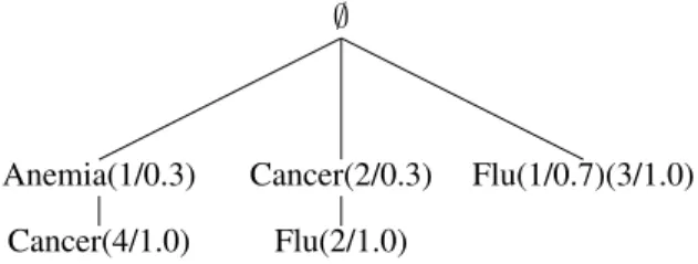
The evidential tree, denoted by e-Tree, is a tree data structure that stores the content of an evidential attribute A. The root of the tree is the empty set. A node of the tree has two information:
• A value x ∈ DA where DA is the domain of the attributeA.
• A list of couples (rid,bel).
Each couple (rid, bel) informs about the belief of the focal element f e in the line whose identifier is rid. f e is the focal element that is composed of values ofA in the path that starts from the root, to the current node.
For example, in figure 1, see the nodecancer(4/1.0). It means that the focal element {anemia, cancer} (see the path that starts from the root and ends in the cancer node) has a belief equal to 1.0 in the line 4.
Note that e-Tree is sorted in breadth and in depth. It allows us to accelerate the search operation. In the following, we present two important algorithms. The first one is about the construction of the e-Tree from an evidential database. The second one deals with searching lines that cope with a search value, from an e-Tree structure.
1) Construction of the e-Tree: The construction of e-Tree is described in the pseudo-code of the algorithm 1. In each line of the database, each focal element is inserted in depth into the e-Tree. For example, to insert focal elements of the line 2 in the database example (table 1), we begin by the element {cancer, f lu}. We look among the children of the root if there is a node relative to the value cancer. If we don’t find it, we create a node with the label cancer. Then, we look among the children of this node for a node labeled
f lu. If its exists, we update its RID Lists by adding the couple (2, 1.0), and not the couple (2, 0.7) since belief of {cancer, f lu} in the line 4 is equal to 1 (bel({cancer, f lu}) = mass({cancer, f lu}) + mass(cancer) = 1).
Then, we handle the second focal element in line 2, that is cancer. We look for the node cancer in children’s root, and we find it (it is just created). So we add the couple (2, 0.3) to its RID Lists. Algorithm 1 presents the pseudo-code of constructing the evidential tree from an evidential database. Figure 1 illustrates the evidential tree corresponding to the table Diagnosis. ∅ Anemia(1/0.3) Cancer(4/1.0) Cancer(2/0.3) Flu(2/1.0) Flu(1/0.7)(3/1.0)
Figure 1. e-Tree corresponding to the table Disease
2) Searching in the e-Tree: A user query may cope with a precise or imprecise value. For example, a user may search for lines with a precise diagnosis, such as flu. He also may look for lines with imprecise diagnosis, like{anemia, cancer}. If the searched value is precise, then e-Tree structure is scanned only at its first level. The other levels are about imprecise values, i.e., compound focal elements. That is an advantage relatively to the RID Lists structure, where singleton focal elements are not collected in a separate structure. In the e-Tree structure, singleton focal elements are stored as the children of the root node. If the searched value is precise, the search algorithm scans only n elements, while in the RID Lists, it scans up to2n elements. In this case, we can apply dichotomic search since nodes are sorted. Consequently, the complexity of the search algorithm islog2(n).
When the searched value V is imprecise, like {anemia, cancer}, the search algorithm looks for nodes that correspond to anemia and cancer in the first level. It also looks for the nodes that represent the focal element {anemia, cancer} which is at the second level. To make faster, when the searched value V is imprecise, each time we visit a node relative to an element e belonging to V , a depth-scan is performed to look for all children of e that are included (subsets) in V . In our example, when we visit the node anemia, we also scan its children, looking for the node cancer. This node, that represents the focal element {anemia, cancer} is also concerned by the search operation. The search algorithm returns the line 1 (with the belief 0.3), and then returns the line 4 (with the belief 1). Depth searching linked with the singleton anemia being complete, the search algorithm go to the next singleton element of V , that is cancer. The same recursive operation done for the node anemia is done for cancer.
A main advantage of e-Tree relatively to the RID Lists index, is that the hypotheses composing the focal elements are linked. Exploring a singleton value, leads directly to all nodes it prefixes, and that are subsets inV . In the RID Lists structure, subsets ofV are separated, which necessitates more scan time.
Algorithm 2 is the general method to search a value V in an e-Tree structure. The output is a set of lines (identified by a rid) with the belief of V in each one (like in table 2). Algorithm 3 is the procedure used recursively in the main algorithm. The procedure SEARCH takes as input a node N in e-Tree, The searched value V and k as the level where the search will perform. It adds to the set of returned lines the couples of(rid, bel) that satisfy the search criterion in the levelk. Note that in algorithms 1, 2 and 3, N.children[] is the set of the nodes that are children of the nodeN ; subsets(V, k) is the collection of all subsets of V whose sizes are equal to k; P AT H(c) returns the focal element that is composed of all nodes’ elements that link the root node to the node c.
Algorithm 1: Construction of e-Tree
input : An evidential table edb output: e-Tree
for each line l in edb do
for each focal element f e in l do if f e is singleton then
if f e ∈ root.children[] then Update the RID List of f e; else
Add a node for f e;
Initialize Its RID List with the couple(ridl, bell(f e));
end
else /* f e is not a singleton */
for each value v in f e do
scan e-Tree in depth to find the node corresponding to v;
if v not found then
Create a node relative to v in the corresponding level
end end
Add the couple(ridl, bell(f e)) to the leaf
corresponding to f e ; /* It corresponds to the last node visited for the last v in f e */
end end end
Algorithm 2: Searching a valueV in e-Tree
input : e-Tree, V as the searched value
output: returned lines as a set of couples(rid, bel) for each child c in root.children[] do
if c in subsets(V ,1) then
ADD c.ridlists TO returned lines; SEARCH(c, V,2, returned lines); end
end
IV. EXPERIMENTS ANDRESULTS
A. Generation of evidential databases
We present in this section the experiments made on several synthetic evidential databases, in order to show the behavior of our indexes when processing user queries on scalable evidential data. Evidential databases are not abundant in real world, thus, we generated synthetic data. We implemented a
Algorithm 3: The procedureSEARCH
input : N as a node in e-Tree, V as the searched value, k as the searched level
output: returned lines as a set of couples(rid, bel) for each child c in N.children[] do
if PATH(c) in subsets(V ,k) then
ADD c.ridlists TO returned lines; SEARCH(c, V, k+ 1, returned lines); end
end
generator program that produces a database with only one attribute. We recall that our indexes are single attribute based, i.e., indexes based on a unique attribute, so we do not need to databases with several attributes. The generation takes into account several parameters that cope with the evidential database nature.
The parameterD is the size of the database. It provides the number of lines in the database. The parameterN F E is about maximum number of focal elements in one bba. For example, in the database of table 1, N F E is equal to 2, since the maximum number of focal elements per line is 2 (see lines 1 and2). The parameter SF E is the maximum size of compound focal element. In our database example,SF E is also equal to 2 (see lines 2 and 4 that include composed focal elements). The parameter CARD is the cardinality of the indexed attribute. It is the size of the frame of discernment. In our example, we have CARD = 3 because the diagnosis attribute has three possible values: anemia, cancer and flu. Finally, the parameter P CT IM P is about the rate of imperfect lines in the database. It is the ratio (number of imperfect lines ×100)/(D). In our example, P CT IM P = 75%.
The generation program produces exactlyD lines. In each one, it generates n focal elements, where n is chosen in the interval [1, N F E]. Then, for each focal element, it chooses a value s ∈ [1, SF E], that is the size of the focal element. Thus, content of a focal element is composed ofs hypotheses. Each one is generated such that valuev of one element is taken from the interval[1, CARD]. Finally the masses of the n focal elements are chosen each one in the interval [0, 1] under the condition Pni=1m(v) = 1. Values of n, s and v are computed in their respective intervals through the uniform law.
B. Evaluating the access methods
We created several synthetic databases with various val-ues of the parameters above, and we implemented three access methods to evidential databases. The first access to the database uses the e-Tree index, the second one uses the RID Lists index, and the third one do not use any index system.
In the first experiment, we set the parametersN F E, SF E, CARD and P CT IM P respectively to 3, 3, 12 and 75%, and we varied the value of the parameter D from 300 to 1200. The figure 2 shows that performing an access without index is more expensive, in time execution, than an index based search. This expected result is due to the fact that using an index structure avoids scanning the whole of the database. Note that when the size of the database increases, the execution time is exponentially worse for the non-index method. Using indexes is much more efficient when the size of the database increases
considerably. The e-Tree gives better results than the RID Lists index since searched elements are linked. For example, in the RID Lists, if the searched value is{A1, A2, A3}, then we have to find and to visit separately the lists of the focal elementsA1, {A1, A2} and {A1, A2, A3}. With the e-Tree index, reading the path A1 → A2 → A3 is sufficient to obtain the same information, which is composed of the row identifiers of the interesting lines, and also their believes in. This advantage is very clear in the experiment of varying the SF E parameter (see figure 3). In this experiment, we generate several databases where parametersD, N F E, CARD and P CT IM P are set respectively to 1000, 3, 12 and 75% with a variation of SF E from 1 to 3. When SF E is set to 2, using the e-Tree is more efficient than using RID Lists index. When SF E is set to 3, the performance of RID Lists index decreases considerably, contrary to the one of e-Tree that remains practically the same. The difference between the two methods’ efficiencies is more considerable when the size of the indexed focal elements (SF E) increases as explained in the previous example.
Figure 2. Behavior of access methods when D varies
Figure 3. Behavior of access methods when SF E varies
Next experiment deals with the variation of the number of focal elements (N F E) parameter. The results (see figure 4) show same behavior of the three methods. Note here that if the number of focal elements per line increases, the probability that we have several nested focal elements per line also increases. Again, in that case, e-Tree outperforms widely RID Lists as explained in the previous experiment.
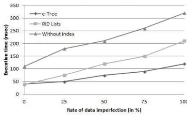
We also generated several databases with various imperfec-tion rates. Values of the parameter P CT IM P were varied from 0% (all data are perfect) to 100% (all lines contain evidential values). The experiment’s results are shown in figure
5. Note in this experiment that e-Tree and RID Lists give the same performance for a null value ofP CT IM P . This result will be interpreted in subsection C.
Figure 4. Behavior of access methods when N F E varies
Figure 5. Behavior of access methods when imperfection rate varies
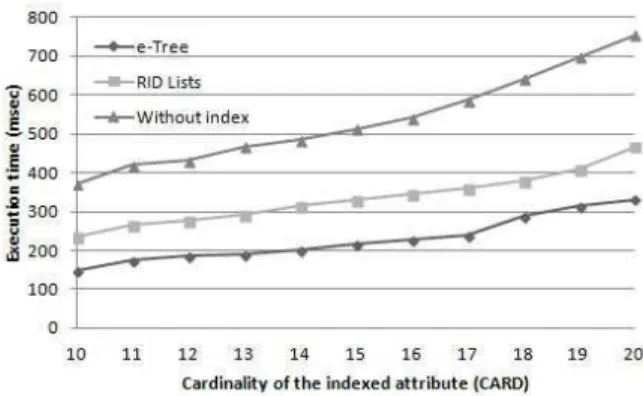
We performed another important experiment on variation of the CARD parameter. D, N F E, SF E, and P CT IM P are set respectively to 1000, 3, 3 and 75%, and the cardinality of the indexed attribute were varied from10 to 20. Note that when the cardinality of the attribute is n, the total number of focal elements may reach2n. So when n is set to 20, the potential number of focal elements in the database is theoretically 220
. Of course, in real situations, focal elements do not include a great number of hypothesis especially when they are expressed by human experts [8]. Thus, setting the maximum size of focal elements to 3 is sufficient to mimic real bbas. In our case, the number of potential focal elements in the whole of the database, when CARD = 20 and SF E = 3 is equal to P3
k=1C20k = 1350. In other words, even though the cardinality of the indexed attribute is equal to 20, being imperfect, the attribute may be affected until 1350 different focal elements rather than 220 = 1048576, i.e., all subsets composed of 1, 2 or3 elements of a total of 20 values. Figure 6 shows the results of the experiment. Again, e-Tree benefits from its condensed representation of compound focal elements.
C. The perfect and the probabilistic cases
In experiment related to the variation of the imperfection rate (figure 5), we mentioned that accessing a perfect database (P CT IM P = 0%) using the e-Tree index, or the RID Lists index gives the same result in term of answer time. When
Figure 6. Behavior of access methods when CARD varies
compound focal elements are absent, then the two structures are identical. In this case, the two structures consist in a collection of RID Lists that store the rid couples of each attribute’s value (that is singleton, with belief equal to one).
Moreover, even when SF E = 1 (see figure 3), for any P CT IM P > 0% and N F E > 1, the two structures have exactly the same behavior. That is, when the indexed attribute hasbbas with exclusively singleton focal elements (SF E = 1), the two index structures are equivalent. Note here that with these parameters the database is probabilistic.
D. Influence of queries’ types
In our experiments, we noted that efficiency of access methods depends on the nature of the user-query. There is an important difference between user-queries with simple condition, and the ones with compound conditions. Query that looks for the valueA3 is much more simple than the one that looks for the valuesA1 orA2orA3. To answer to the second query, we must verify 23
= 6 possible combinations in our index. Consequently, we did an experiment on the behavior of our three methods when performing a simple query, and when performing a more complicated query, i.e., query with a compound condition. In this experiment, the query’s condition involves the search of three values. Table V shows execution time for the three access methods relatively to the two queries. Note that even for the simple query, e-Tree based method is better than the RID Lists one. In fact, when we deal with a simple condition query, the access method scans only the nodes (in the e-Tree) and the lists (in the RID Lists) of the singleton focal elements. Since singleton focal elements are collected only in the first level of the e-Tree, the scan is done on a maximum of CARD nodes. However in the RID Lists index, singleton focal elements are stored with the compound ones, and so search is more costly.
Table V. COMPARISON ACCORDING TO THE NATURE OF USER-QUERIES
Access method Simple condition query Compound condition query
e-Tree 101 msec 167 msec
RID Lists 161 msec 211 msec
Without index 307 msec 332 msec
V. CONCLUSION
In this paper, we introduced a new index data structure, called e-Tree, used to accelerate searching operations in
ev-idential databases. The e-Tree structure stores for each focal element in the database, the identifiers of the records where the belief of the searched value is positive. A construction method, and a search method were defined. The experiments we led to evaluate this solution were promising.
REFERENCES
[1] Agarwal C.C. (2009) Managing and Mining Uncertain Data, Advances in Database Systems, Springer.
[2] Agarwal C.C. ; Cheng S.W. ; Cuhk Y. T. ; Hkust K. Y. (2009) Indexing Uncertain Data, Managing and Mining Uncertain Data, Advances in Database Systems Vol 35, PROD’09, Rhode Island, USA, pp 1-26. [3] Bach Tobji, M.A. ; Ben Yaghlane, B. ; Mellouli, K. (2008) A New
Algorithm for Mining Frequent Itemsets from Evidential Databases, International Conference on Information Processing and Management of Uncertainty in Knowledge-Based Systems, Malaga, Spain, pp 1535-1542.
[4] Bach Tobji, M.A. ; Ben Yaghlane, B. (2011) Extraction des item-sets frequents a partir de donnees evidentielles : application a une base de donnees educationnelles, Revue des Nouvelles Technologies de l’Information, vol RNTI-E-21, pp 211-232.
[5] Bayer R. ; McCreight E. (1972) Organization and Maintenance of Large Ordered Indexes, Acta Informatica, vol 1, pp 173-189.
[6] Bell D.A. ; Guan J. W. ; Lee S.K. (1996) Generalized Union and Project Operations for Pooling Uncertain and Imprecise Information, Data & Knowledge Engineering, Vol 18, Issue 2, pp 89117.
[7] Ben Abdelaziz F. ; Pomerol J.C. ; Telmoudi A. (2002) The Evidential Database Model, IEEE International Conference on Systems, Man and Cybernetics, Yasmine Hammamet, Tunisia, pp 110-113.
[8] Denoeux T. ; Bjanger M.S. (2000) Induction of decision trees from partially classified data using belief functions, IEEE International Con-ference on Systems, Man, and Cybernetics, Nashville, US, pp 2923-2928. [9] Dempster A.P. (1967) Upper and Lower Probability Function in a Context of Uncertainty, Annals of math. statistics, vol 38, pp 325-339. [10] Dempster A.P. (1968) A Generalization of Bayesian Inference, Jour. of
the Royal Statistical Society, vol 30, pp 205-247.
[11] Dong T. ; Xiao C. ; Guo X. ; Ishikawa. Y (2013) Processing Probabilis-tic Range Queries over Gaussian-Based Uncertain Data, International Symposium on Spatial and Temporal Databases, Munich, Germany, pp 410-428.
[12] Hewawasam K. ; Premaratne K. ; Shyu M. L. (2005) Rule Mining and Classification in Imperfect Databases, In International Conference on Information Fusion, Philadelphia, USA, pp 661-668.
[13] Huang Y. (2014) Indexing and querying moving objects with uncertain speed and direction in spatiotemporal databases, Journal of Geographical Systems, vol 16, issue 2, pp 139-160.
[14] Lee S.K. (1992) An Extended Relational Database Model For Uncertain and Imprecise Information, University of Iowa, Iowa City, pp 211-220. [15] Shafer G. (1976) A Mathematical Theory of Evidence, Princeton
Uni-versity Press, Princeton.
[16] Wang Y. ; Li. X ; Li. X ; Wang Y. (2013) A survey of queries over uncertain data, Knowledge and Information Systems Vol 37, Issue 3, pp 485-530.