HAL Id: hal-01644897
https://hal.archives-ouvertes.fr/hal-01644897
Submitted on 19 Feb 2018
HAL is a multi-disciplinary open access
archive for the deposit and dissemination of
sci-entific research documents, whether they are
pub-lished or not. The documents may come from
teaching and research institutions in France or
abroad, or from public or private research centers.
L’archive ouverte pluridisciplinaire HAL, est
destinée au dépôt et à la diffusion de documents
scientifiques de niveau recherche, publiés ou non,
émanant des établissements d’enseignement et de
recherche français ou étrangers, des laboratoires
publics ou privés.
Fire detection - A new approach based on a low cost
CCD camera in the near infrared
Yannick Le Maoult, Thierry Sentenac, Jean-José Orteu, Jean-Paul Arcens
To cite this version:
Yannick Le Maoult, Thierry Sentenac, Jean-José Orteu, Jean-Paul Arcens. Fire detection - A new
approach based on a low cost CCD camera in the near infrared. Process Safety and Environmental
Protection, Elsevier, 2007, 85 (B3), pp.193-206. �10.1205/psep06035�. �hal-01644897�
FIRE DETECTION
A New Approach Based on a Low Cost CCD
Camera in the Near Infrared
Y. Le Maoult!, T. Sentenac, J. J. Orteu and J. P. Arcens
Ecole des Mines d’Albi, Albi Tarn, France.
Abstract: In this paper, we present a new system based on a low-cost CCD camera to detect a fire in the near infrared spectral band. After a brief description of the main features of the camera used in the study and the characteristics related to hot spots detection, we point out the interest of this imaging technique compared to classical thermal sensors used in such applications. After-wards, we discuss the choice of the 750–1100 nm region and then we present the different experimental benches developed to validate our approach. The method focuses on the need of a multi-criteria analysis of the fire phenomenon. After a description of the signature of a fire: energy radiated, spatial and temporal fluctuations, the detection method is explained and preliminary results are given.
Keywords: fire detection; CCD camera; near infrared.
INTRODUCTION
The overall objective of this work is to develop a new and more effective remote control approach for the detection and recognition of fire events and/or person intrusion in ware-houses or industrial buildings. Then, the detection system has to take into account the different signatures of the combustion pro-cess and movements in a given place. In this paper, we present only the problem of fire detection and particularly we address the problem of flame detection and recognition. For that, data in different spectral band and flame criteria were analysed. In our specific context, the fire detection system has to detect a 50 mm hot spot at 10 m for a detection time less than 3 s and must provide access to visual inspection on a monitor.
Literature Review
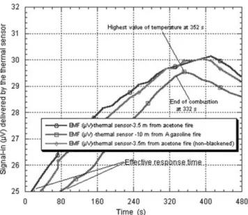
The detection of fires in warehouses or industrial buildings is generally performed with point-based thermal sensors responding to the heat flux emitted by the flames such as thermistors or thermocouples. Therefore, to obtain a realistic spatial coverage of a scene, the number of sensors must be import-ant. On the other hand, effective response time due to the distance between the sensors and the phenomenon is often too long, to ensure a good protection of merchandises stocked in warehouses. As an example, we
show in Figure 1 a typical thermal sensor response that we have recorded inside a specific insulated cell test whose size was very close to one of a little workshop or lab-oratory. The fire source was produced by organic compounds such as acetone or gasoline poured inside a circular pan (100 mm in diameter) disposed at 3.5 or 10 m from the thermal sensor, here a black-ened K thermocouple.
The response times obtained in this experi-ment were in the range (20–80 seconds), with a mean effective response time of 45 seconds. This last value highlights the weakness of this kind of system for both tem-poral as well as spatial aspects (localization) of the phenomena.
Then to improve this point, low-cost infrared sensors with very short response times were introduced, because sophisticated systems such as IR cameras are expensive and fragile and are more dedicated to research works in laboratory as shown in Bedat et al. (1990) and Hayakasa (1996).
In the infrared spectrum, hydrocarbon flames are described by a typical set of well known emission bands. Figure 2(a) presents a line-by-line computation done in our labora-tory of the infrared spectrum of a classical premixed propane–air between the wave-length 2 and 10 mm. The ‘flame’ was assumed to be a one-dimensional slab of iso-thermal mixture composed of combustion gases (CO2and H2O) at 1800 K. Figure 2(b)
!Correspondence to: Dr Le Maoult, Ecole des Mines d’ Albi, Cromep, Campus Jarlard Route de teillet, Albi Tarn, 81013 cedex 09, France.
E-mail: yannick.lemaoult@en stimac.fr
introduced the effect of the path length of cold air (300 K) between the sensor and the hot gases on the infrared signa-ture of the flame.
The luminance, here, is given in arbitrary units. As a result, the 3–5 mm spectral range can be used for fire detec-tion due to the strength of the 4.3 mm CO2band as well as the 1–3 mm spectral range (H2O and CO2 bands). A more relevant approach could be an IR multi spectral system which can be less sensitive to artefacts (non fire sources). As a suggestion, a non exhaustive list of detection criteria could be:
. energy threshold on a single spectral band or on several ones;
. ratio of energy for two different spectral bands: the typical infrared signatures of a fire.
As fire is also a dynamic phenomenon, a temporal criterion can be added:
. the flickering analysis of energy in a spectral band due to the ‘puffing’ frequency of the fire.
A combination of these different criteria can be also per-formed to avoid detection of other sources. Returning to Figure 2(b), a variable length of cold air, between 2–100 m, introduces a significant difference between the real signature of the hot gases (cold path closed to 2 m) and the same sig-nature disturbed by a long optical path. For great distances, Energy ratio for two spectral bands can be highly modified. Then the detection can be irrelevant if the choice of the detection bands is made on a reference spectrum at short distance. To face this problem and to improve the effective-ness of the Multi IR approach, additional UV bands can be introduced in the analysis to ‘confirm’ the detection (UV-Multi IR detection). For the UV detection, the solar blind UV band between 240–280 nm is generally used because in this particular spectral band, no solar radiation can reach a detector settled on the surface of the earth: all the energy in this spectral region has been absorbed by the upper layer of the atmosphere (ozone layer), so the detection is not perturbed by the solar radiation.
Actually, fire detection is made on industrial sites where numerous non fire sources exist such as arc lamps, electrical discharges, and so on. These sources emit important level of energy in the UV blind solar band and so this new problem focuses on the great difficulty to be completely insensitive to non fire sources. All these aspects are well reported in the literature, as we will see later on, where point-based sen-sors are described as well as more recent approaches invol-ving CCD camera which introduced the ability to extract morphological features from digital image processing that is very promising for fire discrimination. Therefore, we have done a literature survey on these key points that can be classified in two main categories:
1) A point-based sensor approach which is chosen in Pfis-ter (1997) and Lloyd et al. (1998). PfisPfis-ter (1997) describes a multi-optical sensors/multi-criteria using the light diffusion phenomenon mixed with thermal detectors distributed in the cell to be monitored. The criteria implemented for the detec-tion of fire are:
. energy level of the phenomenon (energy threshold); . evolution of its temporal gradient;
. the amplitude of fluctuation around a mean energy level.
Figure 2. (a) IR spectrum of a typical premixed propane air flame. (b) Effect of the cold path on the 4.3 mm CO2emission band.
The parameters are analysed, here, with a computer which adjusts the different thresholds with a fuzzy logic method but the reliability is directly related to the number of sensors implemented in the cell. This number can be very important for large enclosures. In Lloyd et al. (1998), a sensor operates at 900 nm (near infrared) and the analysis of fire events is made with a FPD method (fluctuation of a probability density function). To be more complete, an indirect fire detection method by reflection on a wall (hidden fire) is also implemented but only non-fire sources such as constant incandescence lamps are treated.
2) A video-camera-based approach which is described, for example, in Plumbs and Richards (1996) by using an indirect detection method for hidden fires with a mesh of markers of liquid crystals applied on the different walls of a test enclo-sure. These markers are observed with a black and white video camera. The method of identification and localization of the fire are based on analysis of the energy radiated on the film with inverse computations. This method needs exter-nal markers and as for Pfister (1997), the spatial resolution is limited by the number of markers.
Goedeke (1995) describes a detection system based on a colour video camera used for both spatial and temporal analysis of the phenomenon, the video unit is ‘confirmed’ with UV and IR point based sensors for the energy aspects. These last devices perform an accurate analysis of the fire signature that can be insensitive to non-fire sources (sun, lamps). The flickering mode of the energy is also tested and when a real fire signature is detected, the monitoring of the phenomenon is made with the video camera and its evol-ution by an image difference technique. This last method improved drastically the spatial resolution of the detection system but needs additional sensors to confirm the fire detec-tion. At last, Phillips et al. (2000) deals with a method using also a colour video camera: by creating LUT for fire pixels, then by using an image difference technique, non fire sources such as sun are rejected because sun has very low temporal variations, a specific correction is implemented to take into account the effect of the movement of the camera on the effectiveness of the analysis of the scene. The reflections of the fire on a wall or on the ground are also eliminated with the help of a threshold on the area of the phenomenon detected by the camera and with erosion algorithm used to ‘erase’ non connected ‘fire’ pixels. This system is attractive by the computation done on sequences of images and it is able to recognize non-fire sources at 30 frames per second, but unfortunately it cannot detect hot spots if no energy is radiated in the visible part of the optical spectrum. To conclude this short introduction on the state of the art and on the main problems to solve, we have also to keep in mind that atmospheric transmission can play a critical role in the final result of the detection if the choice of spectral bands is not well matched on the specific situation of remote control. A realistic analysis of the infrared fire signature is also a difficult task with simple low cost detector but we saw that a multi-criteria detection such as flame flickering coupled with energy variation is a key parameter to be suc-cessful in a wide set of situations. In most of the cases pre-sented, only point-based sensors were used with limitations on spatial resolution. For video approaches, visible part of the optical spectrum was used for the detection of fire but unfortunately these systems cannot detect hot spots if no
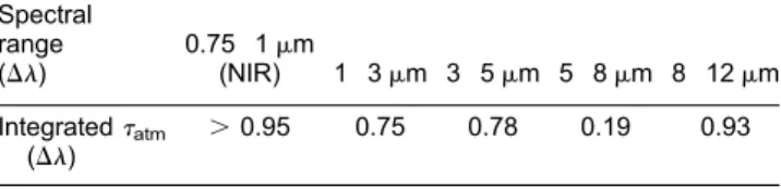
visible radiations are present. Then to complete the approaches of the precedent section, we propose in this study to investigate the problem of fire detection and recog-nition with an uncooled low-cost CCD camera operating in near infrared or NIR (using a near infrared blocking filter). This technique shows, a priori, an interesting potentiality to perform hot spots detection, as precursors of a fire, using thermal imaging in the NIR and then will tend to increase the security of industrial sites by early detection of a blaze. This imaging system gets also the ability to do fire recognition as in the visible spectral range. At last, the NIR spectral range is less affected by atmospheric effects than the other infrared spectral ranges as shown in Table 1.
The computation of atmospheric transmissions (Table 1) use the same line-by-line method and the same conditions as for Figure 2(b): the integrated transmission is computed for a cold path of 100 m, but the hot source is assumed to be here a blackbody at 1500 K, close to a classical mean flame temperature.
MAIN FEATURES OF THE SYSTEM USED FOR THE HOT SPOTS DETECTION
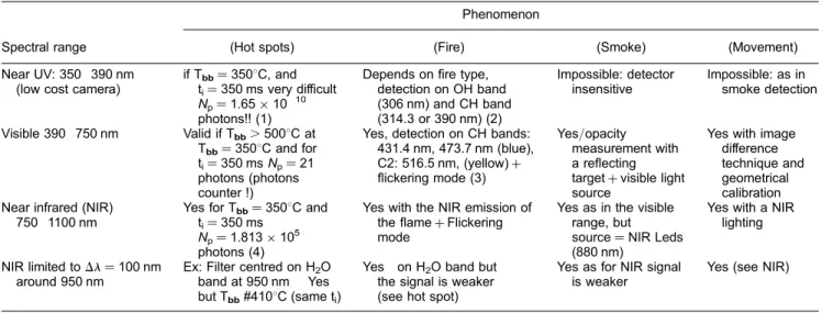
Basically, a CCD camera can be used in different spectral bands: UV (0.25–0.39 mm), visible(0.39–0.75 mm), NIR (0.75–1.1 mm) or also on a very narrow spectral filter for specific applications; therefore the next section is devoted to the comparison of these last spectral channels towards the detection of fire events: hot spots (smouldering combus-tion), flame, smoke generated by hidden fire or movement of objects or person. At first, preliminary tests were realised on a Sony silicon CCD detector with 752 # 582 pixels with a size of the CCD array equal to 6.35 # 4.83 mm and using a Wrat-ten 87 C Kodak NIR Filter, to get the lower threshold of detec-tion in energy in the NIR. For that, an optical bench and a Blackbody were used to calibrate the system as shown in Figure 3.
The graph, in Figure 3, shows that the lower limit of detec-tion (in blackbody temperature) is close to 3508C for exper-iments made in a dark room. Then, by using computations, we have investigate the advantages and drawbacks of the NIR range compared to UV or visible range of the CCD spec-tral response versus the following phenomena: hot spots, fire, smoke (another marker of a fire) and movement (of appar-atus or person). These considerations are reported in Table 2.
In Table 2, Tbb represents blackbody temperature and ti, the integration time used in the computation, (1) and (2) are just proposals for a Silicium CCD sensor using a narrow band filter. In fact, a low cost system (non-scientific grade) could be certainly not enough sensitive in this spectral range, (3) will be more feasible with an ordinary colour CCD camera. The important flame bands quoted here are
Table 1. Integrated atmospheric transmissiontatm(Dl) for different spectral ranges. Spectral range (Dl) 0.75 1 mm(NIR) 1 3 mm 3 5 mm 5 8 mm 8 12 mm Integratedtatm (Dl) . 0.95 0.75 0.78 0.19 0.93
issued from Gaydon and Wolfhard (1979). We do not include the solar blind UV band between 240 and 280 nm where this kind of detector is irrelevant. The result (4) was computed from a simplified radiometric equation at Tbb (reference) equal to 3508C, the value Np¼ 1.813 # 105photons, which is the number of photons integrated by the camera, gives us a useful threshold that we used in the other cases (e.g., with the 950 nm filter) to obtain a new Npand then, from a computed calibration curve, a new minimum detectable temperature. The 950 nm filter is proposed there because of the weak 950 nm weak water vapour emission band exist-ing in a typical hydrocarbon flame: accordexist-ing to Gaydon and Wolfhard (1979), the emission of flame in the NIR is mainly due to water vapour and soot particles (carbon emission). The trends of Table 2 confirm the choice of working in the
complete near infrared spectral band to get the maximum of energy and to optimize the different ways to detect a fire. In addition, the lowest minimum detectable temperature close to 3508C, is also quoted in the literature by Drysdale (1996): the spontaneous ignition temperature of a solid material depends on thermal boundary conditions on this typical material (flux, temperatures, radiation, convection); Table 3 gives some values for wood.
SI corresponds to a spontaneous ignition and PI depicts a piloted ignition in laboratory conditions. In Table 3, the mean temperature is equal to 4608C and the lowest 3008C, so the preliminary test of our CCD camera shows that the range of temperatures proposed is adapted to the fire detection and can operate an ‘early’ test during the hot spots phase around 3008C to prevent an operator of the probability of
Figure 3. Optical bench and response curves of the CCD camera.
Table 2. Ability for detection of phenomena respect to the different spectral bands of a CCD array.
Spectral range
Phenomenon
(Hot spots) (Fire) (Smoke) (Movement) Near UV: 350 390 nm
(low cost camera)
if Tbb¼ 3508C, and ti¼ 350 ms very difficult Np¼ 1.65 # 10 10 photons!! (1)
Depends on fire type, detection on OH band (306 nm) and CH band (314.3 or 390 nm) (2) Impossible: detector insensitive Impossible: as in smoke detection Visible 390 750 nm Valid if Tbb. 5008C at Tbb¼ 3508C and for ti¼ 350 ms Np¼ 21 photons (photons counter !)
Yes, detection on CH bands: 431.4 nm, 473.7 nm (blue), C2: 516.5 nm, (yellow) þ flickering mode (3) Yes/opacity measurement with a reflecting target þ visible light source
Yes with image difference technique and geometrical calibration Near infrared (NIR)
750 1100 nm
Yes for Tbb¼ 3508C and ti¼ 350 ms
Np¼ 1.813 # 105 photons (4)
Yes with the NIR emission of the flame þ Flickering mode
Yes as in the visible range, but source ¼ NIR Leds (880 nm)
Yes with a NIR lighting
NIR limited to Dl¼ 100 nm around 950 nm
Ex: Filter centred on H2O band at 950 nm Yes but Tbb#4108C (same ti)
Yes on H2O band but the signal is weaker (see hot spot)
Yes as for NIR signal is weaker
smouldering combustion or hazardous situation in the ware-house or any local to be monitored. At last, to describe accu-rately the physical response of our camera, a radiometric model has been developed. This model takes into account parameters such as the integration time ti of the camera which allows to cover a large energy range of phenomenon (hot spots, fires of different kinds), pixel size, numerical aper-ture of the optical system, spectral response of the camera in the near infrared, transmission of the optical system. The main results of this study, are well described in Sentenac et al. (2003) where the effect of the external temperature on the drift of the calibration curves was corrected by compu-tation and using of a thermal sensor mounted near the detec-tor to monidetec-tor the temperature inside the case of the camera, and applications of the calibration model of the camera in Sentenac et al. (2002). According to that, the most important result of this work for the application described in this paper is that the minimum detectable blackbody temperature is equal to 3308C for an integration time tiequal to 360 ms and an aperture number of 1.4 for a 16 mm focal length and that our system optimizes automatically the choice of ti for a best measurement range. As a consequence, the typical detection sequence we chose is: at first, a hot spot detection mode is activated on a blackbody temperature threshold (3308C). If this detection is positive, the system has to track if the ‘marked’ phenomenon goes to fire mode [Tblackbody. 6008C, as described in Sentenac et al. (2002)]. Then the fire detection algorithm is triggered. If the result of the detec-tion is positive, an alarm is sent to the control system and operators, if not, the smoke detection algorithm is triggered at last. This mode can also provide an alarm (hidden fire) or, if nothing is detected, return to the hot spot mode. We describe in the next section the different steps of the fire detection method.
THE FIRE DETECTION METHOD
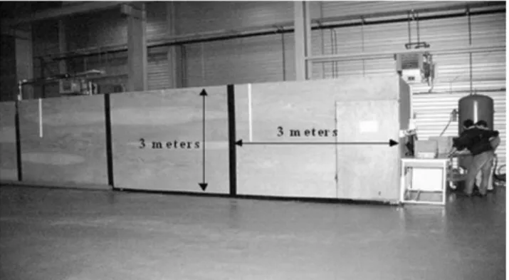
We describe, now, the different experimental benches and methods achieved in our laboratory to develop and test the fire detection algorithm. The benches were installed in a specific dark enclosure of 3#3 # 13 m to avoid perturbations coming from the environment (light, smoke, persons). This enclosure is shown in Figure 4.
To define ‘normalized’ fire and non-fire sources for the tests, we used two specific standards: the French AFNOR EN54 (1997). This standard describes particular tests on solid combustibles fires, the second standard is issued from the aeronautic domain: the JTSO–C79 (1991). This second standard was chosen here because it gave accurate descrip-tions of tests on typical non-fire sources.
Then, the experimental setup was designed to produce the following events:
1) Solid materials fires: such as paper, cardboard, wood, (typically, from EN 54 standard, 10 beech samples of
10 mm # 10 mm # 200 mm per fire or 120 g of wood). This kind of fire was produced in an apparatus composed of a con-tainer and a metallic grid on which the samples were dis-posed. This system was able to produce smouldering or fully developed combustion.
2) Hydrocarbon fires (liquids): these fires are produced in a 120 mm diameter ceramic pan, the liquid quantity was adjusted to 100 ml. The main liquids tested are hydrocarbon such as A gasoline, which produced a smoky and yellow luminous flame, or solvents like acetone or ethyl alcohol which produced a pale and bluish flame.
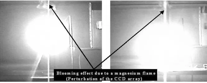
3) Non-fire sources or artefacts: these sources can simu-late phenomena which look like a fire by, at least one particu-lar parameter, as examples: radiative energy for fixed lamps, periodic emission such as flashing/periodic lamps or daz-zling light such high energy lamps or magnesium ribbon. We have to mention that these combustibles or light events are numerous on industrial sites or warehouses and that our benches lead, in this way, to realistic tests. The mag-nesium ribbon was mainly used to provide blooming or smearing on the CCD sensor as the sun or arc lamps can do (Figure 5).
This experimental setup can be seen in Figure 6(a) and (b). Figure 6(a) shows the global system and Figure 6(b) shows a closer view of the apparatus used to produce peri-odic non-fire sources: a rack composed of different lamps (red and yellow and a high power 1000 W lamp, from the JTSO-C79 standard) associated with a rotating disk including slits called a chopper. This device can produce a flashing light with frequencies in the range [1–50 Hz]; this periodic light can mimic a pulsating flame and then mislead the detec-tion system. To go further, we have to recall some important features related to the fire phenomenon. In next section, we deal with the typical flame structure associated to a prelimi-nary classification of potential detection parameters (energy and temporal aspects). Then we treat of the relevance of each of these parameter. Figure 7 presents aspects of the different zones of a classical diffusion or ‘natural’ flame recorded during our experiments. This leads to a set of poss-ible parameters to distinguish a fire from a non-fire source with a CCD camera:
Two particular regions of this diffusion flame are visible in Figure 7.
1) The persistent flame which corresponds to the bottom of the fire: the flame is always present in this particular zone.
Table 3. Flaming temperatures for wood. Heat transfer mode Surface temperature (SI) Surface temperature (PI) Radiation 6008C 300 4108C Convection 4908C 4508C
2) The intermittent region which corresponds to a zone where the flame is not always present. The upper non-visible zone is called the buoyant plume: it contains the hot combustion gases such as water vapour and carbon dioxide.
As a consequence, Table 4 lists geometrical parameters issued from observations of the video sequences, most of
them are easy to compute with image analysis (Gonzalez and Wintz (1987):
1) The variation of height of the flame versus time: this feature is related to the convection and radiation effects lay down to the liquid surface, in the pan, which corresponds to the entrainment of a stream of cold air in the reaction zone and the fluctuations of the hot gases for the intermittent region.
2) The movement of the gravity centre of the flame: as shown in Figure 8, the internal circle corresponds to the apparent movement of the gravity centre of a constant source viewed by the camera. This weak fluctuation of pos-ition is mainly due to the spatial noise of the CCD array and, therefore, can be used as a threshold to distinguish a constant source from a fluctuating source in the scene.
3) The mean NIR energy on the ‘surface’: it can be com-puted (with a binarization process) on the extracted area of the flame for each image of a typical sequence. The mean
Figure 6. (a) Fire tests system, general view. (b) Experimental bench:
flame and non source fire: chopper þ lamp. Figure 7. A typical Flame structure. Figure 5. A typical blooming phenomenon due to high energy spot.
binary level, related to the mean energy integrated by the camera, is measured. This mean level depends on the inten-sity emitted by the flame which is a function of the emissivity or the thickness of the hot gases.
4) The instantaneous fluctuation of energy on the surface of a source E f (S): (in binary level): unlike point 2, this fea-ture needs only one image: the fluctuation is only tested on the surface of the flame. In the same way, the fluctuations are related to emissivity or local temperature variations of the flame.
5) The fluctuation of the surface S f (t): it is only a geo-metrical criterion. This criterion could be interesting if a very high resolution CCD array is used or for short distance obser-vations, to analyse accurately the different scales of fluctu-ation of the flame surface. In the following section, these different criteria are discussed to establish a robust detection.
Temperature Levels and Energy Aspects of the Different Phenomena
As a flame can be described with an energy radiated in the infrared spectrum, we proposed here some estimations of flame temperature regarding the dynamic range of our camera. Then, we assumed that the heat flux in watt pro-duced by the combustion of a given quantity of solid or liquid can be computed with the following expression:
PWatt Qcombustion=kJ:kg:mkg
Dtcombustion
PRadiativeþ Pconvectiveþ Pconductive (1)
where Qcombustionis the heat released by the combustion of a material or liquid in MJ kg 1, m the mass of the sample in kg and Dt the duration of the combustion in second. This power
can be estimated in many cases because Qcombustion, m and Dt are generally known. The source term P is balanced by radiation, convection and conduction in the burner. In our case, the burner were insulated and the conduction losses were neglected. The term Pradiativeis equal to 1F. FF sSF.s. (TF4 Ts4), where 1Fis the emissivity of the hot gases, SFa mean surface of flame, s the Stefan constant, TFthe temp-erature in Kelvin of the hot gases, FF s and Ts the view factor of the flame to the surrounding, taken equal to one, and the temperature of the surrounding respectively (300 K). To compute TF, we need the value of the emissivity which is generally unknown or difficult to obtain. As an example, we made an experiment with Alcohol that appears as the less energetic fuel and then the most critical case of detection for the CCD camera, compared to acetone or A gasoline. This fuel has a Qcombustion! 27 MJ kg 1, the quan-tity of liquid burnt was 20 ml (0.016 kg), and the duration of combustion observed was equal to 130 s; this led to a power released equal to 3320 watts. Neglecting the convec-tive effect in a first approach, assuming that the flame acts as a blackbody (1F¼ 1) and that the surface of flame is closed to a an approximate cylinder of 0.2 m height and 0.1 m in diameter, estimated from video tapes analysis, we get a rough estimation for TF! 980 K; Drysdale (1996) gives a value closer to !1500 K.
As a result, this first estimation of the flame temperature indicates that the most critical fuel would be detected by a NIR CCD system (as we saw earlier, the threshold blackbody temperature is !600 K). But, due to the lack of data on flames such as effective surface or measured equivalent blackbody temperatures, we have established an experimen-tal database including geometrical and thermal parameters such as equivalent mean blackbody temperatures measured in the NIR with the CCD camera for each phenomenon (flames, lamps). This database uses the calibration curves of the camera in the NIR infrared made on a 500–15008C Land Blackbody and for an integration time ti of 0.1 ms. These blackbody temperatures are listed in Table 5.
The apparent blackbody temperature for the magnesium ribbon was found equal to 1162 K. Hence, except for the
Figure 8. Gravity centre criterion.
Table 4. Fire detection criteria.
Phenomenon/criterion Fire Non Fire:Lamp þ chopper Non Fire: lamp (1) Height ¼ F(t) Variable Constant/periodic Constant (2) Movement of the gravity centre Variable versus time Weak variation during the flashing phase Fixed (3) Mean NIR energy E on the surface S Variable versus time Two different values: dark/bright Constant
(4) E ¼ F(S) Variable Constant Constant
(5) S ¼ f(t) Variable Variable Constant
Table 5. Equivalent blackbody temperatures of phenomena measured with the CCD camera.
Phenomenon Candle flame A Gasoline Ethyl Alcohol Acetone Temperature (K) 1154 1159 1022 1153
Phenomenon Methanol Wood Red light Yellow light 1 kW lamp Temperature
(K)
771 1108 1101 1141 Out of range
methanol flame which is nearly invisible, all the apparent temperatures found were greater than 6008C, the higher limit implemented in our hot spot detection algorithm.
Analysis of the Geometrical Characteristics of Fires: Dimensional Aspects
In this section, we have analysed the size of fires com-pared to the field of view of the sensor used in our exper-iments and we deduced the best criteria for the detection. We have also compared the experimental results to compu-tations in order to prevent overheat aspects and security pro-blems related to the bench specifications.
It is possible, knowing the heat of combustion of solids or liquids, to compute the height of flames from dimensional analysis applied to experiments on thermal plumes emitted by a fire. This approach, at first, was proposed by Zukoski et al. (1984), who shows that the mean height of the flame depends on the diameter of the burner and the dimensionless heat of combustion with:
Qd
Qf
r1Cp1T1pgD:D2 (2)
where Qfis the power released by the combustion of a given quantity of product, r1, Cp1, T1, respectively the specific volume (far of the heat source), the heat capacity and the temperature of air taken at 208C. Equation (2) used also the diameter of the burner (or the pan) and g is the gravita-tional acceleration. With T ¼ 208C and D ¼ 0.12 m, we get Qd¼ Qfx1.864 # 10 4. By using a graph and large number of values of Qd, it is shown in Zukoski et al. (1984) that the plot of Hmean/D¼ f(Qd) is nearly linear but two different regions can be distinguished (two slopes) according to the value of Qd, that is to say:
Qd, 1, HmoyD % 3:3:Q 2=3 d Qd& 1, HmoyD % 3:3:Q2=5d ( (3)
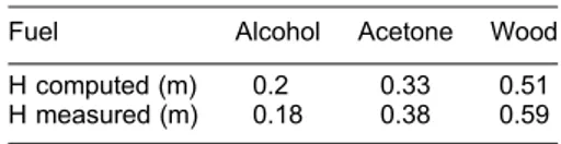
We gathered the different values obtained for different fires on our experiments. These experiments were made here with a camera lens focal length of 8 mm. This focal length was chosen to provide a large field of view in order to mini-mize the number of sensors to cover a given surface. As a result, for the critical distance of 10 m in our dark cell, the maximum available for our configuration, the horizontal field viewed by the camera was 7.9 m and the vertical field was 6 m. Then, we have compared the computations from equation (3) to experiments. The values of height, at the beginning, given in pixels from image analysis were con-verted into height in meter from geometric calibrations. This comparison is given in Table 6 for fuels where chemical data are available.
The mean relative error is closed to 13% for all flames. The order of magnitude is correct and useful to estimate the
height of a flame for a given quantity of combustible and size of burner. The measurement for the wood experiment gave a mean area contained in a rectangle of 56 # 36 pixels and for the alcohol, 11 # 19 pixels: the areas of phenomena are included in the range (209& area &2016) square pixels.
Now, if these areas are compared to the global surface in square pixels of the CCD array: 437 664 square pixels, the phenomena of interest represent in the best case, 0.46% of the area of the detector or in the worst case 0.047%. The viewed fluctuating zone is very weak and then we were here in the most critical case of detection very close to real situations.
Analysis of the Fluctuating Mode of Fires
As we said, the use of a CCD sensor in the near infrared spectral band was not consistent with a pure spectral analy-sis. Then, related to the integrated energy emitted by a fire and its variations, we studied the most relevant criterion for the detection.
1) Radiative flux variation: considering, at first, the flux vari-ation emitted by the hot gases at high temperature: if the gases are isotherm, the flux emitted in the NIR band is described by the following expression:
F F0:(1 e'K:L) with F0 f :SF:s:TF4 (4)
F0is the fraction of the global flux emitted at the real flame
temperature TF in the spectral range of (0.75–1.1 mm) ( f , 1) and SFthe surface of the flame, s is the Stefan con-stant and 1F¼ 1 e K.L is the emissivity of the hot gases with K the integrated absorption coefficient in m 1 of the hot gases in the NIR and L is the geometrical thickness of the flame.
Expression (4) can be transformed to: dF F K:L:e'KL 1 e'KL: dL L ð5Þ
With a review of the different values of K from the literature (Drysdale, 1996), we have computed the value of the function:
F(x) (x:e'x)=(1 e'x) with x ¼ K.L called the optical
thickness (Brewster, 1992) and L % 0.1 m. The results are presented in Table 7.
For x ¼ 1,we get F(x) ¼ 0.58. From the previous results, it was possible to distinguish two cases:
a) The flame is optically thick, i.e., dF=F % a:dL=L with a * 1 and the relative variation of thickness has not a great influence on the emitted flux even if the real thick-ness of the gases presents important variations, the intensity viewed by the camera seems to come from a
Table 6. Flame heights (dimensional). Fuel Alcohol Acetone Wood H computed (m) 0.2 0.33 0.51 H measured (m) 0.18 0.38 0.59
Table 7. Optical thickness influence.
Fire A gasoline (!) Acetone Alcohol Wood
x ¼ K.L 0.35 0.14 0.07 0.065 F(x) 0.835 0.93 0.965 0.967
!Optical properties are taken very close to kerosene ones (Drysdale,
layer of thickness Lp % 1/K called the photon mean free path with Lp * L.
b) The flame is optically thin, then dF=F % dL=L, K.L vanish to 0, the relative variation of the emitted flux is directly proportional to the relative variation of thickness dL/L.
We have compared this approach to measurements realized on three kinds of flame. At first, we have analysed the thick-ness by considering the diameter of the burner and assuming that the fluctuations of ‘width’ observed on NIR video sequences were, in a first approach, 2D axisymmetric. Then, the standard deviation s of these fluctuations has been compared to the fluctuations of binary levels recorded on the same images.
These parameters are listed in Table 8.
As a result, the mean value of the relative variations is equal to 16.4%. The corresponding variation observed on the binary levels from image analysis on area of interest are close to 10%. From Table 7, the mean value for x is !0.16 for all flames which gives a corresponding value for F(x) ! 0.9 (optically thin mode). Then with the mean relative variation of thickness and the last value of F(x), we found a computed dF/F ! 15%. This value is a little greater than the 10% really measured on the image in levels variations. So, in all case the variations on the energy level appeared to be weak. In the same condition and for the same flames, the height parameter appears more consistent.
From Table 9, the mean value of the height parameter for the three flames is then equal to 30%, a value twice greater than the value found in the thickness variation for a given distance.
2) Analysis of the fluctuation of the area of the flames due to the hypothetic position of a fire toward the camera: We saw that the relative variation of area remained always weaker than those of the height: 25% against 30%. Then the evol-ution of the area of the flame viewed by the camera at a given distance Ddcan be written with the following expression:
Sd(square Pixels)
Dd
Dref
" #2
:Sref(square pixels) (6)
where Sdis the area of the phenomenon at a distance Ddand Srefis the area of the same phenomenon at a distance Dref (reference). Then we saw that, for the alcohol flame, the mean number of square pixels at 5 m is 131, at 10 m this sur-face decreases to 33 square pixels. The relative variation of the area dS/S remains the same at any distance. For the alco-hol flame, we found 30.5%, then absolute fluctuation at 10 m was dS10 m¼ (30.5/100)!33 ! 10 square pixels. We can com-pare this value to the total number of square pixels on the array of the camera: 752 # 582 ¼ 437 664 square pixels. The effec-tive variation of area become 0.002% of the array. Thus the dis-crimination on the fluctuation of the area of interest can be used only at very short distance (if fluctuations are noticeable). As a
result, the height parameter appeared as one of the best par-ameter to make the discrimination for fire detection in our case. 3) Analysis of the height parameter: About this aspect, the literature deals mainly with a specific frequency of pulsation of the height of flame for pool fires related to convective instabil-ities. Some authors (Uber das Flackern von Flammen, 1971; Chitty and Cox, 1979) give empirical relation between the diam-eter of the burner (or pool fire) and the typical frequency of pul-sation of the flame. In order to study this frequency of pulpul-sation, we made experiments with several combustibles. We show in Figure 9 the height spectra of flames plot with a fast Fourier transform (FFT) computation on the height parameter. The three flames were acetone, alcohol with a 12 cm pan and a wood fire with the same burner size.
We gathered our data issued from Figure 9 and the ones from the literature to provide a comparison in Table 10.
We noticed that the mean relative difference between the data from the literature and our measurements remained weak, in general ,20%. This preliminary results led to the fact that it was possible to consider the fire phenomenon, in a first approach, as a phenomenon presenting a good rating of periodicity. This aspect is also noticeable on one of our video sequences for an acetone flame (Figure 10).
However, this situation remains an ideal situation because the flame is produced on a finite pan (12 cm diameter), this flame is nearly in steady state and far away from environment perturbation. The frequencies presented in Table 10 depend on the conditions of combustion: starting of the fire, growing and extinction. Secondary groups of frequency are present on spectra of fires, they are related to slow pulsations of the basis of the fire. This first results led us to test a first
Table 8. Measured flame thickness and fluctuations. Fire A gasoline Acetone Acohol Measured thickness ¼ width (pixels) 31 29 17
sthickness (pixels) 4.6 3.7 3.7 (sthickness/thickness)!100 in % 14.8 12.7 21.7
Table 9. Measured flame heights in pixels.
Fire A gasoline Acetone Alcohol height in pixels (H) 58 51 24
sheight pixels 16.4 11.8 9.4 (sheight
˙/H)
!100 in % 28 23 39
periodicity criterion for the fire detection process. This cri-terion used the FFT computed on the height parameter of the flame. This criterion is defined with the following items: . Acquisition of a sequence of N images, N can be equal to
64 images (video rate 25 Hz) for laboratory tests, and 32 images (25 Hz) for compact industrial system with less dynamic memory.
. Automatic threshold step to obtain a sequence of binary images, the height of the flame Hifor each image i of the sequence were extracted.
. Computation of a FFT, then on the energy spectrum of Hi, the maximum of energy E were searched to find the fre-quency of the first harmonic F1 and the others k.F1until to the highest frequency of the spectrum, 12.5 Hz in our case (with a frequency increment equal to 0.39 Hz or 0.195 Hz). The residual energy E at the other frequencies given by k.F1þ(F1/2) which is non-zero if the phenomenon is non periodic.
. Computation of the periodicity criterion using equation (7) from Polana and Nelson (1997):
P PNharmonics k 1 E(kF1) PNharmonics k 1 E(kF1þ F1=2); ; PNharmonics k 1 E(kF1) þPNharmonicsk 1 E(kF1þ F1=2) , 0 & p & 1 (7)
Equation (7) was tested, at first, on known signals (numeri-cally built). These signals were generated on 64 points in order to reproduce the same sampling conditions as for the flames. The test signals were respectively square sig-nals, sinusoids or sinusoids with noise (amplitude of noise was equal to the half of the sinusoid). For a sampling rate of 40 ms (25 Hz), the frequency simulation is then 0.39 Hz and for the full spectrum, the range of frequency is (0–12.5 Hz). The frequency of the numerical signals was in the range (1–10 Hz). The value of the periodicity criterion obtained for noiseless signals was always greater than 0.9. For the noisy signals this value was close to 0.4. These results are presented in Figure 11.
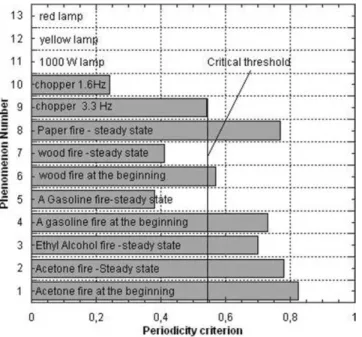
Then, this criterion was tested on real signals extracted from fire sequences (64 frames) and chopper sequences with frequency in the range (0–5 Hz) which corresponds
to realistic ‘puffing’ frequencies for burner size of 0.12 m. These results are shown in Figure 12.
Figure 12 shows that it was difficult to distinguish a real fire among non-fire sources.
It shows that, the critical threshold chosen here as the highest value of P for non-fire sources is greater than two fire sources (wood, and A gasoline at steady state). Moreover, noticeable variations of P can be observe depending if the fire source is at the beginning, at the steady state or close to the extinction. Then, due to this dif-ficulty, it was necessary to implement a more selective cri-terion which was an intermittency cricri-terion of flame height (Zukoski et al. 1984). This method is based on the analysis of the flame presence probability at a specific height. For a sequence of N images, the first step is to compute the flame height Hf for each image of a sequence and the mean value of the flame height Hmean. In a second step, the ratio Xi¼ Hf(i)/Hmeanfor each image of the sequence (i ¼ 1,. . .,N) is provided. The third step consists in the
Figure 10. A typical ‘puffing flame’.
Figure 11. Periodicity evolution for synthetic phenomena. Table 10. Puffing frequencies of flames (from finite geometry).
Fire/burner size:
diameter 12 cm F(Hz) main group F(Hz) secondary group
F ¼ 1:5= Dp , D in m (from Chitty and Cox,
1979)
F ¼ 1:42=D0:65, D in m
(from Uber das Flackern von Flammen, 1971) (fit on data)
Acetone 4 !1 and 7 10 Hz 4.3 5.6
Alcohol 4.8 !1 4.3 5.6
comparison of each Xi to Xjfor each image of the same sequence ( j ¼ 1,. . .,N). As a result, if Xj. Xj, a variable NIis incremented. At the end of the j loop, the normalized intermittency If(i) ¼ NI/N is computed.
If Xiis very low, then Xjis always greater than Xi, NIgoes to N; as a result If(i) goes to one. This specific effect means that the flame is always in the persistent region. On the other hand, if Xi is high then Xj stays in the major cases under Xi, NI goes to zero; for this case, the flame is in the buoyant region: the probability that the flame reaches this region is weak.
At last, step 3 of the algorithm is an ascending sort of the Xi and a descending sort of the If(i). The value at Xi¼ 1 represents the typical signature of intermittency (I) for a given fire. This can be seen in Figure 13.
By applying this algorithm to different fire sequences and plotting the results on a global graph (Figure 14), we show that intermittency is a reproducible characteristic of fires.
This implies that the different values of intermittency for fires can be very close and appear as a consistent par-ameter for detection as shown in Figure 15.
This figure presents a comparison between fire and non-fire sources for the intermittency I. The mean value of I is equal to 0.472 for fires and the associate standard deviation s equal to 0.047. The main part of the values of fires lies inside the range (Imeanþ 1.5s, Imean 1.5s) compared to the value non-fire source which lies in the range (0, 0.22) except magnesium ribbon flame, which is related to bloom-ing effect of the CCD array. This point improves the ability of detection. As we can see this parameter was chosen for its simplicity and reliability.
But to make the detection more robust, it was necessary to consider a multi-criterion detection as we explained in previous sections. Then a second criterion was extracted from Figure 7 and Table 4.
This new criterion is based on a measurement of the movement of the source, more precisely on the movement on the centre of gravity of the source. For that:
. In a first step, a typical sequence of 32 images was ana-lysed and for each image, the centre of gravity (Xi, Yi) of the area of the source was computed and the results were recorded in a file [Xi, Yi].
. The second step was to compute the centre of gravity of the entire file [Xi, Yi] that is to say (Xg, Yg) as shown in Figure 8.
. On the third step, for each (Xi, Yi), a Euclidean distance was computed between (Xi, Yi) and (Xg, Yg) with:
Li (Xi XG)2þ (Yi YG)2
q
(8)
Figure 14. Comparison of intermittency graph for several fires. Figure 12. Comparison of periodicity criterion for real phenomena. Figure 13. Intermittency graph for a typical fire (acetone).
A computation using equation (8) was made, at first, on a set of non-fire sources which gives a subset of fLig, then a parameter RB¼ maxfLig was computed. As a result for a fixed source, for example a lamp, RBcorresponds to a maxi-mal radius of fluctuations; which is, in this particular case, only dependant on the spatial noise of the CCD sensor.
. At last, the same computations (8) are done on fire sequences and chopped light and if Li . RB for the image I, then a parameter Bxy is incremented and at the end of the computation, the rate of ‘movement’ of the centre of gravity of the phenomenon is given by Nmovement¼ Bxy/Nimages.
As a result, like the intermittency parameter, this new criterion Nmovement is in the range [0,1]. This aspect can be seen in Figure 16.
This graph presents three different features:
. The fluctuations of a steady lamp source are limited to the spatial noise of the CCD sensor (the radius of the amplitude of fluctuations are low).
. The chopped light is characterized by two regions on the graph corresponding to the sequence of periodic light. In practice, the movement criterion is not com-puted during the dark part of the sequence to avoid spurious values of Xgand Yg.
. A flame shows a distribution of points nearly rectangular with DYg. DXg(DXgwere weak on our flames). However, in our optical system the depth of field is fixed and set on the range [2 m-1] (2–10 m in our experiments). The move-ment criterion was computed, in the precedent section, for a middle range distance of 5 m. Nevertheless the real localization of a fire event is generally unknown: the fire can start every-where between 2 and 10 m. It was necessary to modify the threshold of the movement criterion for the worst case: with a value of RB, for a typical distance of 5 m, equal to 0.122 pixels when fixed lamps are observed, we have to compute this new RB in out of focus situation. At 2 m, with simple projection relation using DD ¼ (Dv/f). dd, where f is the focal length of the optical system (lens) Dvis the distance of observation of the phenomenon and DD, dd are the geometrical size in the object plane and image plane respectively; we got RB¼ 0.3 pixels. Finally, the movement criterion was tested with this new value of RBand was found equal to nearly one for fires sources, 0.87 for choppers and 0 for fixed lamps. This first cri-terion indicated that the discrimination between choppers and fires was poor: DBxy/Bxy! 13%. We deduced that chopper did not mimic an ideal square wave and it was necessary to introduce an additional test in the computation of Bxy: we saw on a typical sequence of chopped light, that the binary level varied between a saturated value, due to the high flux of the 1000 W lamp used in the tests, when the lamp was visible and a dark level when the light incoming from the lamp was inter-rupted by the blade of the chopper. So, a reference image of the ‘dark’ scene was recorded to get the higher dark level in this reference image. This led to conditional computation of the cri-terion: if the current binary level of a sequence became is minor than the higher reference dark level, the criterion was not computed (that means that the source is not visible). With this new condition, we found that the movement criterion was equal to 0.258 for chopper sources. it was then possible to dis-tinguish the different phenomena (Table 11).
In Table 11, Tebrepresents an equivalent blackbody temp-erature issued from the a calibration curve used by the hot spots detection algorithm (radiometric model). This tempera-ture must be always greater than 6508C, for the complete sequence recorded for the test. For (1) and (2) the practical thresholds were .0.5 and ,0.5, respectively. In addition, the algorithm creates one region of interest (ROI) per phenomenon detected in the scene. For each ROI, a set of
Figure 15. Results of the intermittency analysis (all phenomena).
Figure 16. Ygversus Xg.
Table 11. Final values of detection thresholds.
Criterion/phenomenon Fire sources Chopped lights Lamps Teb .6508C .6508C .6508C I [ ½0:4,0:56, [ ½0,0:22, 0 Bxy .0.9(1) & 0:258(2) 0
three parameters is computed: Teb, I and Bxywhich allows us to classify the different phenomena. Hence, it was possible to plot a graph of intermittency I versus Bxy(Figure 17).
The drawing of this set of values allowed us to define a straight line to classify the region of fire sources and region of non-fire sources. This line was obtained by cumulative computation of all the tests done during our experiments. The criterion used to draw this line is obtained by the follow-ing expression:
Test ¼ a.Bxy-Intermittency þ b where a and b are deter-mined by a graphical method to give a ¼ 1 and b ¼ 1.1 (the straight line on Figure 17 is only a schematic one). Then, for a couple of values, if the parameter Test .0, the phenomenon is a non-fire source, for Test ,0 the phenom-enon is associate to a fire source. When the resulting value of Test is zero, the phenomenon is recorded and classed as a limit case (undetected). The decision can be facilitate for an operator, by presenting the results of the algorithm and the associate video sequence (the ultimate information for decision). In future work, it could be possible to improve the detection by moving slightly the frontier of the threshold by a machine learning technique. In addition, to test the system in severe conditions, we chose to configure the algor-ithm in mono-ROI mode and to perturb the detection by acti-vating several phenomenon at the same time in the scene. For example, a fire and a lamp very close in position. We show in Figure 18 the preliminary results of these tests.
This plot shows two regions which can be separated with a threshold between a fire and a non fire region. Some numeric labels are related to specific situations:
(1) Regions associated with coloured lamps and high power spot of 1 kW.
(2) Point associated to the combustion of a magnesium ribbon: the movement criterion equal to 0.65 due to movement of ribbon during the flaming phase but no intermittency was recorded (the flame appeared as a brilliant and constant white spot).
(3) The choppers region.
(4) An acetone flame close to a 1 kW lamp. (5) Acetone flame beside red and yellow lamps.
(6) Fire region (pure, non-perturbed), the lower part of this region (I ¼ 0.4, Bxy# 0.95) corresponds to a wood fire perturbed by the opening of the door of the dark enclo-sure (shown in Figure 4) near the burner.
Then these perturbations modify slightly the detection par-ameters while keeping the ability of detection. As an example, the case of a fire beside a lamp which is switched on: the algorithm, forced to monitor only one ROI, binarize a region which contains a fire and a lamp. This leads to decreasing (38%) the intermittency parameter. These smoothing effects tend to disappear when a ROI is affected to every phenomenon detected in the scene. Then the detec-tion remains fair for most of the fires with a weak effect of the observation distance: for an alcohol flame, a variation of 11% is observed on the intermittency parameter I by vary-ing the distance between the fire and the camera in the range (2–10 m); in the same condition, the variation observed on the Bxyparameter is only 3.1%.
CONCLUSION AND FUTURE WORK
In this paper we have presented a new method of fire detection involving a near infrared CCD camera. After a short part dedicated to the performances of the camera in the near infrared (radiometric model), we have presented some aspects of the state of the art for fire detection systems: from classical thermal sensors to up to date video tech-niques. In every cases, we have shown that the detections implemented were not complete. Then we have justified, with an energy comparison, the choice of the near infrared spectral band among the full spectral response of the CCD camera to satisfy to fire precursor detection (hot spots) and flame detection. This choice is the result of a compromise between geometrical aspects and signal-to-noise ratio. The experimental setup used in our experiments is described: a large dark enclosure with multi-purpose optical test benches. Afterwards, with considerations on the morphology of flames issued from video sequences on real fires, the choice of the best criteria of detection was studied: height fluctuations,
Figure 17. Intermittency versus Bxy.
effect of the thickness of the hot gases, movement of the flames, energy fluctuations.
From this part, three parameters were fixed: height fluctu-ations, movement of the flame around its gravity centre and energy level. A first approach based on a periodicity criterion for the height was tested, from an outstanding feature observed on some of our video sequences and confirmed by literature data such as the ‘puffing’ mode of combustion (peri-odic flickering of flame for a given geometry of burner). But this approach was not relevant (weak reliability) and far from a real situation of fire. Then a more realistic analysis using the intermittency criterion was proposed and performed on tests for the different criteria chosen, mainly to implement the best threshold value in each case to separate real fires from non-fire phenomena such as lamps, ray of lights incoming from holes, windows. The preliminary results of the algorithm proposed are presented: even in perturbed situation (several phenomena in the scene, opening of a door in the dark enclo-sure), the detection remained effective and robust. Finally, a three parameters algorithm: intermittency, movement of the gravity centre of the flame and its equivalent blackbody temp-erature taken as a critical level was used to produce fair results with a detection time ,3 s, for flames size down to 0.15 m # 0.1 m at 10 m of the CCD camera. This algorithm was also completed by a smoke detection algorithm (precursor or non directly visible fire) well described in Sentenac et al. (2004). For the future, in the field of fire detection, new extents of the method proposed in this paper are considered to treat more industrial sites than a simple dark warehouse, such as tunnels, plants, where additional lights or other non-fire sources are always presents. Then new tests and adapted learning phase will be necessary to enlarge the possibility of the algorithm. We are also working on the improvement of the radiometric model for a new camera in the near infrared as explained in Rotrou et al. (2006). For that, a specific soft-ware was developed to use this kind of camera to perform near infrared thermography in the domain of material science by taking into account the relevant parameters in the measure-ment such as emissivity, reflectivity, transmissivity of windows or particular media in front of the CCD sensor. Applications devoted to analysis of reactive flows in laboratory situation are also considered.
REFERENCES
Association Franc¸aise de normalisation (AFNOR), 1997, European Requirements for Industrial Fire Warning Systems (in French): “Organes constitutifs des syste`mes de detection automatique d’incendie, partie 9, essais de sensibilite´ sur foyers types”. Bedat, B., Giovannini, A. and Pauzin, S., 1990, ‘Instantaneous temp
erature profile measurements in a flame by infrared line thermome try technique’, Eurotherm Seminar N817.
Brewster, Q., 1992, Thermal Radiative Transfer and Properties, (J. Wiley).
Chitty, R. and Cox, E., 1979, A method of measuring combustion intermittency in fires, Fire and Materials, 3: 238 242.
Drysdale, D. 1996, ‘An Introduction to Fire Dynamics’, (Wiley Interscience, John Wiley & Sons).
Gaydon, A.G. and Wolfhard, H.G., 1979, ‘Flames, Their Structure, Radiation and Temperature’, (Chapman and Hall, London, UK). Goedeke, A.D., 1995, ‘Cost effective, dual purpose machine vision
based detectors for (1) smoke and flame detection, and engine overheat/burn through and flame detection’, Final Report (WL/ FIVS, Technology Section, Survivability and Safety Branch, Vehicle Subsystems Division, Wright Patterson Flight Dynamics Laboratory, WPAFB OH, USA).
Gonzalez, R.C. and Wintz, P. (ed.), 1987, Digital image processing, (Addison Wesley).
Hayakasa, H., 1996, ‘Radiative characteristic and flame structure of small pool flames’, FireTechnology, 32(4), 308 322.
Joint Technical Standard Order (JTSO C79) 1991, Joint Aviation Requirements, (FAA, Washington DC, USA).
Lloyd, A.C., Zhu, Y.J., Tseng, L.K., Gore, J.P. and Sivanthanu, Y.R., 1998, Fire detection using reflected near infrared radiation and source temperature discrimination, NIST report, NIST GCR 98 747. Pfister, G., 1997, ‘Multisensor/multicriteria fire detector: a new trend rapidly becomes state of the art’, Fire Technology, 33(2), 115 139. Phillips, III, W., Shah, M. and da Vitoria Lobo, N., 2000, ‘Flame recognition in video’, Fifth IEEE Workshop on Applications of Computer Vision, 224.
Plumbs, O.A. and Richards, F., 1996, Development of an economical video based fire detection and location system, NIST report, NIST GCR 96 695.
Polana, R. and Nelson, R., 1997, Detection and recognition of periodic, non rigid motion, International Journal of Computer Vision, 23(3), 261 282.
Sentenac, T., Le Maoult, Y., Orteu, J.J. and Boucourt, G., 2002, A video based sensor for Aircraft cargo area surveillance, Optical Engineering, 41(4), 796 809.
Sentenac, T., Le Maoult, Y., Rolland, G. and Devy, M., 2003, Temp erature correction of radiometric and geometric models for an uncooled CCD camera in the near infrared, IEEE Transactions on Instrumentation and Measurements, 52(1), 46 60.
Sentenac, T., Le Maoult, Y., Orteu, J.J. and Boucourt, G., 2004, Overheating, flame, smoke and freight movement detection algor ithms based on CCD camera for aircraft cargo hold surveillance, Optical Engineering, 43(12), 2935 2953.
Rotrou, Y., Sentenac, T., Le Maoult, Y., Magnan, P. and Farre´, J., 2006, Near infrared thermography with silicon FPA comparison to MWIR and LWIR thermography, QIRT Journal, 3(1), 93 115. Zukoski, E.E., Cetegen, B.M. and Kubota, T., 1984, Visible structure
of buoyant diffusion flames, Twentieth International Symposium on Combustion, Combustion institute, 361 366.
Uber das Flackern von Flammen, 1971, 6th International Seminar on the Problems of Automatic Fire Detection, Aachen.
ACKNOWLEDGEMENT