Science Arts & Métiers (SAM)
is an open access repository that collects the work of Arts et Métiers Institute of
Technology researchers and makes it freely available over the web where possible.
This is an author-deposited version published in: https://sam.ensam.eu Handle ID: .http://hdl.handle.net/10985/9811
To cite this version :
Raphaël MOULART, René ROTINAT - Evaluation of the Penalized Least Squares Method for Strain Computation - In: SEM 2015, Etats-Unis, 2015 - SEM 2015 - 2015
Any correspondence concerning this service should be sent to the repository Administrator : [email protected]
Evaluation of the Penalized Least Squares Method for Strain Computation
Raphaël Moulart, René Rotinat
Mechanics Surfaces and Materials Processing – Arts et Métiers ParisTech – Rue Saint
Dominique BP 508 – 51006 CHALONS-EN-CHAMPAGNE – France
E-mail: [email protected]
ABSTRACT
This work proposes an alternative procedure to smooth and differentiate experimental full-field displacement measurements to get strain fields. This one, the penalized least squares method, relies on the balance between the fidelity to original raw data and the smoothness of the reconstructed ones. To characterize its performance, a comparative study between this algorithm and two other commonly implemented strategies (the 'diffuse approximation' and the Savitzky-Golay filter) is achieved. The results obtained by the penalized least squares method are comparable in terms of quality of the reconstruction to those produced by the two other algorithms, while the proposed technique is the fastest as its computation time is totally independent from the asked amount of smoothing. Moreover, unlike both other considered methods, it is possible with this technique to perform the derivation to obtain strain maps before smoothing them (while the smoothing is normally applied to displacement maps before the differentiation) which can lead in some cases to a more effective reconstruction of the strain fields.
Keywords: Full-field kinematic maps; smoothing algorithms; numerical differentiation; penalized least squares;
performance characterization
1. INTRODUCTION
Most of the full-field kinematic measurement methods (such as digital image correlation, electronic speckle pattern interferometry, grid method,…) provide displacement maps when, in solid mechanics, the useful information is normally given by strain fields (for identification of mechanical properties for instance). Consequently, the raw displacement data usually have to be numerically differentiated. However, a numerical differentiation strongly amplifies the level of noise that affects a signal. An intermediary step of smoothing is thus often necessary before proceeding to the numerical derivation.
Surprisingly, only a few smoothing techniques are currently used by the experimental mechanics community [1]: – Local data filtering by a kernel [2]. This technique provides a fast approach but does not efficiently
reconstruct the data near the boundaries of their domain.
– Global regression techniques (on a 2D polynomial function basis for instance) [3]. This approach can be efficient for very low spatial frequency signals but can induce reconstruction artefacts on the borders and parasitic oscillations within the reconstructed field when the number of parameters of the function increases.
– Global regression based on a “finite elements-like” approach [4].
– Local polynomial regression utilizing a moving weighted least squares algorithm: the so-called “diffuse approximation” [4]. This technique provides very satisfactory results (especially efficient for reconstructing the data at the boundary) but can be very time-consuming when the span of the moving least squares algorithm increases.
In order to improve the currently applied methodologies, a fast bibliographical review in statistics and data analysis literature shows that several competitive alternatives do exist. This article is aimed at adapting one of the available techniques to the processing of full-field kinematic measurements and to evaluate its performances compared to two others methods: the “diffuse approximation” (called DA later in the paper) and the
Savitzky-Golay filtering approach (called SG later in the paper). SG, if not generally used in processing full-field kinematic maps, is a very popular smoothing technique since it combines the quickness of the kernel smoothing with a local polynomial basis approach such as in DA. Moreover, it can compute directly the derivatives of a noised data set [5].
After having recalled the principle of the chosen algorithm, the penalized least squares (called PLS later in the paper), the technique is applied to several cases (an analytical 2D function, FE simulated displacement maps and actual experimental maps) and its performances compared to those of the two other algorithms. A final section concludes the paper and gives some prospects of the chosen method that could easily be extended to fit new requirements induced by the current evolution of full-field kinematic measurements (especially, the 3D tomographic measurements that are becoming more and more popular).
2. THE PENALIZED LEAST-SQUARES ALGORITHM (PLS)
The penalized least squares method is not new. It dates back to approximately a century [6,7]. A modern formulation of PLS can be found in [8,9].
The basic idea of the method is to minimize a quantity expressing the balance between the deviation of the reconstructed data from the raw noised data and the roughness of the reconstructed data. To illustrate this, let us consider a 1D data set of n observations yi made on equally spaced abscissae. One has to find the reconstructed values zi that minimize the quantity Q expressed in equation (1):
In equation (1), the term ∆d zi is the d
th
order difference of the zi values. So, the deviation term is the square of the norm of residuals and the deviation term, the square of the norm of the d th order difference of the reconstructed values. The term λ is the smoothing parameter that gives a relative weight to the roughness term in the functional
Q to be minimized: the higher value of λ, the smoother the reconstructed data.
The minimization of Q has a close-form solution. Adopting a matrix formalism, the vector of the reconstructed values {z} can be written as:
where { . } denotes a column vector, [ . ] a matrix; [ I ] is the nxn identity matrix and [Dd] the matrix such as [Dd].{z} is the d th order difference of the zi values.
As the method leads to a close-form solution, it is very fast compared to other currently used techniques.
To fit to the requirements of the processing of kinematic maps, the algorithm as to be able to deal with missing values (that can occur when regions of interest that are not rectangle-shaped are observed or when the samples present holes). This missing values result in NaNs in Matlab® or equivalent numerical analysis software. To deal with these NaNs, a weighted version of the algorithm can be set up. Each residual term is assigned by a weight wi equal to 1 for valid points and to 0 for rejected points. This leads to the reconstructed data expressed in equation (3):
(1)
(2)
where [W] is a diagonal matrix containing the wi values.
To deal with 2D data sets, [Dd] matrix has to be slightly adapted. A 2nd order differentiation operator is considered with two additional lines at the beginning and the end corresponding to a reflective boundary condition. [D2] is now
a square matrix and can be eigen decomposed leading to:
The left multiplication by [U]T and by [U] corresponds to the application of a discrete cosine transform (DCT) and inverse discrete cosine transform (IDCT) [9,10]. Equation (4) thus becomes:
Due to the properties of the discrete cosine transform, the same kind of approach can be applied to 2D equally spaced data. For a 2D grid of values, equation (5) becomes:
with DCT2 and IDCT2 respectively denoting the 2D discrete cosine transform and inverse discrete cosine transform, ○, the Hadamard product (elementwise product) and [ ΓII ] a square matrix depending on λ and the eigenvalues of the 2D version of [D2].
3. SMOOTHING OF KINEMATIC MAPS: EVALUATION OF PERFORMANCES
3.1. Smoothing of a noised map of a 2D analytical function
The performances of the chosen algorithm have been first evaluated on a noised analytical function. The advantage of using an analytical function is that one has access to the analytical derivatives which allows a comparison of the reconstructed derivatives to the actual ones getting rid of every source of error on these last values.
The analytical function that has been chosen is the “peaks” function of Matlab®. Here, a (1000 x 1000) matrix has been generated. A Gaussian noise with mean zero and standard deviation one has been added to the map which leads to a typical high resolution noised displacement maps both in terms of spatial localizations and of signal to noise ratio. Views of the raw and noised functions and its analytical derivative with respect to x are shown in Fig.1.
(a) The function (b) The noised function (c) Its derivative with respect to x
Fig. 1 : The 1000 x 1000 pixels analytical “peaks” map
(4)
(5)
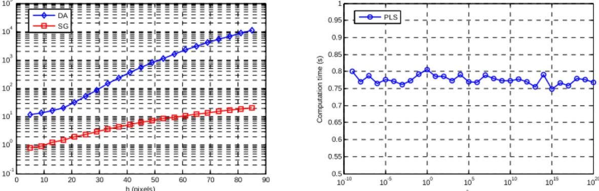
First of all, the time spent to perform the reconstruction has been looked at. The computation has been performed using Matlab® on a 64 bits computer equipped with an Intel® CoreTM i7-2760QM (2.4 GHz) CPU and a 8 GB DDR3 1333 MHz RAM. The computation time against the smoothing parameters for DA, SG and PLS algorithms are shown in Fig. 2.
Fig. 2 : Computation times against the smoothing parameters for DA, SG and PLS
It can be seen that:
- for both DA and SG, the computation time is strongly dependent of the span of the window (h) on which the reconstruction is performed: the more h, the longer the processing;
- if the computation time remains reasonable for SG (inferior to half a minute for h = 85 pixels), it becomes very large for DA (about 6 hours for h = 85 pixels) which can be prohibitive;
- the computation time is very low (about 0.78 seconds) and independent of the smoothing parameter λ for PLS
From these results, it is clear that PLS is far quicker than both DA and SG which makes it very challenging. In a second time, the accuracy of the reconstruction has been investigated. For that, an approach similar to the one developed in [4] has been set up. The criterion to qualify the reconstruction is the average distance between the reconstructed derivatives and the exact ones defined as:
where
‹
.›
denotes here a spatial averaging of the data all over the map (P represents the values of the “peaks” function).The optimal results, leading to the lowest value of d∂P, are given in Tab. 1 for each method.
Tab. 1 : Performance of the different algorithms with optimized smoothing para. for the noised analytical map
Algorithm DA SG PLS PLS on raw derivatives
Smoothing para. h = 105 pixels h = 87 pixels λ = 1.26 x 10⁵ λ(∂P/∂x) = 1.58 x 10
5
λ(∂P/∂y) = 1.26 x 10⁵
d∂P 0.22 0.23 0.12 0.20
It can be seen that, for an optimal value of the smoothing parameter, PLS conducts to a lower value of this average deviation than DA and SG (0.12 for PLS to be compared to 0.22 for DA and 0.23 to SG). It is worth
0 10 20 30 40 50 60 70 80 90 10-1 100 101 102 103 104 105 h (pixels) C o m p u ta ti o n t im e ( s ) DA SG 10-10 10-5 100 105 1010 1015 1020 0.5 0.55 0.6 0.65 0.7 0.75 0.8 0.85 0.9 0.95 1 λ C o m p u ta ti o n t im e ( s ) PLS (7)
noting that, with PLS, the smoothing algorithm can also be applied after a point-to-point derivation of the raw map leading to satisfactory performance (which is almost impossible with the other methods).
3.2. Smoothing of kinematic maps from FE simulation
The algorithm has been tested a second time on simulated data. For that, a finite element model has been built. The mechanical test was a tensile test on a double notched specimen such as the one used in [11] (Fig. 3a) The finite element model consisted of a plane-stress simulation using standard linear 3-node triangular elements with an isotropic material. The sample was meshed such as the finite element displacement fields could be reasonably considered as the exact ones. To create the synthetic displacement maps, the fields were evaluated on a regular grid of 240 x 160 pixels by interpolating linearly the nodal displacements so that the data grid spacing is equal to 0.1 mm (which is typically the thinner grid spacing of results that can be obtained from white-light optical measurements). A Gaussian noise with mean zero and standard deviation 10-8 (in m = 10 nm) was added to the displacement maps (leading to typical noised displacement maps in terms of signal to noise ratio). Views of these maps are shown in Fig. 3b.
(a) Geometry of the mechanical test (b) ux and uy noised maps
Fig. 3 : Noised kinematic maps generated by a FE simulation
The quality of the reconstruction has been investigated using the same kind of criterion as previously and as in [4] :
The results obtained are summarized in Tab. 2 and obtained
ε
xx maps as well as the corresponding error maps (ε
xxrec.
-
ε
xxexact
) are shown in Fig. 4
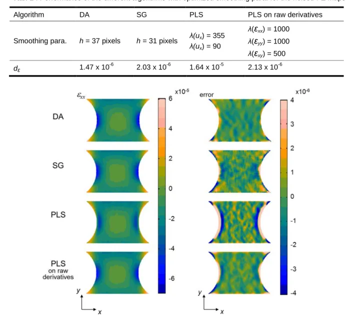
It can be observed that PLS works worse than both DA and SG. Indeed, the obtained average deviation in these conditions is an order of magnitude higher than the ones obtained for the two others algorithms. This counterbalances the conclusions of the previous section concerning the best performances of PLS. It appears especially that PLS does not manage to reconstruct correctly the edges of the circular notches, where the absolute deviation from the exact value of the strain is maximum (Fig. 4).
. Tab. 2 : Performance of the different algorithms with optimized smoothing para. for the noised FE maps
Algorithm DA SG PLS PLS on raw derivatives
Smoothing para. h = 37 pixels h = 31 pixels λ(ux) = 355
λ(ux) = 90 λ(
ε
xx) = 1000 λ(ε
yy) = 1000 λ(ε
xy) = 500 dε 1.47 x 10 -6 2.03 x 10⁻⁶ 1.64 x 10⁻⁵ 2.13 x 10⁻⁶Fig. 4 : Reconstructed
ε
xx and corresponding error maps for the different smoothing methods.However, when smoothing directly the raw derivatives as previously done for the noised analytical function, the reconstruction by PLS works more efficiently. Indeed, for an optimal set of λ's, the average deviation obtained is
of the same range as the one obtained with the two other algorithms.
In conclusion, it can be said that, if PLS is not the best procedure for this problem (possibly because the highest gradients are located on the edges of the maps which was not the case previously, with the analytical function), it shows results comparable with the ones produced by DA or SG when performing the derivation before the smoothing and remains the fastest method.
3.3. Smoothing of experimental kinematic maps
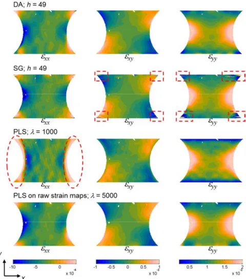
Finally, the smoothing procedure by PLS has been tested onto true experimental kinematic maps. The tensile test on a double notched specimen considered in the previous section has been examined. The displacement maps were obtained by the grid method [12]. The grid had a pitch of 100 µm leading to kinematic maps of 159 x 231 pixels2. The raw displacements fields have been processed by the different algorithms leading to strain maps represented in Fig. 5.
Fig. 5 : Experimental in-plane strain maps obtained on the double-notched tensile sample by applying
different smoothing procedures (size of the region of interest: 16 x 23 mm2).
In this figure, it can be clearly observed that both DA and PLS directly applied on raw strain maps lead to accurate maps that can be compared to the ones obtained on simulated data even if the experimental results show an asymmetry between the left and right sides due to some misalignment between the axis of the sample and the one of the testing device during the test (Fig. 4b). On the contrary, SG and PLS applied before deriving displacement maps do not work. Strain maps resulting from SG show a dithering effect probably due to the important influence of the edges (zones surrounded by dashed rectangles in Fig. 5). For the same reason, PLS applied before deriving displacement maps does not provide good results. This is especially the case for
ε
xx (zones surrounded by dashed ellipses in Fig. 5) that is here the most difficult map to reconstruct as the signal to noise ratio is the lowest (the x direction is not highly solicited in this test). So, for such a case, with high gradients on the edges and potentially low signal to noise ratio, it seems preferable to apply a point-to-point differentiation before smoothing by PLS rather than applying the smoothing and then differentiating the smoothed displacement maps: this produces results comparable with the ones of DA.4. CONCLUSION
In this paper, the possibility to use the penalized least squares smoothing procedure (PLS) as an alternative way to process kinematic full-field measurements has been addressed. At the end of this study, it can be asserted that PLS manages to produce valid strain maps from displacements measurements, with an accuracy comparable to
the techniques currently set up such as diffuse approximation (DA) or Savitzky-Golay smoothing filter (SG). Nevertheless, a precaution has to be taken: for kinematic measurements presenting high gradients on the edges of the studied region and showing low signal to noise ratio, it is highly preferable to apply PLS on raw strain fields, after a spatial derivation of displacement fields thanks to a simple point-to-point differences procedure.
Compared to other procedure such as DA or SG, PLS presents two main advantages:
– the computation time of the algorithm is independent of the value of the smoothing parameter and highly lower than both DA and SG;
– the h span parameter of DA and SG is an odd integer that gives only a discrete control of the amount of smoothing to apply; on the contrary, the smoothing parameter λ of PLS is a real continuous value.
Finally, PLS appears to be a robust alternative to currently applied smoothing techniques that can be preferentially selected whenever one has to process large maps that need a large amount of smoothing due to its high computation speed.
5. ACKNOWLEDGMENTS
The authors would like to thank Pr. Paul Eilers for some useful exchanges on the principles and developments of the penalized least squares algorithm. They also would like to thank Dr. Marco Rossi for providing the 2D Savitzky-Golay algorithm used in this study. Finally, they would like to thank their colleagues at Arts et Métiers ParisTech (especially, Mr. Alain Prévot, Ms. Virginie Jamar and Mr. Jeremy Blanks) for their help at different stages of the work.
6. REFERENCES
[1] Feissel, P.: From displacement to strain (Chap. 7). In Full-field measurements and identification in solid
mechanics, pages 191–221. John Wiley & Sons, 2013.
[2] Cordero, R.R., Molimard, J., Labbé, F. and Martínez, A.: Strain maps obtained by phase-shifting interferometry: an uncertainty analysis. Optics communications, 281(8):2195–2206, 2008.
[3] Moulart, R., Avril, S. and Pierron, F.: Identification of the through-thickness rigidities of a thick laminated composite tube. Composites Part A, 37(2):326–336, 2006.
[4] Avril, S., Feissel, P., Pierron, F. and Villon, P.: Comparison of two approaches for differentiating full-field data in solid mechanics. Measurement Science & Technology, 21(1):015703, 2010.
[5] Gorry, P.A.: General least-squares smoothing and differentiation by the convolution (Savitzky-Golay) method. Analytical Chemistry, 62:570–573, 1990.
[6] Bohlmann, G.: Ein Ausgleichungsproblem. In Nachrichten von der Gesellschaft der Wissenschaften zu Göttingen, Mathematisch-Physikalische Klasse, pages 260–271. 1899. (In German).
[7] Whittaker, E.T.: On a new method of graduation. Proceedings of the Edinburgh Mathematical Society, 41:63–75, 1923.
[8] Eilers, P. H. C.: A perfect smoother. Analytical Chemistry, 75:3631–3636, 2003.
[9] Garcia, D.: Robust smoothing of gridded data in one and higher dimensions with missing values.
Computational Statistics & Data Analysis, 54(4):1167–1178, 2010.
[10] Buckley, M. J.: Fast computation of discretized thin-plate smoothing spline for image data. Biometrika, 81(2):247–258, 1994.
[11] Avril, S., Pierron, F., Pannier, Y. and Rotinat, R.: Stress reconstruction and constitutive parameter identification in plane-stress elasto-plastic problems using surface measurements of deformation fields.
Experimental Mechanics, 48(4):403–419, 2008.
[12] Surrel, Y.: Moiré and grid methods: a signal-processing approach. In SPIE 2342, Interferometry ’94: