Mobilité et redistribution à long terme des éléments traces métalliques exogènes dans les sols : Application à des Luvisols pollués par 100 ans d'épandage d'eaux usées brutes dans la plaine de Pierrelaye

HAL Id: tel-00070810

https://pastel.archives-ouvertes.fr/tel-00070810

Submitted on 20 May 2006

HAL is a multi-disciplinary open access

archive for the deposit and dissemination of

sci-entific research documents, whether they are

pub-lished or not. The documents may come from

teaching and research institutions in France or

abroad, or from public or private research centers.

L’archive ouverte pluridisciplinaire HAL, est

destinée au dépôt et à la diffusion de documents

scientifiques de niveau recherche, publiés ou non,

émanant des établissements d’enseignement et de

recherche français ou étrangers, des laboratoires

publics ou privés.

traces métalliques exogènes dans les sols : Application à

des Luvisols pollués par 100 ans d’épandage d’eaux

usées brutes dans la plaine de Pierrelaye

Christelle Dere

To cite this version:

Christelle Dere. Mobilité et redistribution à long terme des éléments traces métalliques exogènes dans

les sols : Application à des Luvisols pollués par 100 ans d’épandage d’eaux usées brutes dans la plaine

de Pierrelaye. Sciences de la Terre. ENGREF (AgroParisTech), 2006. Français. �tel-00070810�

N° attribué par la bibliothèque

/__/__/__/__/__/__/__/__/__/__/

THESE

pour obtenir le grade de

Docteur de l'ENGREF

Spécialité : Sciences de l’Environnement

présentée par

Christelle Dère

Soutenue le

16 Mars 2006

à l’Institut National d’Agronomie Paris-Grignon

MOBILITE ET REDISTRIBUTION A LONG TERME DES ELEMENTS

TRACES METALLIQUES EXOGENES DANS LES SOLS

Application à des Luvisols pollués par 100 ans d’épandage d’eaux

usées brutes dans la plaine de Pierrelaye

devant le jury suivant :

M. Bruno FERRY

MC, ENGREF Nancy

Président du jury

MME. Catherine GRIMALDI CR, INRA Rennes

Rapporteur

MME. Catherine KELLER

PR, Université Aix-Marseille III Rapporteur

MME. Sabine HOUOT

DR, INRA Grignon

Examinatrice

M. Stephen NORTCLIFF

PR, University of Reading

Examinateur

M. Dominique KING

DR, INRA Orléans

Directeur de thèse

MME. Isabelle LAMY

CR, INRA Versailles

Encadrante

MME. Sophie CORNU

CR, INRA Orléans

Encadrante

Résumé

Afin d’identifier les principaux facteurs contrôlant la redistribution des éléments traces métalliques (ETM) exogènes dans le sol, nous avons utilisé une démarche intégrative à différentes échelles : constituants, solum et transect parcellaire. Cette démarche a été appliquée sur des Luvisols sableux de la région parisienne, fortement pollués par cent ans d’épandages massifs d’eaux usées brutes. Les ETM endogènes et les ETM exogènes ont été discriminés de manière à étudier spécifiquement le devenir des ETM amenés par les eaux usées brutes.

Dans l’horizon de labour, la distribution spatiale des ETM est fonction de la géométrie du système d’irrigation et de la topographie du terrain.

Dans le cas de Pb et de Cr, il n’y a pas d’exogène dans les horizons inférieurs (0.4-1m), constatation corroborée par leur spéciation, identique dans le sol contaminé et dans le sol témoin. Une estimation des flux d’ETM basée sur l’immobilité du chrome dans les sols, et sur la constance des rapports ETM/Cr dans les eaux d’épandage, indique que le plomb amené par les eaux usées brutes n’a pas migré. Les stocks d’exogène dans les horizons inférieurs montrent que par contre, Cu et Zn ont migré. Cu aurait été plus massivement mobilisé et exporté que Zn, ce dernier étant plus repiégé que Cu le long du profil. Les constituants et les mécanismes responsables du piégeage de Cu le long du solum n’ont pas été identifiés. Pour Zn, la recapture s’est faite principalement sur les oxyhydroxydes de fer et de manganèse. Les quantités de Zn fixées sont fonction du nombre de sites et de leur accessibilité, conditionnée par l’organisation des flux d’eau dans la parcelle.

Mots-clefs : eaux usées brutes, sols sableux, Luvisols, éléments traces métalliques exogènes, redistribution,

long-terme.

Abstract

In order to determine the main factors responsible for the distribution of exogenous trace metals (TM) in soil, we used an integrated multi-scale approach: constituents, solum and transect at the plot scale. This approach was applied to sandy Luvisols of Paris region that are highly polluted due to 100 years of raw waste water irrigation. Endogenous and exogenous TM contents were estimated in order to study the fate of those brought by the waste water.

In the ploughed surface horizon, the spatial distribution of TMs depends on the spatial design of the spreading system and on the plot topography.

No exogenous Pb and Cr are present in the deep horizons (0.4-1m). This result is coherent with the speciation of these elements which is similar in the polluted and in the unpolluted solum. TMs inputs to the soil were estimated considering that (i) the chromium is a poorly mobile element in soil and (ii) the TM/Cr ratios in waste water is poorly variable in time. This estimation showed that the Pb brought by the waste water to the soil was kept within the soil surface horizon. Stocks of exogenous Cu and Zn in the deep horizons showed that these elements migrated downward, Cu being more exported than Zn which has been retained more efficiently than Cu along the solum. Constituents and mechanisms responsible for Cu fixation along the solum were not identified. Zinc was mainly retained by iron and manganese oxides. The quantity of zinc retained was a function of the number of sites available and of their accessibility, which was in turn a function of the distribution of water fluxes within the plot.

Avant propos

Cette thèse est constituée de quatre articles soumis ou acceptés dans des revues internationales à comité de lecture. Certains ont été rédigés en français avant d’être traduits, et pour une plus grande simplicité de lecture, ce sont les versions françaises qui sont présentées dans ce manuscrit. L’intégralité des bibliographies des différents articles a été regroupée à la fin du document. Un cinquième article, en lien avec les travaux présentés mais toutefois un peu en marge du cœur de la thèse, est présenté en annexe.

Remerciements

Merci à l’INRA et à la région Ile-de-France d’avoir financé cette thèse, et merci à Isabelle Lamy, Sophie Cornu, et Dominique King de l’avoir encadrée.

Je remercie les multiples directeurs d’unité qui m’ont accueillie au sein de leur laboratoire : Claire Chenu, Daniel Tessier et Guy Richard. Merci Guy pour tes nombreuses relectures, toujours pertinentes et constructives.

Je remercie Catherine Keller et Catherine Grimaldi d’avoir accepté d’être rapporteurs de cette thèse, ainsi que Sabine Houot, Bruno Ferry et Stephen Nortcliff d’être membres du jury.

Je tiens à remercier tous les membres de mon comité de pilotage : Alain Bermond, Liliana Di Pietro, Bruno Ferry, Cyril Kao, Médard Thiry et Folkert van Oort.

Comme dans toute thèse, le nombre de personnes ayant pris part à ce travail est imposant. Qu’ils soient chercheurs, ingénieurs, techniciens, AJT, AGT, stagiaires, ou doctorants, beaucoup ont participé à cette thèse de par leurs conseils et/ou leur aide technique. Je remercie donc Folkert van Oort et Denis Baize pour leurs conseils en matière de prélèvements sur le terrain ; Anne Jaulin, pour m’avoir formée à l’utilisation du spectromètre d’absorption atomique et pour avoir activement participé à l’amélioration des déterminations analytiques ; Hocine Bourennane, dont la porte est toujours grande ouverte pour des explications en géostatistiques (et pour d’autres conversations plus légères) ; Catherine Pasquier, manipulatrice GPS efficace au bureau et sur le terrain ; Miguel Pernes pour les caractérisations DRX et ATD-ATG ; Loïc Prud’homme et Nicolas Chigot pour la détermination des propriétés hydrodynamiques du sol ; Marilyne Bruneau et Laetitia Citeau pour les analyses d’eaux gravitaires ; Cyril Kao et Cédric Chaumont, anciens collègues du Cemagref, pour leurs conseils en matière de suivi tensiométrique de plein champ ; Jocelyn Bonnet et Thibault Delannoy, mes deux stagiaires, petites mains dévouées au service de la science aux côtés de mes petites mains dévouées elles aussi à la science ; et aussi Christelle Fernandez, Eliane Huard, Nicole van Oort, Nelly Wolff, Sébastien Breuil, Pierre Courtemanche, Thomas Lagadec, Jean-Pierre Leydecker, Jean-Pierre Pétraud et Hervé Pouillot pour les différents services rendus sur le terrain, au laboratoire, ou au bureau.

Je n’oublie pas mes voisin(e)s de bureau (ou des bureaux voisins…) grâce auxquel(le)s le travail s’est effectué dans la bonne humeur : Anne, Arlène, Céline R et Céline CB (mes mères nourricières ;-) ), Florence,

Isabelle Le., Sophie C, Sophie L, Cédric, David, Gregory, Vincent C, et bien d’autres. Merci d’avoir fait du bureau un lieu de convivialité et de bonne humeur.

Je remercie les hôtes qui m’ont accueillie à titre gracieux avec beaucoup de gentillesse et de bienveillance durant mes périodes de transit entre les deux unités : Hocine et Nathalie, Cyril, et Mathieu.

Enfin, le meilleur pour la fin, je tiens à remercier tout particulièrement Sophie, dont l’énergie et la vivacité n’ont d’égales que sa ténacité et sa bonne humeur. Merci beaucoup pour ton soutien. Merci à Nicolas et à Eric, garants, déménageurs, mais surtout, amis sincères. Merci à Aurélie et Mathilde, les deux personnes avec lesquelles les conversations téléphoniques ne s’arrêtent que lorsque la batterie du téléphone est vide. Et pour finir, merci à Nelly et à Martin, dont l’amitié n’a de virtuelle que le nom.

Sommaire

Introduction ... 1

I. Problématique ... 1

II. Objectifs... 5

III. Contexte ... 6

III.1. L’utilisation des eaux usées... 6

III.2. Conséquences sur les sols ... 6

III.3. Conclusion... 7

Chapitre 1 : Présentation du site et stratégie d’échantillonnage ... 9

I. Historique de l’épandage des eaux usées en région parisienne ... 9

II. Le cas de la plaine de Pierrelaye... 9

III. Choix d’un site d’étude et stratégie d’échantillonnage... 10

Chapitre 2 : Distribution spatiale des ETM dans l’horizon de surface ... 13

I. Enhancing spatial estimates of metal pollutants in raw wastewater irrigated fields using a topsoil organic carbon map predicted from aerial photography... 13

I.1. Abstract ... 13

I.2. Introduction... 14

I.3. Material and methods ... 16

I.3.1. The site and the survey... 16

I.3.2. Kriging methods... 18

I.3.3. Validation criteria ... 20

I.4. Results and discussion ... 21

I.4.1. Summary statistics ... 21

I.4.2. Variography analysis and spatial prediction of TE by ordinary kriging ... 23

I.4.3. Trace elements (TE) spatial distributions estimated by cokriging ... 26

I.4.4. Trace elements (TE) mapping by collocated cokriging method... 28

I.4.5. Kriging TE using SOC map as an external drift ... 28

I.4.7. Sensitivity of KED and CC methods to the sampling density of the target

variables (TE)... 34

I.5. Conclusion ... 37

II. Recherche des facteurs responsables de la structure observée :... 38

III. Conclusion... 40

Chapitre 3 : Distribution des ETM en profondeur... 41

I. Etude à l’échelle des constituants : devenir à long terme des métaux exogènes dans un Luvisol sableux soumis à une irrigation massive par des eaux usées brutes ... 41

I.1. Résumé ... 41

I.2. Introduction... 42

I.3. Matériel et méthodes... 43

I.3.1. Les sols ... 43

I.3.2. Extraction et dosage des ETM ... 44

I.3.3. Spéciation des ETM exogènes ... 46

I.4. Résultats et discussion ... 46

I.4.1. Localisation des ETM dans le sol témoin ... 48

I.4.2. Spéciation des ETM exogènes dans le sol contaminé ... 49

I.5. Conclusion ... 57

II. Etude à l’échelle du solum : reconstitution des apports en éléments traces métalliques et bilan de leur migration dans un Luvisol sableux soumis à 100 ans d’irrigation massive par des eaux usées brutes.... 58

II.1. Résumé... 58

II.2. Introduction ... 58

II.3. Matériel et méthode ... 59

II.3.1. Description du site ... 59

II.3.2. Prélèvements de sol et analyses ... 60

II.3.3. Stocks d’ETM dus à la contamination ... 61

II.3.4. Reconstitution des apports d’ETM en surface ... 61

II.3.5. Calcul des incertitudes... 62

II.4. Résultats et discussion ... 62

II.4.2. Reconstitution des apports par le Cr ... 65

II.4.3. Discussion sur la mobilité relative des ETM au sein du solum ... 66

II.5. Conclusion ... 67

III. Etude à l’échelle de la toposéquence : déterminisme de la distribution tridimensionnelle du zinc dans un sol sableux suite à 100 ans d’épandage d’eaux usées brutes ... 68

III.1. Résumé ... 68

III.2. Introduction ... 68

III.3. Matériels et méthodes... 70

III.3.1. Présentation du site de Pierrelaye... 70

III.3.2. Les sols... 70

III.3.3. Stratégie d’échantillonnage ... 71

III.3.4. Estimation du fond pédo-géochimique naturel local ... 72

III.3.5. Analyses ... 73

III.4. Résultats et discussion... 73

III.4.1. Distribution horizontale... 73

III.4.2. Distribution verticale... 76

III.5. Conclusion... 83

Conclusion générale... 85

Perspectives ... 89

Bibliographie... 91

Introduction

I. Problématique

Les éléments traces sont les 68 éléments minéraux, constituants de la croûte terrestre, dont la concentration est, pour chacun d’eux, inférieure à 0,1% (Alloway, 1990c; Baize, 1997b). A eux tous, ils ne représentent que 0,6% du total des éléments. L’expression « élément trace métallique » (ETM) renvoie aux métaux (densité atomique supérieure à 6 g cm-3_{) présents à l’état de traces (cadmium, chrome, cuivre, nickel,} zinc, plomb…).

Les éléments traces métalliques dans les sols proviennent de différentes sources. Les uns, endogènes, sont hérités du matériau parental et redistribués dans les sols par les processus pédogénétiques. Ils constituent ce qu’on appelle le fond pédo-géochimique (Baize, 1997b). Les autres, exogènes, sont d’origine anthropiques (industries, épandages) ou naturelles (poussières, volcanisme) (Alloway, 1990c; Juste et Robert, 2000). Les principales sources d’ETM anthropiques sont les industries, l’urbanisme (chauffage, eaux usées, boues de station d’épuration), les transports (routiers, fluviaux), l’agriculture (fertilisants, herbicides, lisiers) (Alloway, 1990c). D’une manière générale, ces dernières décennies, la quantité d’ETM apportés aux sols a augmenté, entraînant des accumulations plus ou moins fortes de ces éléments (Alloway, 1990c; Juste et Robert, 2000; Lamy et al., 2005). On peut distinguer deux types de pollutions, des pollutions dites ponctuelles, généralement réduites à la parcelle et le plus souvent apportées par des effluents agricoles (lisiers), industriels ou urbains, et des pollutions plus diffuses, de taille régionales, dont le vecteur est le plus souvent atmosphérique (fumées de centrales thermiques, d’usines métallurgiques…).

Cette accumulation d’ETM dans le sol peut avoir des impacts néfastes sur l’environnement, avec, selon les cas, un risque de contamination des cultures, des eaux de surface ou des eaux souterraines. En effet, si la plupart de ces éléments sont nécessaires à la vie, à l’exception de Pb et de Cd pour lesquels on ne connaît pas à l’heure actuelle d’utilité biologique, ils sont toxiques à forte concentration (Mc Bride, 1994).

Une fois dans le sol, les ETM peuvent être prélevés par les végétaux, ou bien être redistribués dans le sol, en surface par l’érosion et le ruissellement, ou en profondeur, en migrant avec la solution du sol (Figure 1). Leur devenir dans l’environnement est très variable selon l’élément considéré.

ETM mobilisés

Percolation vers nappe temporaire superficielle

Prélèvement par les végétaux

Infiltration vers nappe souterraine profonde

Zone saturée (nappe temporaire superficielle) Zone non saturée

Ruissellement + Érosion

Apports exogènes en surface

ETM liés au sol Conditions physico-chimiques du milieu Apports latéraux Ruissellement + Érosion Drainage latéral ETM mobilisés

Percolation vers nappe temporaire superficielle

Prélèvement par les végétaux

Infiltration vers nappe souterraine profonde

Zone saturée (nappe temporaire superficielle) Zone non saturée

Ruissellement + Érosion Ruissellement + Érosion Apports exogènes en surface

ETM liés au sol Conditions physico-chimiques du milieu Apports latéraux Ruissellement + Érosion Drainage latéral

Figure 1 : Voies de transfert des éléments traces métalliques le long d’une toposéquence agricole ayant reçu des apports d’ETM en surface.

Concernant leur redistribution dans le sol, les ETM sont, en surface, redistribués latéralement par le labour et l’érosion diffuse (Korentajer et al., 1993; Zhao et al., 2001; Zang et al., 2003). A notre connaissance, seuls Yingming et Corey (1993) et Mc Grath et Lane (1989) ont estimé les quantités de métaux redistribués par le travail du sol. Yingming et Corey (1993) ont estimé que le travail du sol redistribuait, en une vingtaine d’années 15% à 20% des ETM apportés ; et Mc Grath et Lane (1989) estiment cette proportion à 21-28% sur une quarantaine d’années.

Pour ce qui est de la redistribution verticale, Yingming et Corey (1993) estiment que le transfert vertical représente 12% à 15% des apports alors que Mc Grath et Lane (1989) le chiffrent à environ 1%. Cette différence s’explique du fait du nombre de facteurs intervenant : spéciation, type d’éléments, organisation des flux...

En effet, le passage des ETM dans la solution du sol est contrôlé par la forme (i.e. spéciation) sous laquelle ils se trouvent dans la phase solide : échangeables, adsorbés, complexés à la surface des constituants du

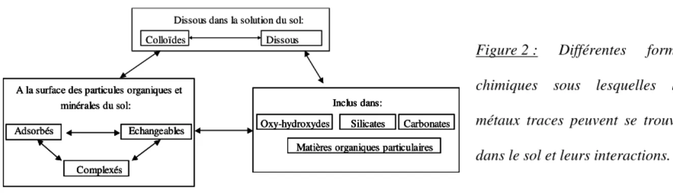
sol, ou co-précipités (Mc Bride, 1989; Kabata-Pendias, 1993). La matière organique, les carbonates, les argiles minéralogiques et les oxy-hydroxydes de fer et de manganèse sont les principaux constituants impliqués dans la rétention des ETM (Alloway, 1990b; Mc Bride, 1994; Harter et Naidu, 1995). Ainsi, la mobilité des ETM dans les sols des propriétés chimiques (Alloway, 1990b; Sager, 1992; Kabata-Pendias, 1993; Mc Bride, 1994; Charlatchka et Cambier, 2000) des horizons. Les interactions entre les différentes spéciations des ETM sont présentées Figure 2.

Figure 2 : Différentes formes chimiques sous lesquelles les métaux traces peuvent se trouver dans le sol et leurs interactions.

La spéciation dépend de la forme sous laquelle ont été amenés les ETM (Bataillard et al., 2003; Haiyan et Stuanes, 2003), de la nature et des proportions des constituants du sol (matière organique, oxy-hydroxydes, argiles) (Sager, 1992; Ledin et al., 1996), et des conditions du milieu (pH, Eh) (Alloway, 1995; Impellitteri et

al., 2001). De plus, les caractéristiques physico-chimiques du sol sont elles-mêmes influencées par les conditions

extérieures au milieu (cf Figure 3).

Figure 3 :

Facteurs influençant la spéciation des métaux dans le sol.

Localisation des éléments

traces dans les sols (en

solution, adsorbés, inclus dans les constituants du sol...)

Caractéristiques intrinsèques du sol: minéralogie, pH, matières organiques... Caractéristiques extrinsèques: climat, pratiques culturales, forme sous laquelle sont apportés les contaminants…

Composition de la solution du sol: pH, Eh, force ionique, présence de ligands…

Dissous dans la solution du sol: Dissous Colloïdes Inclus dans: Carbonates Silicates Oxy-hydroxydes

Matières organiques particulaires Adsorbés

Complexés

Echangeables A la surface des particules organiques et

minérales du sol:

Dissous dans la solution du sol: Dissous Colloïdes Inclus dans: Carbonates Silicates Oxy-hydroxydes

Matières organiques particulaires Inclus dans: Inclus dans:

Carbonates Silicates

Oxy-hydroxydes

Matières organiques particulaires Adsorbés

Complexés

Echangeables A la surface des particules organiques et

minérales du sol: Adsorbés

Complexés

Echangeables A la surface des particules organiques et

Une fois les ETM présents dans la solution du sol, leur migration sera fonction des propriétés physiques, notamment hydrodynamiques, des horizons (perméabilité, structure, (Camobreco et al., 1996; Simpson et al., 2004)) et de l’organisation des flux d’eau dans la parcelle (Calvet et Graffin, 1974; Martaud et Dinh, 1983; Bejat et al., 2000). Le sol étant organisé en une succession d’horizons aux caractéristiques pédologiques et hydrodynamiques différentes, les métaux vont être mobilisés (ou au contraire être à nouveau immobilisés) dans chacun des horizons lors du transfert de l’eau dans le sol.

Au final, on peut dire que la migration des ETM dans le sol dépend : • de l’élément considéré (Zn, Pb…)

• des propriétés chimiques et physiques (perméabilité, structure) des horizons • des caractéristiques physico-chimique de l’eau percolante (pH, Eh…)

• de la dynamique de l’eau transitant dans le sol et de l’organisation spatiale des flux d’eau

Tous ces paramètres doivent être pris en compte pour modéliser la mobilité, à long terme, de ces éléments persistants dans l’environnement.

Par conséquent, pour cerner au mieux la migration des ETM dans le sol, donc leur éventuel transfert vers les eaux souterraines, les eaux de surface, il faut prendre en compte deux échelles différentes :

• l’échelle microscopique des constituants (argile, oxy-hydroxydes, matières organiques…) pour comprendre la spéciation des ETM et leur mobilisation/immobilisation dans les différents horizons du sol. • l’échelle macroscopique (solum, parcelle…) pour comprendre la migration des ETM, en relation avec les transferts de soluté.

Cependant, les études menées jusqu’à présent présentent trois limites principales :

• le plus souvent, les études traitant de la migration des métaux considèrent que les flux sont principalement verticaux, et se limitent à du 1D vertical. Cette approche ne permet pas de prendre en compte d’éventuels transferts latéraux, alors qu’ils existent fréquemment dans les sols (Gaskin et al., 1989; Wilson et al., 1993; Shaw et al., 2001). Il serait donc intéressant d’évaluer le rôle de ces transferts dans la redistribution des ETM issus d’une contamination.

• la pollution d’un sol est souvent hétérogène du fait notamment du mode d’apport des polluants. On observe, dans l’horizon de surface, des variations à l’échelle métrique à pluri-métrique (Assadian et al., 1998; Sterckeman et al., 2000). Il est donc nécessaire d’étudier l’impact de la variabilité spatiale de la pollution sur la migration des ETM dans le sol. Sterckeman et al. (2000) ont observé, dans le cas d’une pollution minérale par des fumées d’usine, que la profondeur de migration du zinc était fonction de la contamination en surface. Pourtant, ce type de travaux reste rare et n’a jamais, à notre connaissance, été mené dans le cas de pollutions par des effluents organiques.

• le sol est un milieu hétérogène qui présente des propriétés chimiques et physiques variables à l’échelle métrique/plurimétrique (Gaston et al., 2001; Cichota et al., 2003; Giltrap et Hewitt, 2004; Mzuku et al., 2005). Là encore, peu d’auteurs ont étudié l’impact de ces variations verticales et latérales sur la migration et la rétention des ETM dans le sol.

Aussi il semble nécessaire, pour une meilleure évaluation des risques liés à la migration d’ETM dans les sols contaminés, de procéder à des études multi-échelles. Ce type d’études permet d’identifier, à chaque échelle, les principaux facteurs mis en jeu dans la mobilisation et la migration des ETM, et de déterminer si ces facteurs sont les mêmes quelque soit l’échelle considérée.

II. Objectifs

L’objectif de ce travail est donc d’étudier la redistribution, à long terme, des ETM dans une parcelle fortement contaminée par les ETM. Dans un premier temps, l’étude a porté sur la distribution de la pollution en surface, puis, dans un deuxième temps, sur la redistribution des ETM en profondeur, en fonction des propriétés physico-chimiques des horizons et des constituants du sol. Le travail a été mené selon une logique d’échelles emboîtées constituantsÆ solum Æ parcelle.

Le site d’étude est un site contaminé par des eaux usées brutes. Le chapitre 1 est consacré à la présentation du site d’étude et au choix d’une stratégie d’échantillonnage. Le chapitre 2 présente l’organisation spatiale de la pollution dans l’horizon de surface. Le chapitre 3 porte sur la redistribution des ETM en profondeur, à l’échelle des constituants tout d’abord, puis du solum, et enfin du transect. Pour finir, la conclusion

rassemble les résultats marquants de ce travail, et les propositions de recherche souhaitées pour conforter et poursuivre ces travaux.

III. Contexte

III.1. L’utilisation des eaux usées

L’épandage d’eaux usées brutes en agriculture permet d’irriguer les cultures, d’épurer l’eau et de recycler des éléments nutritifs, le tout de manière économique. A la fin du 19ème_{, cette méthode avait souvent été} mise en place autour des grandes villes pour éliminer les quantités croissantes d’eaux usées liées à l’urbanisation de la population (Streck et Richter, 1997a; Filip et al., 1999; Vedry et al., 2001). Il s’agissait alors d’un moyen de « traitement » des eaux usées à peu de frais. Avec la construction des usines de traitement d’eaux usées, ce procédé est/a été progressivement abandonné. Toutefois, il est encore utilisé dans les zones arides (dans lesquelles l’usage de l’eau doit être optimisé) et dans les régions où les moyens d’épuration sont insuffisants comparé aux volumes à traiter (Assadian et al., 1999; Jiries et al., 2002; Yadav et al., 2002).

III.2. Conséquences sur les sols

Le problème le plus souvent observé est la salinisation des sols et un colmatage de la porosité dû à l’accumulation des particules organique et à la dispersion des argiles sous l’effet de la salinisation (Vinten et al., 1983; Shahalam et al., 1998; Tarchitzky et al., 1999; Agassi et al., 2003; Viviani et Iovino, 2004). Il en résulte une diminution de la conductivité hydraulique de l’horizon de surface, ce qui augmente le ruissellement et diminue l’infiltration.

Par ailleurs, même si certains auteurs rapportent que l’irrigation par des eaux usées n’a pas entraîné d’accumulation significative d’ETM dans l’horizon de surface (Cebula, 1980; Ramirez-Fuentes et al., 2002), il est fait constat de nombreux cas de contamination par les métaux (Schirado et al., 1986; Flores et al., 1997; Schalscha et Ahumada, 1998; Jiries et al., 2002), certains auteurs rapportant en outre une migration vers la profondeur (Flores et al., 1997; Streck et Richter, 1997a). Ce type de pollution amené par des eaux usées est particulier car il amène de la matière organique, des sels et des flux d’eaux en plus ou moins grande quantité, et

de façon pas forcément homogène si on compare à une pollution diffuse par dépôt atmosphérique par exemple. L’introduction dans un sol de carbone organique n’est pas anodin, en raison des aspects ambivalents des relations matières organiques-métaux, aboutissant soit à un stockage soit à un relargage de métaux, suivant la nature de la matière organique et les conditions physico-chimiques du sol (Karapanagiotis et al., 1991; Lamy et

al., 1994; Harter et Naidu, 1995; Christensen et al., 1996; Merritt, 2003). De plus, la présence de sel peut

favoriser la migration des ETM dans le sol (Boyle et Fuller, 1987).

III.3. Conclusion

L’irrigation par eaux usées brutes est une pratique qui a encore cours dans de nombreux pays, soit du fait de l’aridité du climat, soit du fait du manque de station de traitement. Dans ce contexte, l’étude d’un site pollué de longue date par l’épandage d’eaux usées offre un recul intéressant aux pays qui utilisent encore ce procédé, et qui doivent gérer au mieux le risque de pollution de leurs sols et de leurs cultures (Carr, 2004).

Chapitre 1 : Présentation du site et stratégie d’échantillonnage

I. Historique de l’épandage des eaux usées en région parisienne

Au milieu du 19ème siècle, le principe d’épuration des effluents urbains de la ville de Paris par le sol a émergé à la fois comme solution au problème de la pollution grandissante de la Seine et comme solution au déficit des matières organiques, révélé par les agronomes, dont souffraient les terres agricoles. Malgré de vives polémiques faisant s’affronter agronomes, urbanistes, hygiénistes, agriculteurs ou riverains, le principe du recyclage des eaux usées par épandage sur les terres agricoles prévalut finalement sur le rejet des effluents en rivière. Suite aux plaintes de riverains concernés par les épandages d’eaux usées de la ville de Paris, une enquête d’utilité publique fut lancée en 1876 pour recenser les arguments des plaignants et étudier la salubrité du procédé d’épandage. Les travaux d’irrigation par les eaux usées brutes furent déclarés d’utilité publique en 1894. Le système mis en place visait à répondre à quatre objectifs : débarrasser la ville de Paris de ses immondices, éviter la perte d’éléments fertilisants, limiter la pollution grandissante de la seine, récupérer l’eau épurée par le sol pour la distribuer aux parisiens. En 1894, on épandait 30 millions de m3 _{d’eau sur une surface de 900 ha (soit une} lame d’eau moyenne de 3,3 m) (D'Arcimoles et al., 2000). Aux environs de 1910, on compte 220 millions de m3 épandus sur 5500 hectares de terres irriguées par l’épandage des effluents parisiens répartis de part et d’autre de la Seine, et recevant en moyenne 40000 m3 _{par hectare et par an (soit une lame d’eau moyenne de 4 m)} (D'Arcimoles et al., 2000). Devant l’intensification des épandages, les controverses ne cesseront de s’amplifier jusqu’en 1930, date de la construction de la première station d’épuration à Achères.

II. Le cas de la plaine de Pierrelaye

La plaine de Pierrelaye est une plaine agricole qui se situe dans la banlieue nord-ouest de Paris. L’irrigation par les eaux usées y a duré de 1899 à 2002, date à laquelle l’utilisation d’eau clarifloculée a été imposée sur le site (Vedry et al., 2001). A l’origine, c’était une plaine entièrement maraîchère, puis la partie nord fut convertie en maïsiculture dans les années 70, et la partie sud en 2000, suite à l’interdiction faite par le Conseil Supérieur d’Hygiène de France de vendre de la production maraîchère de ce site (Baize et al., 2002).

Les polluants métalliques apportés au cours d'un siècle d'irrigation par les eaux usées de la Ville de Paris sur des sols agricoles, ou par toute autre source dans un tel contexte péri-urbain, ont été progressivement incorporés dans l'horizon superficiel, soit directement avec l'infiltration de l'eau, soit mécaniquement suite aux labours annuels et retournement des croûtes de particules solides séchées en surface. Cette incorporation progressive a abouti à un horizon de labour fortement anthropisé, dont la contamination n’est pas influencée par la pédologie.

III. Choix d’un site d’étude et stratégie d’échantillonnage

Le nord de la plaine se trouve sous de grandes étendues de monoculture de maïs, alors que le sud est découpé en petit parcellaire anciennement sous maraîchage. Deux types de sol majoritaires dans la plaine sont les Calcisols et les Luvisols (Isambert et Baize, 2001) (figure 1).

Afin de nous affranchir de la variabilité liée aux pratiques culturales et aux changements de végétation, nous avons choisi de travailler dans la zone traditionnellement sous monoculture de maïs. L’îlot d’irrigation (zone délimitée par un réseau de bouches d’irrigation) y constitue l’unité d’organisation principale (figure 1).

Luvisols

Calcisols

Ilot d’irrigation

étudié

0 100 m

Luvisols

Calcisols

Ilot d’irrigation

étudié

0 100 m Bouches d’irrigation Bouches d’irrigation

Figure 1 : Pédologie de l’îlot étudié (à gauche) et position des bouches d’irrigation autour de l’îlot (à droite).

Pour l’étude de la distribution de la pollution en surface, 87 échantillons de l’horizon de labour ont été prélevés de manière aléatoire au sein d’une grille à maille carrée (Figure 2).

Figure 2 : Plan d’échantillonnage de l’horizon labouré au sein de l’îlot.

L’étude des redistributions en profondeur a été menée dans les Luvisols. Dans ce type de sol, les propriétés physico-chimiques des horizons sont très contrastées, ce qui laisse présager des comportements très différents des ETM selon les horizons. Trois transects ont été échantillonnés, deux orientés dans le sens de la pente, et un perpendiculairement à la pente (Figure 3).

Figure 3 : Plan d’échantillonnage des transects.

Enfin, les bilans de flux d’une part, et l’étude de la redistribution des ETM au sein des constituants d’autres part, ont été réalisés sur un des solums échantillonné précédemment (Y1), choisi pour sa situation en position plane supposée limiter les phénomènes d’érosion en surface.

Prélèvements Courbes isohypses (m) X1 Y1 Y2 Y3 Y4 X3 X4 Z3

Axe des transects Prélèvements Courbes isohypses (m)

X1 Y1 Y2 Y3 Y4 X3 X4 Z3

Chapitre 2 : Distribution spatiale des ETM dans l’horizon de surface

Dans ce chapitre, nous avons étudié l’organisation spatiale de la pollution dans l’horizon de surface. Les apports d’eaux usées brutes étant arrêtés, cet horizon peut être considéré comme la source de polluants pour les horizons inférieurs. Lors d’une étude préliminaire, nous avions mis en évidence, sur une trentaine de points, une corrélation forte (coefficient de corrélation de Pearson compris entre 0.86 et 0.95) entre les teneurs en matière organique et les teneurs en ETM, pour la partie Nord de la plaine. Nous avons donc décidé d’utiliser cette corrélation pour améliorer l’estimation des teneurs en ETM au sein de l’îlot. Concrètement, il s’agissait d’utiliser le carbone organique comme un traceur de la contamination, et de prévoir les teneurs en ETM à partir de données sur les teneurs en carbone organique. C’est l’objet de l’article (accepté pour publication dans la revue Science of the Total Environment) présenté au début de ce chapitre. Dans une deuxième partie du chapitre, nous avons cherché à identifier les facteurs à l’origine de la distribution spatiale observée.

I. Enhancing spatial estimates of metal pollutants in raw wastewater irrigated fields using a topsoil

organic carbon map predicted from aerial photography

H. Bourennane (1)_{, Ch. Dère} (2)_{, I. Lamy} (2)_{, S. Cornu} (1)_{, D. Baize} (1)_{, F. van Oort} (2) _{D. King} (1)

(1) _{INRA, Unité de Science du Sol, BP 20619 Ardon, 45166 Olivet Cedex, France} (2) _{INRA, Unité de Science du Sol, RD 10, 78026 Versailles Cedex, France}

I.1. Abstract

Various approaches have been used to estimate metal pollutant element (TE) contents at unsampled locations in a 15 ha contaminated site located in the plain of Pierrelaye-Bessancourt (about 24 km Northwest of Paris). 87 samples of soil plough layer were randomly sampled at each mesh of a regular square grid over the whole study area and the total contents of Cd, Cr, Cu, Ni, Pb, and Zn were measured. A first set of 50 measurements, randomly selected from the 87 samples, was used for the prediction and another set of 37 measurements was kept for the validation. Topsoil organic carbon contents (SOC) were measured at 75 sites with 50 measurements sharing the same locations as TE. An aerial photography of the study area showing bare

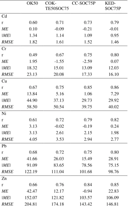
soils was selected for relating brightness intensities and SOC. Mapping procedures used were ordinary kriging (OK), cokriging (COK), collocated cokriging (CC) and kriging with external drift (KED). SOC maps used as exhaustively sampled information in KED and CC of TE were obtained by KED and CC procedures, respectively, accounting for 75 SOC measurements and the brightness intensities of numerical counts provided by the visible bands of the aerial photograph bare soils. Consequently, for each TE four maps were generated, two maps resulting from KED and CC procedures (KED-SOC75P, CC-SOC75P), another one was provided by standard cokriging (COK-TE50SOC75) accounting for TE prediction set plus 75 SOC measurements and the last one corresponds to that estimated by ordinary kriging from only prediction set measurements (OK50). Three indices, (1) the mean prediction error (ME) and the mean absolute prediction error (|ME|), (2) the root mean square error (RMSE), and (3) the relative improvement (RI) of accuracy, as well as residuals analysis, were computed from the validation set (observed data) and predicted values. On the 37 test data, the results showed that the more accurate predictions were systematically those obtained by kriging accounting for SOC map predicted by KED from 75 SOC measurements and brightness values of the aerial photo (KED-SOC75P) followed closely by CC-SOC75P procedure, except for Cu and Zn where CC-SOC75P appeared to be slightly more accurate than KED-SOC75P. In regard to the RI of accuracy between prediction methods, the results confirmed once for all the benefit of accounting for SOC data set plus the exhaustively sampled information provided by the aerial photography regardless the considered TE. Nevertheless, for Cd, Pb, and Zn, the RI of accuracy was less than 20 % between the two most accurate methods (KED-SOC75P and CC-SOC75P) and standard cokriging in which the information provided by the aerial photography is ignored when mapping.

The sensitivity of KED-SOC75P and CC-SOC75P approaches to the sampling density of the target variables (TE) was assessed using ten random subsets of different sizes (25 and 33 observations) drawn from a prediction set that includes 50 data. Results have shown that the TE estimates by KED-SOC75P and CC-SOC75P approaches using only 25 TE samples were much more accurate than the estimates performed by OK50 and COK-TE50SOC75 approaches that use the whole samples of the prediction set. Moreover, the RI of accuracy was reduced by less than 15 % if the original sampling density was reduced by a third.

I.2. Introduction

Accurate characterization of the spatial distribution of pollutants in contaminated soils is essential for risk assessment and soil remediation. Predictions are often required as well as a quantification of the

uncertainties inherent in spatial prediction. However, costs involved with measuring trace element (TE) concentrations exhaustively, in order to account for wide variability of pollutant distribution at the field scale, are prohibitive. Thus, very often trace elements are sparsely sampled at the field scale and interpolation algorithms such as ordinary kriging (OK) commonly used for spatial estimates performs poorly for mapping the spatial variation (Goovaerts, 1999). Consequently, other geostatistical techniques have been used to improve the accuracy of spatial prediction of target variables, especially those based on easy to obtain auxiliary variables (e.g. Bourennane et al., 1996; Zhang et al., 1997; Chaplot et al., 2000; Mueller and Pierce, 2003; Bourennane and King, 2003).

The present study is part of a research program (Baize et al., 2002), which assesses the risks of metal transfer into the food chain, metal migration towards depth and risks of contamination of groundwater, and feasibility of phytoremediation of polluted soils of the 1500 ha wide plain of Pierrelaye-Bessancourt (France). Consequently, accurate maps of TE spatial distribution are required for a proper risk assessment and soil remediation projects.

Preliminary soil survey of the whole 1500 ha irrigation area of Pierrelaye-Bessancourt combined with geochemical analytical work revealed strong correlation between organic carbon contents and metal pollutants (Baize et al., 2002). Correlation was different for areas under distinct major land use and management (Lamy et al., 2005), ascribed to historic of irrigation practices and the intensity of additional urban and organic residue amendments. Strong correlation of organic carbon and metal pollutants was found to be mainly due to their simultaneous introduction in the soils via irrigation of soils with raw wastewater from the Paris region. Such close relationships between organic carbon and total metal element concentrations in soils amended with organic waste residues were also stressed in literature (Karapanagiotis et al., 1991; McBride, 1994; Alloway 1995; McBride et al., 1997). Additional detailed study on metal distribution in a representative soil profile of the study area gave evidence for distinct metal associations with phosphate mineral, particulate organic matter, clay mineral and iron oxides, but the far most dominant metal localization was found with amorphous “urban organic matter intimately mixed with very fine carbonate crystals, occurring as organic coatings around sand skeleton grains (van Oort et al., 2005)”.

This study aims to examine the potential value of aerial photographs to infer topsoil organic carbon content variation in a raw wastewater contaminated area. Indeed as revealed in other studies over the study area and more generally stressed in the literature, TE concentrations in topsoil horizons are often related to topsoil organic carbon ‘SOC’. Moreover, it is well known that brightness intensities of numerical counts provided by the

visible bands of aerial photographs bare soils could be explained by SOC content variations (Krishnan et al., 1980; Escadafal et al., 1988 & 1989; Fernandez et al., 1988; Chen et al., 2000).

Thus, the basic idea is to accurately map SOC over the 15 ha study area using an aerial photography of bare soils and SOC measurements, and then to examine the impact of accounting for SOC map previously predicted in enhancing spatial estimates of TE.

For the purposes above, collocated cokriging (CC) and kriging with an external drift (KED) methods (Wackernagel, 1995; Goovaerts, 1997; Deutsch and Journel 1998; Chilès and Delfiner, 1999) were used to predict TE accounting for SOC maps predicted by CC and KED, respectively, using numerical counts of exhaustively sampled information provided by an aerial photography of study area bare soils and 75 SOC measurements.

Obviously, the more straightforward way to estimate a target variable from much more sampled variable is to perform cokriging (COK). Thus our target variables (TE), sampled at 50 locations, were also estimated by cokriging using TE samples and 75 SOC measurements.

Moreover, to examine the performances of CC, KED and COK methods over the commonly used method for spatial estimates, namely ordinary kriging (OK) method, the spatial distribution of total contents in Cd, Cr, Cu, Ni, Pb, and Zn obtained by the mentioned methods above were compared to these resulting from OK. Finally, the sensitivity of the more accurate method in our study regarding the sampling density of the target variables (TE) was examined using different sample densities.

As several methods are compared, the objective way of making the comparisons is to validate the predictions against actual observations that had not been used in obtaining the predictions. Accordingly, the data set was split up into two subsets: the first set (prediction set) was used for inference and prediction, and the second set (validation set) for the purpose of validation.

I.3. Material and methods

I.3.1. The site and the survey

The study area (one irrigation plot in the plain of Pierrelaye-Bessancourt) is located about 24 km Northwest of Paris covering a surface of 15 ha. According to Baize et al., (2002), wastewater has been used for

garden market irrigation between 1899 and 2000 over the study area. Moreover, soils were amended with urban sludge and smut compost in the middle 60’s.

Topsoil samples (plough layer) were randomly taken on each mesh of a regular square grid over the study area. Thus, the total contents of Cd, Cr, Cu, Ni, Pb, and Zn were measured after HF + HClO4 + HCl digestion at 87 locations. 37 sites randomly selected were kept aside for validation (the validation set). Therefore, the 50 remainder sites formed the prediction set. Topsoil organic carbon contents (SOC) were measured at 75 sites (Fig. 1a). Among these SOC 75 sites, 50 measurements shared the same locations as TE. SOC and TE (prediction set) were thus measured on the same soil samples for the 50 shared locations. Finally, the brightness values of an aerial photography (Fig. 1b) of the bare soils, taken in April 1996, were assigned to these locations (75 sites). Thus, based on the geographic co-ordinates of the soil observations in the field, each soil sample hwas assigned related with the mean brightness value of 10 cells around the sample location. Furthermore, dry topsoil conditions, previous to the photo acquirement, were the main criterion to select the aerial photography among the large number of aerial photographs available for the study area. The brightness values of the selected aerial photography are thus an indicator of SOC variations due to the wastewater spreading. In any case the brightness values in our study neither reflect the topsoil wet over the study area nor variations of topsoil texture which is sandy over the whole study area.

I.3.2. Kriging methods

The mapping procedures included the ordinary kriging, cokriging, collocated cokriging and kriging with external drift. The theory underlying these methods has been described in several geostatistical textbooks (e.g. Wackernagel, 1995; Goovaerts, 1997; Deutsch and Journel, 1998; Chilès and Delfiner, 1999; Webster and Oliver, 2000). Here, we describe the major steps for these procedures.

I.3.2.1. Ordinary kriging (OK)

In this section, we recall the forms of the predictor. We assume that the target variable,

Z

( )

x

is a random variable at all positions

x

in the region and that the particular set of values in the region is just one realization of it,

z

( )

x

.

In the ordinary kriging, the predictor of

z(

x

₀

)

for an unsampled location

x

₀ is:

),

(

)

(

1 0 α α α

x

x

w

z

z

n OK

∑

= ∗

₌

(1)

where

w

_α, are weights associated with the n sampling points. The weights sum to unity, a condition that ensures

a zero error in expectation.

I.3.2.2. Cokriging (COK)

Let there be V auxiliary variables,

V =

1

,

2

,

...,

N

,

and let us denote the one we wish to predict as z: this will usually have been less densely sampled than the others. Thus, the total set of variables consists of

1

+

V

attributes. The ordinary cokriging estimator is a linear combination of weights l

w

_α with data from

different variables located at sample points

(

x

α

)

in the neighborhood of a point

x

0. In the case of a single

auxiliary variable

(

V

=

1

)

, as in our study, the ordinary cokriging estimator of

z

(

x

₀

)

for an unsampled location

x

₀ is written:

)

(

)

(

)

(

2 ₂ 2 2 1 1 1 1 1 1 0 * α α α α α α

x

x

x

=

∑

+

∑

′

′

= =

V

w

z

w

z

n n COK (2)

where the

w

_α1’s are the weights applied to the

n

₁z samples and the

w′

_α2 are the weights applied to the

n

₂V

samples.

In the framework of a joint intrinsic hypothesis we wish to estimate a particular variable of a set of (

V

+

1

) variables on the basis of an estimation error which should be nil on average. This condition is satisfied by choosing weights which sum up to one for the target variable and which have a zero sum for the auxiliary variables.

.

otherwise

0

if

1

1







=

∑

=

z

=

l

w

l n l α α

I.3.2.3. Collocated cokriging (CC)

Cokriging requires a joint model for the matrix of semivariance functions including the Z semivariance

)

(h

Z

γ

, the U semivariance

γ

_U

(h

)

, and the cross Z-U semivariance

γ

_ZU

(h

)

.

Consequently, the inference becomes extremely demanding in terms of data and the subsequent joint modeling is particularly tedious. We state however that algorithms exist to fit automatically a linear model of coregionalization (e.g. Goulard, 1989; Goulard and Voltz, 1992) to a set of direct and cross semivariograms. In any case, for mainly the reason mentioned above, the cokriging has not been extensively used in practice. Algorithms such as kriging with an external drift, which can only account for auxiliary variable that is available at all primary data locations and interpolation grid nodes, and collocated cokriging, beyond its own shortcoming, have been developed to shortcut the tedious inference and modeling process required by cokriging.

Indeed, a reduced form of cokriging called collocated cokriging (Xu et al., 1992) exists and consists of retaining only the collocated auxiliary variable

U

(

x

₀

)

, provided that it is available at all locations being estimated. The

cokriging estimator (2) is written:

)

(

)

(

)

(

₀ 1 0 * 1 1

x

x

x

w

Z

w

U

Z

n CC

=

∑

+

′

= α α α , (3)

with the single constraint that all weights must sum to one and the auxiliary variable must be rescaled to the mean of the primary variable to ensure unbiased estimation.

The corresponding cokriging system requires the inference and modeling of only the Z semivariance

)

(h

Z

approximation (Zhu and Journel, 1993; Almeida and Journel, 1994; Goovaerts, 1997) through the following model:

γ

ZU

(

h

)

=

B

.

γ

Z

(

h

),

∀

h

(4)

where

B

=

C

_U

(

0

)

/

C

_Z

(

0

)

.

ρ

_ZU

(

0

)

,

C

_Z

(

0

)

,

C

_U

(

0

)

are variances of Z and U, and

ρ

_ZU

(

0

)

is a linear correlation coefficient of collocated data.

The main assumption underlying the Markov-type model is that which assume that the experimental semivariogram of the primary variable is proportional to the cross semivariogram. Thus, it is important to check whether such proportionality actually holds true.

I.3.2.4. Kriging with external drift (KED)

KED is a particular case of universal kriging. It allows the prediction a variable Z, known only at small set of points of the study area, through another variable s, exhaustively known in the same area. We choose to model Z with a random function Z(x) and s as a deterministic variable s(x). The two quantities are assumed to be linearly related, i.e. it is assumed that the expected value of Z(x) is equal to s(x) up to a constant a0 and a

coefficient b1.

Thus, KED consists in incorporating into the kriging system supplementary universality conditions about one or several external drift variables

s

_i

(

x

),

i

=

1

,

2,

..,

M

measured exhaustively in the spatial domain. The functions

s

i

(x

)

need to be known at all locations

x

α of the samples

Z

( )

x

as well as at nodes of the estimation grid.

In this method, we assume linear relationships between the variable of interest and the auxiliary variables. This assumption is very important in the prediction using KED method. Thus, if a non-linear function better describes the relationships between the two variables, this function should first be used to transform the data of the auxiliary variable. The transformed data could then be used as external drift.

I.3.3. Validation criteria

The performances of mapping procedures were assessed using several criteria. Therefore, the accuracy of the mapping procedures was assessed by computing (1) histograms of residuals resulting from each mapping

procedure and scatter plots of actual versus predicted values at each validation site, (2) the mean prediction error (ME) as well as the mean absolute prediction error (|ME|), and (3) the root mean square error of prediction (RMSE) which are defined as follows

[

]

∑

[

]

∑

= =

−

=

−

=

n i i i n i i i

Z

Z

n

ME

Z

Z

n

ME

1 1

)

(

)

(

1

and

,

)

(

)

(

1

* *

x

x

x

x

(5)

[

]

0.5 1 2 *

₍

₎

)

(

1













−

=

∑

= n i i i

Z

Z

n

RMSE

x

x

(6)

ME criterion was used to check the conditional bias property which consist in assuming that prediction

errors cancel out leading to an unbiased estimator over the whole range of values. Furthermore, |ME| criterion was measured for more relevant comparisons which avoid the fact that the negative and positive biases tend to cancel each other.

The RMSE criterion is a measure of accuracy of the various prediction methods. RMSE value should be as small as possible for accurate prediction.

Finally, the relative improvement (RI) of accuracy was calculated by

100

)

(

×

−

=

R E R

RMSE

RMSE

RMSE

RI

(7)

where RMSER and RMSEE are the root mean square errors for the reference and evaluated methods, respectively.

Thus, if RI is positive, the accuracy of the evaluated method is superior to the reference and conversely (Zhang et al., 1992).

I.4. Results and discussion

I.4.1. Summary statistics

Table 1 reports the descriptive statistics of the different data sets. The sample statistics of sets P and V differed except for Ni. This illustrates the importance of sampling variation which not only might influence the statistics of the different data sets but also the results of the validation study. Nevertheless, the mean values of sets P and V were statistically similar for all variables. The marginal distributions were approximately symmetric to moderately skewed (Cd). The brightness values of an aerial photography assigned to sample locations exhibit

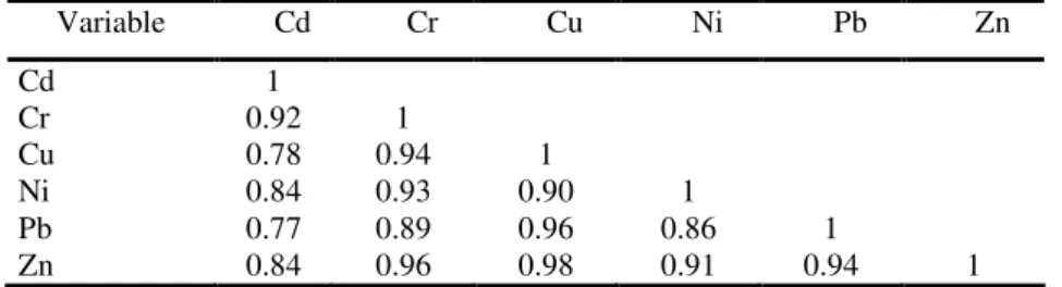
symmetrical distribution and lower CV. Topsoil organic carbon contents (SOC) are much higher than usual SOC contents in sandy agricultural soils. This clearly illustrates the long term use of raw wastewater for market garden practices in the study area leading to an important accumulation of exogenous organic matter. Scatter plots of SOC versus TE as well as linear correlation coefficient values (Fig. 2a) reveal high correlations between topsoil organic carbon contents and trace element concentrations, confirming the findings by Baize et al., 2002 and Lamy et al., 2005. Moreover, TE are strongly correlated (Table 2), stressing their simultaneous input originating from raw wastewater irrigation. Finally, the scatter plot of SOC versus brightness value (Fig. 2b) indicates that the assumption of a linear relationship between SOC and brightness value is not unreasonable.

Table 1: Descriptive statistics of the different data sets (P: prediction set; V: validation set)

Variable n Unit Min Max Mean S.D. CV (%) Skewness

Cd P 50 mg kg-1 _{1.58 11.51 3.98 2.07 52 1.53} V 37 mg kg-1 _{1.80 12.64 3.94 2.20 56 1.98} Cr P 50 mg kg-1 _{41.82 147.58 76.03 26.35 35 0.94} V 37 mg kg-1 _{47.88 150.47 77.06 25.92 34 1.06} Cu P 50 mg kg-1 _{66.88 319.33 173.40 64.72 37 0.43} V 37 mg kg-1 91.66 339.54 185.33 71.89 39 0.69 Ni P 50 mg kg-1 _{11.56 29.37 18.97 4.71 25 0.47} V 37 mg kg-1 _{12.80 31.69 19.31 4.72 24 0.96} Pb P 50 mg kg-1 _{117.73 648.66 321.58 131.24 41 0.64} V 37 mg kg-1 _{138.75 757.39 358.62 151.24 42 0.65} Zn P 50 mg kg-1 297.48 1241.21 684.07 233.07 34 0.55 V 37 mg kg-1 _{372.20 1294.30 722.63 251.01 35 0.79} SOC P 75 g kg-1 _{10.40 41.83 21.48 7.66 36 0.62} Value* _{75 109.21 125.90 116.79 4.56 4 0.14}

*Brightness values at sample locations obtained from an aerial photography

Table 2: Linear correlation matrix for six TE in the topsoil (values based on prediction set: n = 50)

Variable Cd Cr Cu Ni Pb Zn Cd 1 Cr 0.92 1 Cu 0.78 0.94 1 Ni 0.84 0.93 0.90 1 Pb 0.77 0.89 0.96 0.86 1 Zn 0.84 0.96 0.98 0.91 0.94 1

10 15 20 25 30 35 40 SOC (g kg-1₎ 0 250 500 750 1000 1250 1500 Z n (m g k g -1) 10 15 20 25 30 35 40 SOC (g kg-1₎ 0 3 6 9 12 15 C d (m g k g -1) 10 15 20 25 30 35 40 SOC (g kg-1₎ 0 50 100 150 200 C r (m g k g -1) 10 15 20 25 30 35 40 SOC (g kg-1₎ 10 15 20 25 30 35 N i (m g k g -1) 10 15 20 25 30 35 40 SOC (g kg-1₎ 0 100 200 300 400 C u (m g k g -1) r = 0.83 r = 0.94 r = 0.95 r = 0.92 r = 0.94 r = 0.96 (a)

Figure 2: (a) Scattergrams of topsoil organic carbon (SOC) versus trace elements (TE) and values of linear correlation coefficients based on prediction set: n = 50; (b) Scattergram of topsoil organic carbon (SOC) versus brightness intensity value of bare soils and linear correlation coefficient value (b) r = -0.47 n = 75 10 15 20 25 30 35 40 SOC (g kg-1₎ 100 200 300 400 500 600 700 P b (m g k g -1) 10 15 20 25 30 35 40 45 SOC (g kg-1₎ 105 110 115 120 125 130 B ri g h tne s s in te n s it y 10 15 20 25 30 35 40 SOC (g kg-1₎ 0 250 500 750 1000 1250 1500 Z n (m g k g -1) 10 15 20 25 30 35 40 SOC (g kg-1₎ 0 250 500 750 1000 1250 1500 Z n (m g k g -1) 10 15 20 25 30 35 40 SOC (g kg-1₎ 0 3 6 9 12 15 C d (m g k g -1) 10 15 20 25 30 35 40 SOC (g kg-1₎ 0 3 6 9 12 15 C d (m g k g -1) 10 15 20 25 30 35 40 SOC (g kg-1₎ 0 50 100 150 200 C r (m g k g -1) 10 15 20 25 30 35 40 SOC (g kg-1₎ 0 50 100 150 200 C r (m g k g -1) 10 15 20 25 30 35 40 SOC (g kg-1₎ 10 15 20 25 30 35 N i (m g k g -1) 10 15 20 25 30 35 40 SOC (g kg-1₎ 10 15 20 25 30 35 N i (m g k g -1) 10 15 20 25 30 35 40 SOC (g kg-1₎ 0 100 200 300 400 C u (m g k g -1) 10 15 20 25 30 35 40 SOC (g kg-1₎ 0 100 200 300 400 C u (m g k g -1) r = 0.83 r = 0.94 r = 0.95 r = 0.92 r = 0.94 r = 0.96 (a)

Figure 2: (a) Scattergrams of topsoil organic carbon (SOC) versus trace elements (TE) and values of linear correlation coefficients based on prediction set: n = 50; (b) Scattergram of topsoil organic carbon (SOC) versus brightness intensity value of bare soils and linear correlation coefficient value (b) r = -0.47 n = 75 10 15 20 25 30 35 40 SOC (g kg-1₎ 100 200 300 400 500 600 700 P b (m g k g -1) 10 15 20 25 30 35 40 SOC (g kg-1₎ 100 200 300 400 500 600 700 P b (m g k g -1) 10 15 20 25 30 35 40 45 SOC (g kg-1₎ 105 110 115 120 125 130 B ri g h tne s s in te n s it y 10 15 20 25 30 35 40 45 SOC (g kg-1₎ 105 110 115 120 125 130 B ri g h tne s s in te n s it y

I.4.2. Variography analysis and spatial prediction of TE by ordinary kriging

The spatial autocorrelation (Fig. 3) was quite strong for all TE. To these experimental variograms were fitted nested models (pure nugget plus a spherical model and power model). The coefficients of the fitted functions are given in Table 3. In an attempt to validate the variogram models, the cross validation was used on the original data (prediction set). Every known point was estimated by using a neighborhood around it, but not itself. Having made such calculations, the mean error defined by

[

]

R

n

i

z

i

z

i n

=

∗

−

=

∑

1

1

( )

x

( )

x

,

(8)

should be close to zero, and the ratio of the mean squared error to the kriging variance

,

)

(

)

(

)

(

1

1 2 2

∑

= ∗

























−

=

n i k i i i R

z

z

n

S

x

x

x

σ

(9)

0 100 200 300 0 1 2 3 4 5 6 S emi va ri an ce (m g kg -1) 2 00 100 200 300 25 0 50 0 75 0 10 00 00 100 200 300 15 00 30 00 45 00 60 00 0 100 200 300 Distance (m) 0 10 20 30 S emi va ri an ce (m g kg -1) 2 0 100 200 300 Distance (m) 0 80 00 16 00 0 24 00 0 0 100 200 300 Distance (m) 0 30 00 0 60 00 0 90 00 0 Cd Cr Cu Ni Pb Zn 0 100 200 300 0 1 2 3 4 5 6 S emi va ri an ce (m g kg -1) 2 00 100 200 300 25 0 50 0 75 0 10 00 00 100 200 300 15 00 30 00 45 00 60 00 0 100 200 300 Distance (m) 0 10 20 30 S emi va ri an ce (m g kg -1) 2 0 100 200 300 Distance (m) 0 80 00 16 00 0 24 00 0 0 100 200 300 Distance (m) 0 30 00 0 60 00 0 90 00 0 Cd Cr Cu Ni Pb Zn

Figure 3: Experimental variograms (dots) and their theoretical models fit (solid lines)

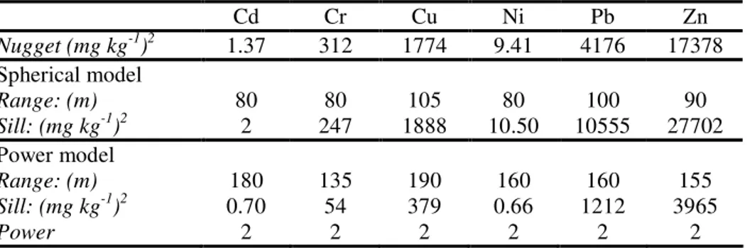
Table 3 : Coefficient of the theoretical variogram functions fitted to the experimental variograms of six TE.

Cd Cr Cu Ni Pb Zn Nugget (mg kg-1)2 1.37 312 1774 9.41 4176 17378 Spherical model Range: (m) 80 80 105 80 100 90 Sill: (mg kg-1)2 2 247 1888 10.50 10555 27702 Power model Range: (m) 180 135 190 160 160 155 Sill: (mg kg-1)2 0.70 54 379 0.66 1212 3965 Power 2 2 2 2 2 2

Table 4: Cross validation results in moving neighborhood for TE data: statistics based on prediction set (n = 50)

Variables R 2 R

S

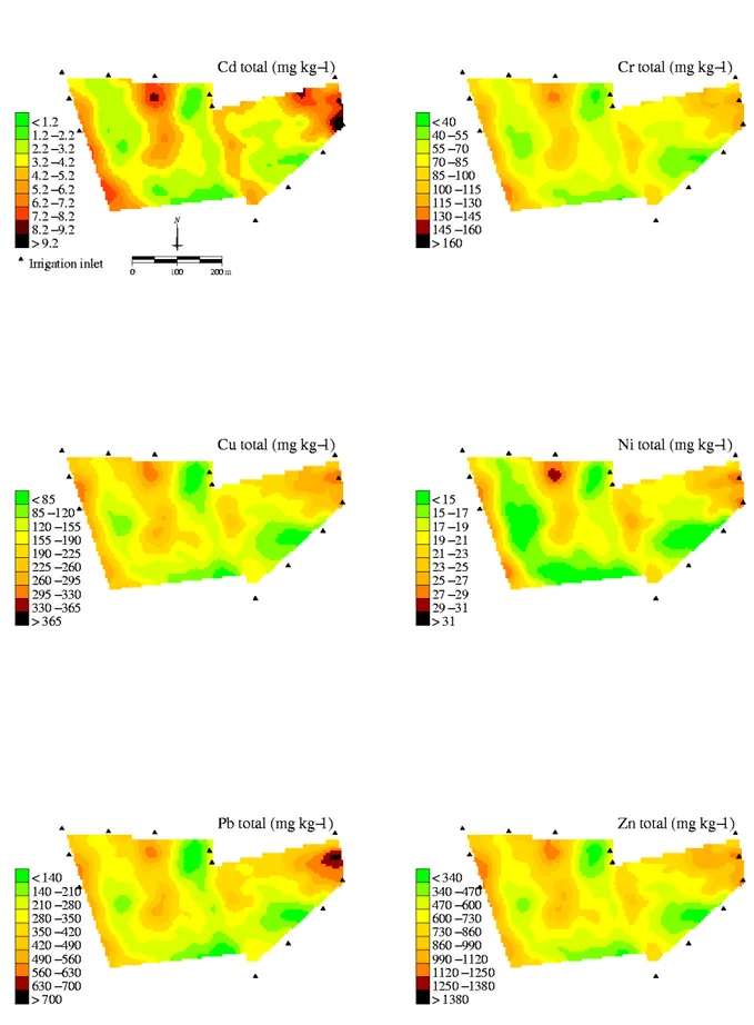
Cd -0.076 1.152 Cr -0.547 1.109 Cu -0.466 0.980 Ni -0.078 1.034 Pb 0.325 1.020 Zn -0.521 1.052

The results of the calculations (Table 4) using a moving neighborhood are revealing. They show that mean errors (between -0.547 and 0.325) are close to zero, and the variance ratios (between 0.980 and 1.152) are close to 1. Thus, using the fitted variogram functions and the kriging equation system, TE were estimated (Fig. 4) over the 15 ha study area from only punctual measurements corresponding to each TE, respectively. The smooth variations (Fig. 4) could be attributed to the nugget effect and the smoothing inherent in the estimator. Furthermore, smooth aspects of maps (Fig. 4) are very likely due to the short range of the semivariograms and the low sampling intensity of the prediction set. The resulting maps (Fig. 4) showed globally similar patterns and they reveal that to TE concentrations are higher near to irrigation inlets except for two irrigation inlets at the middle part of the study area and one in the south east part of the maps. Actually, some irrigation inlets are not functional. Finally, spatial distribution of TE concentrations is partly related (results not shown) to flow paths estimated from digital elevation model (DEM) even if slope intensity is very gentle over the study area.

Figure 4: Maps of six elements (TE) estimated by ordinary kriging.

I.4.3. Trace elements (TE) spatial distributions estimated by cokriging

As shown (Fig. 2a) TE are strongly related to SOC and less densely sampled (Fig. 1a) than SOC. Thus, we can use our knowledge of the spatial relations between TE and SOC to estimate the target variables (TE) from data on them plus those of SOC which we regard as auxiliary variable. The linear model of coregionalization was fitted (Fig. 5) to the cross-variograms of SOC with TE. The degree of coregionalization was assessed by the closeness of the cross-variogram to the ‘hull of perfect correlation’ (Wackernagel, 1995), which comprises the lines of perfect positive and negative correlation. Thus, the lines of the fitted models (Fig. 5) showed positive coregionalizations, as did the correlation coefficients and were closer to the hull (dashed lines in Fig. 5) of perfect correlation, indicating stronger spatial relations between SOC and selected TE. Thus, using the fitted model of coregionalization and the cokriging equation system, trace elements were estimated by cokriging (Fig. 6) using 50 TE measurements and 75 SOC measurements as auxiliary variable. The cokriged TE maps (Fig. 6) showed similar pattern than those resulting from ordinary kriging (Fig. 4) with more detail and less smoothness than the kriged TE maps. Moreover, the cokriging estimation variances (values not shown) are smaller than those of kriging estimates especially at the points where SOC values were known.

0 100 200 300 Distance (m) -1 000 0 10 00 0 100 200 300 Distance (m) -1 200 0 12 00 24 00 0 100 200 300 Distance (m) -3 0 -1 5 0 15 30 45 C ro ss -v ar io gr am (m g kg -1) 2 0 100 200 300 -2 0 -1 0 0 10 20 C ro ss -v ar io gr am (m g kg -1) 2 0 100 200 300 -1 50 0 15 0 30 0 0 100 200 300 -6 00 -3 00 0 30 0 60 0

Cd x SOC Cr x SOC Cu x SOC

Ni x SOC Pb x SOC Zn x SOC

0 100 200 300 Distance (m) -1 000 0 10 00 0 100 200 300 Distance (m) -1 200 0 12 00 24 00 0 100 200 300 Distance (m) -3 0 -1 5 0 15 30 45 C ro ss -v ar io gr am (m g kg -1) 2 0 100 200 300 -2 0 -1 0 0 10 20 C ro ss -v ar io gr am (m g kg -1) 2 0 100 200 300 -1 50 0 15 0 30 0 0 100 200 300 -6 00 -3 00 0 30 0 60 0

Cd x SOC Cr x SOC Cu x SOC

Ni x SOC Pb x SOC Zn x SOC

Figure 5: Cross-variograms of TE versus SOC. The experimental values are plotted as points and the solid lines are of the model of coregionalization. The dashed lines in graphs are the hulls of perfect correlation.

Figure 6: Maps of six trace elements (TE) estimated by cokriging using 50 TE measurements and 75 soil organic carbon (SOC) measurements.