Any correspondence concerning this service should be sent to the repository administrator:
staff-oatao@listes-diff.inp-toulouse.fr
O
pen
A
rchive
T
oulouse
A
rchive
O
uverte (
OATAO
)
OATAO is an open access repository that collects the work of Toulouse researchers and makes it freely available over the web where possible.
This is an author-deposited version published in: http://oatao.univ-toulouse.fr/ Eprints ID: 24603
To cite this version: Herpin, Sophie and Perret, Laurent and Mathis, Romain and Tanguy, Christian and Lasserre, Jean-Jacques
Application of Laser Doppler Anemometry to estimate turbulent power spectra inside an urban canopy. (2018) In: 19th International Symposium
on the Application of Laser and Imaging Techniques to Fluid Mechanics, 16 July 2018 - 19 July 2018 (LISBON, Portugal)
Application of Laser Doppler Anemometry to estimate turbulent power spectra
inside an urban canopy
Sophie Herpin1,4, Laurent Perret1, Romain Mathis2, Christian Tanguy3, Jean-Jacques Lasserre3 1: LHEEA, Ecole Centrale Nantes, UMR CNRS 6598, Ecole Centrale de Nantes, B.P. 92101,
F-44321 NANTES Cedex 3, France
2: Institut de Mécanique des Fluides de Toulouse, IMFT, Université de Toulouse, CNRS - Toulouse, France 3 : DANTEC Dynamics SAS 8 rue Gutenberg, ZI de la Butte 91620 Nozay, France
4 : EPHor, AGROCAMPUS OUEST, 2 rue André Le Nôtre 49045 ANGERS cedex, France * Correspondent author: sophie.herpin@agrocampus-ouest.fr
Keywords: Laser Doppler Anemometry, urban canopy, turbulence, power spectral density
ABSTRACT
In the present contribution, we propose to make use of Laser Doppler Anemometry to investigate the dynamics of the flow inside an urban canopy immersed into a thick turbulent boundary layer. Previous studies dedicated to such flows (Castro et al. 2006; Reynolds and Castro 2008) have focused the core of their analysis on the roughness sublayer region or on the inertial region. In contrast, the region below the canopy interface have received little attention so far, and only mean velocity or Reynolds stresses data can be found in the literature. Indeed, getting access to the dynamics of the flow inside the canopy represents a real experimental challenge: the flow is turbulent, 3-dimensionnal, and due to the tight clearance, only non-intrusive laser-based techniques such as LDA or PIV can be used. In this contribution, for the first time, a spectral analysis of the flow is carried out inside the canopy region. This is made possible thanks to very thorough LDA measurements as well as the use of advanced post-processing algorithm to compute temporal power spectra. Indeed, LDA measurement yields non-equidistantly spaced data points, and standard FFT algorithms cannot be used. A detailed comparison of various algorithms is undertaken, and a slight improvement is proposed to reduce the impact of measurement noise. Finally, the power spectra inside the canopy are analyzed and the main implications on the flow dynamics are discussed.
1. Introduction
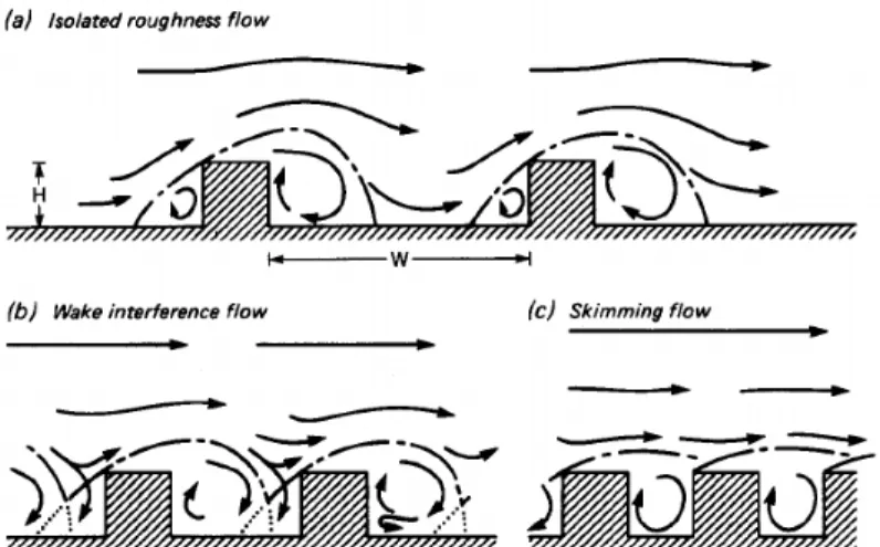
—•Ž›œ•Š—•’—•1Š•–˜œ™‘Ž›’Œ1••˜ œ1’—1ž›‹Š—1Š›ŽŠœ is of primary importance in the context of urban densification of the worldwide population. Despite the very large range of building size, shape, or spatial arrangement in real-life built areas, the simplified canopy consisting of a regular array of cubes is now widely accepted as a canonical representation. From the aerodynamics point of view, Oke (1988) and Grimmond and Oke (1999) identified three flow regimes depending on the packing area density of the urban roughness (see Fig. 1): the isolated roughness flow in which the
organization of the flow is very similar to single-cube flow, the wake interference flow, and the skimming flow.
The first insights into the dynamics of the flow over dense urban canopies have been given by Castro et al. (2006), using Hot-Wire Anemometry (HWA) and Laser Doppler Anemometry (LDA) to measure the flow above and below the canopy interface respectively, at 4 measurement stations. They investigated a staggered array of cubes with a tw¨ density pertaining to the wake-interference regime, with a boundary layer to building height ratio of A ŠLyäv and a Reynolds number of AEL A — K N {zr (where — is the friction velocity, K the kinematic viscosity, ˆ1 •‘Ž1 ‹˜ž—•Š›¢1 •Š¢Ž›1 •‘’Œ”—Žœœ1 Š—•1 ‘1 •‘Ž1 ‹ž’••’—•1 ‘Ž’•‘•). Mean flow and Reynolds stresses wall-normal profiles were obtained inside the canopy. Temporal power spectra were analyzed above the canopy using HWA, but not inside the canopy.
Following these first successful measurements, and in order to retrieve spatial information within the canopy, Castro's group made use of both PIV and LDA in a staggered-cube 25% canopy with A ŠLsuäw with AENvur (Reynolds and Castro 2008). The LDA measurements were performed at consistent locations with their previous study. The 2D-2C PIV was realized in a streamwise/wall-normal šæœ plane centered on a streamwise row of cubes, and going down to the wall. The mean statistics of the flow were extracted and showed a very good agreement between PIV and LDA. A detailed two-point spatial correlation and quadrant analysis was then undertaken using PIV data. In contrast to smooth-wall data, it was found that sweeps are dominant close the wall within the canopy region. The spatial auto-correlation of the streamwise velocity component was finally analyzed.
Some limitations arise from the above-mentioned studies: the datasets are obtained at moderate Reynolds number (ŠELŠ — K Ð >vurâsrzr?; as well as small boundary layer thickness to cube
height ratio (A Š Ð >yävâsuäw?). This is due to the limited thickness of the boundary layer in conventional wind-tunnels. This does not enable a full reproduction of the very large scale motions in the outer region of real atmospheric flows, and therefore of the complex inner/outer interactions with the canopy flow. Moreover, the dynamics of the flow, which requires advanced post-processing of time-resolved data, was not realized inside the canopy region.
In the present contribution, we propose to investigate an urban canopy flow in conditions which are representative of real atmospheric flows using Laser Doppler Anemometry. A detailed comparison of various algorithms to compute power spectra is undertaken, and a slight improvement is proposed to reduce the impact of measurement noise. Finally the results are analyzed to gain more understanding about the dynamics of the flow.
2. Experimental Design and Methods 2.1 Experimental setup
The experimental dataset is acquired in the LHEEA atmospheric wind-tunnel at Ecole Centrale de Nantes. After appropriate conditioning with spires and fence, the boundary layer develops over a 24 m long floor, fully covered with an urban canopy model consisting of a regular, staggered array of 50 mm high cubes with a packing area density of 25% (see Fig. 2 and Fig. 3). An extensive characterization of the flow above the canopy can be found in Perret et al. (2018). The main characteristics are summarized in Table 1. The flow benefits from a high Reynolds number (ŠELsvtr and AELuturr, with h the building height and Å the boundary layer thickness) and a boundary layer thickness-to-building height ratio A Š Lttäy which are relevant for real urban-like environments. The boundary layer is representative of the atmospheric surface layer in neutral conditions at the scale sãtrr.
Ue (m/s) A:•; u* (m/s) A + h+ A Š z0/h d/h
5.78 1.134 0.4278 32300 1420 22.7 0.11 0.59
Table 1 : Main characteristics of the flow (z0: aerodynamic roughness length ; d: displacement thickness) The dynamics of the flow inside the canopy was recorded using a two-component laser doppler anemometry system from Dantec Dynamics (model FlowExplorer DPSS), operating in backward scattering mode. A schematic representation of the experimental setup is shown in Fig. 2. In this study, the streamwise, spanwise and wall-normal directions are denoted šá ›á œá respectively and
associated with velocity components —á ˜á ™. The measurement volume size expressed in wall units is šEL ›ELtäz and œELtz, or as a fraction of the cube height is š ŠL › ŠLrärrt and œ ŠLrärt. An extensive description of the LDA measurements can be found in Herpin et al. (2018) and the main points are summarized below.
Fig. 3 : Position of the LDA measurement points
The streamwise and spanwise velocity components have been measured at seven streamwise/spanwise positions inside the canopy, chosen to be representative of the canopy pattern: P1, P2, P3 as defined by Castro's group (Castro et al. 2006; Reynolds and Castro 2008), plus three additional points A, B, C, D to study the flow dynamics in the vicinity of a cube (see Fig.
3). These points are measured at three heights inside the canopy: h/4, h/2, and h. In order to validate the LDA data and power spectra, three additional wall-normal positions have been measured above the canopy with both LDA (at œLsätwŠá sävwŠ ƒ•† wŠ at point noted E) and HWA
(at z=1.5h and z=5h, same position but shifted 4h downstream to avoid any blockage effect on the LDA measurements). The HWA probes are single-wire probes with a wire diameter of 5 ÍP and a wire length of 1.25 mm. This length is comparable with the height of the LDA measurement volume, resulting in a similar spatial resolution. The HWA signal is sampled twice: firstly, with an independent acquisition system with regular sampling at 10kHz; secondly, at the LDA sampling rate (the HWA analog signal being fed as an analog input to the LDA system). These two different samplings of the HWA signal will be used in this contribution to compare the performance of different power spectra algorithms.
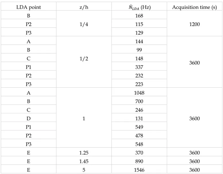
The mean LDA particle rate 06Žº depends on the position of the measurement point and naturally decreases when going down to the wall (see Table 2).
LDA point z/h 06Žº (Hz) Acquisition time (s)
B 1/4 168 1200 P2 115 P3 129 A 1/2 144 3600 B 99 C 148 P1 337 P2 232 P3 223 A 1 1048 3600 B 700 C 246 D 131 P1 549 P2 478 P3 548 E 1.25 370 3600 E 1.45 890 3600 E 5 1546 3600
In any case, it is between 1 to 3 orders of magnitude higher than the expected characteristics frequencies of the flow, which are of the order of fouter § 5Hz in the outer region (based on the boundary layer thickness Å and the free-stream velocity Ue) and finner § 8Hz in the inner region (based on the building height h and the friction velocity u*). It ensures an appropriate time resolution of the flow dynamics.
2.2 Power spectra Algorithms
The estimation of power spectra density, which is of primary importance to investigate the energy distribution inside turbulent flows, is not trivial on LDA data because the irregular sampling does not allow for the use of standard FFT algorithms. A number of algorithms to compute Power Spectra on LDA data exist and have been reviewed in Benedict et al. (2000) and can be classified in three categories:
x Direct Estimations Methods (Velte et al. 2014), with a Direct Fourier Transform computed directly on the randomly sampled signal (without the use of FFT).
x Time Quantization Methods such as Slotting Technique (Mayo Jr et al. 1974),where particle arrival time are grouped into time-slots of fixed duration; the auto-correlation function is then computed and transformed into the spectral domain using an FFT algorithm.
x Interpolation Methods, where the original signal is interpolated into a continuous signal with a zeroth order scheme (Sample and Hold) or a first-order scheme (Linear Interpolation), and then re-sampled at a fixed datarate enabling the use of standard FFT algorithms.
From the literature, it can be said that the Direct Estimation Method (Velte et al. 2014) provides the most reliable results. It preserves the integrity of the original LDA signal, giving a bias-free and low variance estimator. However, the impossibility to run FFT algorithm results in very high computational times, that can become prohibitive for large datasets.
In contrast, the interpolation techniques are much more time-efficient, but introduce a significant bias in the estimation of the power spectra, due to the transfer function of the interpolation scheme. The Sample and Hold interpolation is more popular than the linear interpolation or other higher-order schemes, the main reason being that, thanks to the work by Adrian and Yao (1986), the Sample and Hold transfer function can be expressed as an analytic function:
5èáÌÁ:ñ; L s
s E ñ6 066H5è:ñ; E têè 6 6
6
067I (1)
where Su is the power spectra of the streamwise velocity, 5èáÌÁis the estimate of the power spectra using the Sample and Hold algorithm, Ú is the circular frequency, 06 is the mean datarate of the LDA signal, Ôu is the variance of the input signal, and 6 is the Taylor micro-scale. Thus, the Sample and Hold Estimator behaves as a low-pass filter (first term before parenthesis in equation 1) with added step noise (second term inside parenthesis in equation 1). It is of interest to note that both the filtering effect and noise of the estimate are minimized as the LDA datarate 06 increases. The existence of this analytical formula allows to derive a correction of the Sample and Hold transfer function. This refinement of the Sample and Hold algorithm have been proposed by Nobach et al. (Nobach et al. 1998) with a correction factor that can be applied to the auto-correlation function, yielding a bias-free estimator of the power spectra in the spectral domain:
4:G; L :t? E s;4:G; F ?:4:G F s; E 4:G E s;; avec ? L Ø
7¿6
:5?Ø7¿6;. (2)
This refined Sample and Hold algorithm yields a much better estimate of the power spectra with a lower bias error. However, as pointed out by Nobach et al. (1998) the corrected estimator shows an increased variance than the uncorrected one; it also requires more CPU time than the basic algorithm.
Finally, the Slotting Technique (Mayo Jr et al. 1974) is often considered as the reference technique to estimate LDA power spectra, with minimal transformation of the original LDA signal and a better computational efficiency than the Direct Estimation Method. In that sense, it can be considered as a compromise between the Interpolation Techniques and the Direct Method. The Slotting Technique yields a faithful estimate of the power spectra, but the variance of this estimator is very large at high frequencies. A refinement of the Slotting technique, namely the Fuzzy Slotting technique, was implemented by Van Maanen et al. (1999) and is a mean to temper this variance.
In the literature, these algorithms were classically validated using simulation datasets or experimental dataset within an axisymmetric jet, taking hot-wire anemometry (HWA) as reference data. In the present contribution, we carry out a comparison of these algorithms in the framework of our urban turbulent boundary layer flow. The analysis is carried out in the roughness sublayer
(œLsäwŠ) and inertial layer region (œLwŠ), where the HWA measurements can be used as a reference. The subsequent LDA algorithms were investigated:
x basic Sample and Hold or linear interpolation
x refined Sample and Hold, with correction (Nobach et al. 1998) x fuzzy Slotting (Van Maanen et al. 1999)
x Arrival Time Quantization (Nobach 2016)
The Python library available on the Signal and Data processing Nambis website from Nobach and co-workers (http://ldvproc.nambis.de/index.html) was used to implement these LDA power spectra algorithms. These algorithms were assessed against a reference power spectrum obtained from HWA measurements in the same flow, with a regular sampling at sr• œ and standard FFT algorithm.
At first, a study of the influence of the LDA irregular sampling and power spectra algorithm is carried out, independently of the influence of the measurement technique itself: the power spectrum from the HW probe at œLsäwŠ, digitized with regular sampling at sr• œ, is compared with the power spectra from the same HW analog signal, but digitized by the LDA system with irregular sampling at a mean datarate of 223Hz (during acquisition of P3 at z=h/2): see Fig. 4.
Fig. 4 : Power spectra of streamwise velocity component in standard form (left) and in pre-multiplied form (right) measured at z=1.5h with HWA, obtained with different sampling and power spectra algorithms. The reference power spectra (black) obtained with a regular sampling at 10kHz and a standard Welch FFT algorithm, is compared with the power spectra of the same analog signal with LDA irregular sampling at a mean datarate of 223Hz. Various algorithms are compared for the computation of spectra with LDA sampling
As it can be seen, the Slotting and Arrival Time Quantization produce spectra with a high variance, while the Sample and Hold and linear interpolation have a low-pass filtering effect. These is consistent with previous results in the literature summarized above. The Refined Sample and Hold algorithm appears to yield a quite faithful estimate with moderate variance.
In a second study, a comparison of the global influence of the measurement techniques (HWA and LDA) and post-processing algorithms is undertaken. In Fig. 5, the spectra from the HW probe at z=5h, sampled at 10kHz, is compared with the spectra measured with the LDA system at z=5h, with LDA sampling at a mean datarate of 1546Hz. As it can be seen, the estimation of the LDA spectrum is less affected by the choice of power spectra algorithm than on figure Fig. 4, thanks to the higher mean datarate of LDA data (1546Hz). But, deeper inside the canopy region where the datarates are lower, a stronger influence is expected.
On the basis of the review and benchmark carried out on the different algorithms to compute power spectra on LDA data, we decided to use the refined Sample and Hold algorithm for the flow analysis of our database. Indeed, this algorithm seems to provide the best trade-off between faithfulness, CPU efficiency, and low variance.
A further improvement of the refined Sample and Hold Algorithm is proposed in the present contribution. It can be of interest for all studies involving the computation of autocorrelations and
Fig. 5: Comparison of the Power spectra of streamwise velocity measured at z=5h with a hot-wire probe at 10 kHz and with a LDA system at a mean datarate of 1546 Hz. The reference HW power spectra (black) is compared with the LDA power spectra with various spectra algorithms
power spectra on a real experimental signal, including measurement noise. If we assume that the measurement noise of LDA is white, then it affects all frequencies of the power spectra. In contrast, in the temporal domain, the auto-correlation function is only affected at 0 time lag, where the noise correlates with itself, inducing an over-estimation of Ruu(0) :
4èè:r; L êè6E Ýè6 (3)
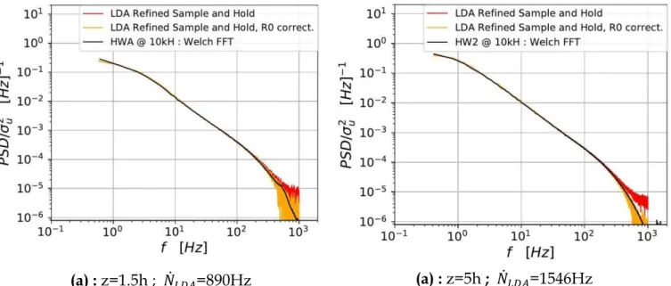
where Æu is the measurement noise and Ôu is the variance of the input signal. This influence of noise can be visualized on the auto-correlation function by a sharp peak at Ruu(0). In order to reduce the contamination of the power spectra by noise, it is possible to correct Ruu(0) using an extrapolation from neighboring points, before applying the Fourier Transform. After careful inspection of the shape of auto-correlation function in the neighborhood of Ruu(0), the extrapolation function is chosen as the osculating parabola of the auto-correlation function ˆ‘” œ RŠ, and as a decreasing exponential for œOŠ. The resulting LDA spectra, with the Refined Sample and Hold algorithm, with and without Ruu(0) noise correction is shown in Fig. 6, and compared with the reference HWA spectrum at sr œ. As it can be seen, for both algorithms the inertial range is successfully resolved by LDA. The correction of Ruu(0) reduces the effect of noise at high frequencies and gives further access to part of the dissipative range.
(a) : z=1.5h ; 06Žº=890Hz (a) : z=5h ; 06Žº=1546Hz
Fig. 6 : Comparison of the Power Spectral Density of streamwise velocity component obtained from HWA at 10 kHz and a standard FFT algorithm, with the PSD from LDA and a Refined Sample and Hold algorithm, with and without noise correction on Ruu(0)
3. Results
Mean velocity as well as Reynolds stresses results can be found in Herpin et al. (2018) and have shown good agreement with data in the literature (Castro et al. 2006; Coceal et al. 2006; Rivet 2014; Blackman and Perret 2016).
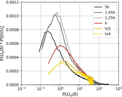
In this contribution, we focus on power spectra results computed using the Refined Sample and Hold with noise correction. An extract of the results is shown below: the PSD of the streamwise velocity component obtained from the LDA data is shown in the pre-multiplied form in Fig. 7 for point P2 at the different heights inside the canopy: œLŠ vá œLŠ tá œLŠ, in outer-scaling (color lines). We added the power spectral density measured above the canopy interface at point E, in the roughness sub-layer at œLsätwŠá œLsävw, and œLwŠ (grey and black lines).
The power spectrum is found to have the highest level (more energy) in the roughness sub-layer at œLsätwŠ ƒ•† œLsävwŠ, followed by the inertial region (œLwŠ), and finally by the canopy (less energy). Using a Taylor hypothesis in the inertial layer above the canopy, the size of the large-scale motions given by the frequency of the main peak of energy can be retrieved. It is of the order of uäuA, as classically observed in turbulent wall-bounded flows. Inside the canopy, the energy is the highest at the canopy interface (œLŠ) and then decreases with decreasing wall-normal distance, down to œLŠ t. In the vicinity of the wall (œLŠ t and Š v), the level of energy is low and stable
Fig. 7 : Wall-normal evolution of the pre-multiplied power spectral density of the streamwise velocity component from LDA data, in outer scaling. The spectra above the canopy ( z = 5, 1.45, 1.25h ) are taken at point E; the spectra inside the canopy ( z = h, h»2, h»4) are averaged between all measurement points at each height.
(little variation with œ). In the roughness sub-layer, the peak of energy is centered at ˆL ‡ A which is an indication that the flow dynamics is governed by the outer flow in this region.
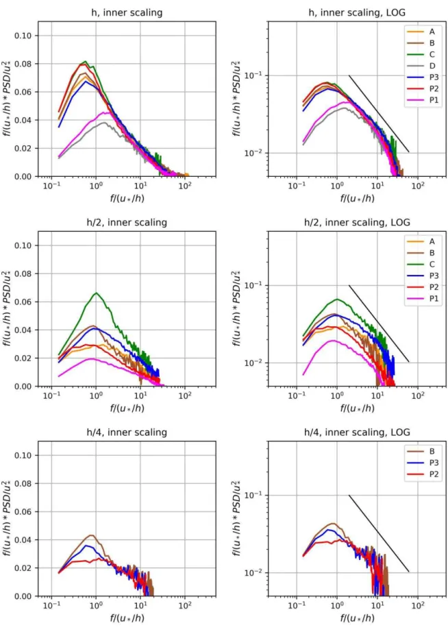
The spatial evolution of the power spectra of the streamwise velocity component at the different measurements points within wall-parallel planes inside the canopy is analyzed using Fig. 8 at z=h (top), z=h/2 (middle), and z=h/4 (bottom) with a linear-log representation (left) and a log-log representation (right). On the logarithmic representation, a black line with æt u slope is shown (equivalent to the æw u in the non-premultiplied form), to allow for comparison with the logarithmic region classically found in the inertial range of turbulent flows.
At the canopy interface (œLŠ), the energy is found to be spatially homogeneous, except in the downstream region of a cube (P1 and D), where the energy level is lower and shifted towards higher frequencies, which is probably the signature of the shear layer from the trailing edge of the cube. All spectra show a good collapse in the inertial subrange and display a logarithmic region with a slope close to æt u. At mid-height of the canopy (œLŠ t), there is more energy in a streamwise alley in between two cubes (C, P3, B), with the highest level at point C. An intermediate level is obtained in the upstream region (A, P2) and a low level is found again in the downstream region (P1) of a cube due to the low dynamic of the flow in the recirculation region. The spectra only tangentially approach the æt u region, and due to the variance of the spectra in the high-frequency region, a clear inertial region at the canopy mid-height cannot be evidenced. In any case, this region would be of fairly limited extent. Close to the wall (œ ŠLs v), we only have data at points P2, P3, and B. The maximum of energy is obtained at point B probably induced by high fluctuations due to the separation occurring on the side of the cube, as also observed at œ ŠLs t for point C (in close vicinity of B).
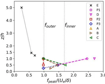
In Fig. 10 we report the frequency of the main energetic peak extracted for each measured point, while in Fig. 9, we report the average position of this peak in each wall-parallel planes. Overall, the average frequency of the main peak of energy is a decreasing function of wall-normal distance, possibly linked to a growing influence of the cubes on the dynamics of the flow. At point E in the inertial layer, the peak frequency is the lowest and reads fpeak = 0.25Ue ¼Å ; using a Taylor hypothesis, this yields a characteristic size of the large-scale motions of 3.3Å in the inertial layer.
Fig. 8 : Pre-multiplied power spectral density of the streamwise velocity component from LDA data, at all measurement points and at all heights, in linear-logarithmic scale (left column) and in logarithmic-logarithmic scale (right column)
When going down towards the wall, the peak frequency increases, with a change of slope at point E in the roughness sub-layer (z/h = 1.5), which can be interpreted as a footprint of the cube on the dynamics of the flow. Overall the average peak frequency shows a linear evolution in the region z/h Ð [0.5 ÷ 1.45]. The peak frequency is homogeneous at the canopy interface (z = h), with a peak frequency being located precisely at the characteristic frequency of outer-scaled motions fpeak = fouter = Ue ¼Å except for the downstream region of the cube (P1 and D) who have a peak frequency being more than twice as high as the other points due to their position within the shear layer developing from the top edge of the cube.
Deeper inside the canopy (z = h/2, h/4), there is more spatial heterogeneity. The peak frequency is the highest at the canopy mid-height, with the highest frequency obtained at points P3, C and B with fpeak § finner = uÛ/h, and then decreases towards a lower frequency at z/h = 1/4.
If the assumption is made that the shift towards higher frequencies is linked to the influence of the cube on the flow dynamics, then the downstream region of the cube (P1 and D) are the most impacted by the cube dynamics and the least impacted by the outer flow; on the contrary, the upstream region of the cube (P2) is the most impacted by the outer flow. In addition, it is likely that points having a peak frequency located between finner and fouter feel both dynamics of inner- and outer-flow, in connection with the complex scale-interactions in these regions.
Fig. 10 : Evolution of the peak of maximum energy of the pre-multi-plied power spectral density of the streamwise velocity component
Fig. 9 : Average position of the peak of maximum energy of the pre-multiplied power spectral density of the streamwise velocity component
4. Conclusion
The flow inside an idealized urban canopy consisting of a staggered array of cubes with a 25% density, immersed into an atmospheric boundary layer, has been investigated by means of Laser Doppler Anemometry. The flow conditions are relevant for real urban-like environments. Time-resolved measurements are realized at three heights in the canopy (œLŠ vá Š tá Š) and at different positions in wall-parallel planes. Great care is taken in estimating the temporal power spectra density, and a slight improvement of the refined Sample and Hold Algorithm (Nobach et al. 1998) is proposed to reduce the impact of measurement noise.
The analysis of the wall-normal evolution of the PSD of the streamwise velocity component shed some new light into the dynamics of urban canopy flows. The following noticeable facts are summarized below:
x in the inertial layer, the size of the large-scale motions given by the frequency of the main peak of energy is of the order of 3.3Å, as classically observed in turbulent wall-bounded flows;
x at the canopy interface and above a logarithmic region of slope close to -5/3 is evidenced; this is not the case deeper inside the canopy.
x the influence of the canopy is felt from the wall up the roughness sub-layer through a shift of energy towards higher frequencies with decreasing wall-normal distance;
x within the canopy, the inner and outer characteristic frequencies are felt by the flow, indicating the influence of both the outer and inner flow;
x a specific behavior of the flow is evidenced in the downstream region of the cube. A stronger energy cascade is visible through a lower level of energy and a characteristic frequency two-times higher than other points at the canopy interface. This indicates a stronger influence of the cube in this flow region.
Bibliography
Adrian RJ, Yao CS (1986) Power spectra of fluid velocities measured by laser Doppler velocimetry. Exp Fluids 5:17.28
Benedict LH, Nobach H, Tropea C (2000) Estimation of turbulent velocity spectra from laser Doppler data. Meas Sci Technol 11:1089
Blackman K, Perret L (2016) Non-linear interactions in a boundary layer developing over an array of cubes using stochastic estimation. Phys Fluids 28:095108. doi: 10.1063/1.4962938
Castro IP, Cheng H, Reynolds R (2006) Turbulence Over Urban-type Roughness: Deductions from Wind-tunnel Measurements. Bound-Layer Meteorol 118:109.131. doi: 10.1007/s10546-005-5747-7
Coceal O, Thomas TG, Castro IP, Belcher SE (2006) Mean Flow and Turbulence Statistics Over Groups of Urban-like Cubical Obstacles. Bound-Layer Meteorol 121:491.519. doi: 10.1007/s10546-006-9076-2
Grimmond CSB, Oke TR (1999) Aerodynamics properties of urban area derived from analysis of surface form. J Appl Meteorol
Herpin S, Perret L, Mathis R, et al (2018) Investigation of the flow inside an urban canopy immersed into an atmospheric boundary layer using laser Doppler anemometry. Exp Fluids 59:. doi: 10.1007/s00348-018-2532-1
Mayo Jr WT, Shay MT, Riter S (1974) The development of new digital data processing techniques for turbulence measurements with a laser velocimeter. Texas A&M University College Station, Texas
Nobach H (2016) A time-quantization based estimator for autocorrelation and spectral density estimation from laser Doppler anemometry data including local normalization
Nobach H, Müller E, Tropea C (1998) Efficient estimation of power spectral density from laser Doppler anemometer data. Exp Fluids 24:499.509. doi: 10.1007/s003480050199
Oke TR (1988) Street Design and Urban Canopy Layer Climate. Energy Build 103.113. doi: https://doi.org/10.1016/0378-7788(88)90026-6
Perret L, Basley J, Mathis R, Piquet T (2018) Atmospheric boundary layers over urban-like terrains: influence of the plan density on the roughness sublayer dynamics. Bound-Layer Meteorol in press:
Reynolds RT, Castro IP (2008) Measurements in an urban-type boundary layer. Exp Fluids 45:141. 156. doi: 10.1007/s00348-008-0470-z
Rivet C (2014) Etude en soufflerie atmosphérique des interactions entre canopée urbaine et basse atmosphère par PIV stéréoscopique. Ecole Centrale de Nantes
Van Maanen HRE, Nobach H, Benedict L van (1999) Improved estimator for the slotted autocorrelation function of randomly sampled LDA data. Meas Sci Technol 10:L4
Velte CM, George WK, Buchhave P (2014) Estimation of burst-mode LDA power spectra. Exp Fluids 55:. doi: 10.1007/s00348-014-1674-z
