Cross-population validation of statistical distance as a measure of physiological dysregulation
during aging
Alan A. Cohen, Emmanuel Milot, Qing Li, Véronique Legault, Linda P. Fried, and Luigi Ferrucci
Highlights
We validated statistical distance-aging associations in multiple human populations In all populations, statistical distance increases with age and predicts mortality This finding is not very sensitive to which biomarkers are used
Individual biomarkers alone behave differently across populations
1 2 3 4 5 6 7 8 9 10 11 12 13 14 15 16 17 18 19 20 21 22 23 24 25 26 27 28 29 30 31 32 33 34 35 36 37 38 39 40 41 42 43 44 45 46 47 48 49 50 51 52 53 54 55 56 57 58 59 60
Cross-population validation of statistical distance as a measure of physiological dysregulation
1
during aging
2
Alan A. Cohena*, Emmanuel Milota, Qing Lia, Véronique Legaulta, Linda P. Friedb, and Luigi Ferruccic 3
4
5
a
Groupe de recherche PRIMUS, Dept. of Family Medicine, University of Sherbrooke, CHUS-Fleurimont, 6
3001 12e Ave N, Sherbrooke, QC J1H 5N4, Canada 7
8
b
Mailman School of Public Health, Columbia University, 722 W. 168th Street, R1408, New York, NY 9
10032, USA 10
11
c
Clinical Research Branch, National Institute on Aging, National Institutes of Health, Longitudinal Studies 12
Section, Harbor Hospital, 3001 Hanover Street, Baltimore, Maryland 21225, USA 13
14
*Corresponding author: [email protected], (819) 346-1110 x12589, (819) 820-6419 (fax) 15
16
Word count: 2907; 1 Table; 3 Figures; 24 References 17
4 5 6 7 8 9 10 11 12 13 14 15 16 17 18 19 20 21 22 23 24 25 26 27 28 29 30 31 32 33 34 35 36 37 38 39 40 41 42 43 44 45 46 47 48 49 50 51 52 53 54 55 56 57 58 59 Abstract 18
Measuring physiological dysregulation during aging could be a key tool both to understand underlying 19
aging mechanisms and to predict clinical outcomes in patients. However, most existing indices are either 20
circular or hard to interpret biologically. Recently, we showed that statistical distance of 14 common 21
blood biomarkers (a measure of how strange an individual’s biomarker profile is) was associated with 22
age and mortality in the WHAS II data set, validating its use as a measure of physiological dysregulation. 23
Here, we extend the analyses to other data sets (WHAS I and InCHIANTI) to assess the stability of the 24
measure across populations. We found that the statistical criteria used to determine the original 14 25
biomarkers produced diverging results across populations; in other words, had we started with a 26
different data set, we would have chosen a different set of markers. Nonetheless, the same 14 markers 27
(or the subset of 12 available for InCHIANTI) produced highly similar predictions of age and mortality. 28
We include analyses of all combinatorial subsets of the markers and show that results do not depend 29
much on biomarker choice or data set, but that more markers produces a stronger signal. We conclude 30
that statistical distance as a measure of physiological dysregulation is stable across populations in 31
Europe and North America. 32
33
Keywords: Physiological dysregulation, aging, WHAS, InCHIANTI, biomarker, Mahalanobis distance 34
4 5 6 7 8 9 10 11 12 13 14 15 16 17 18 19 20 21 22 23 24 25 26 27 28 29 30 31 32 33 34 35 36 37 38 39 40 41 42 43 44 45 46 47 48 49 50 51 52 53 54 55 56 57 58 59 60 Introduction 36
Many researchers now believe that physiological dysregulation (or related processes such as 37
allostatic load and homeostenosis) are key players in the aging process, either as causal drivers of aging 38
or as accompanying processes that nonetheless produce important health consequences (Fried and 39
others 2005; Karlamangla and others 2002; McEwen and Wingfield 2003; Seplaki and others 2005; 40
Taffett 2003). These ideas propose that the complex regulatory networks that maintain homeostasis are 41
not infinitely robust, and that over time the network state might be perturbed in a way that prevents it 42
from returning fully to a baseline state(Cohen and others 2012). For instance, chronic stress results in 43
elevated baseline levels of cortisol, with numerous downstream consequences for health; the failure of 44
cortisol to return to baseline after a stress is an example of dysregulation (Miller and others 2007; 45
Sapolsky and others 2002). 46
A number of indices have been proposed to measure allostatic load, mostly for sociological or 47
epidemiological studies of population health (Crimmins and others 2003; Karlamangla and others 2002; 48
Seplaki and others 2005; Singer and others 2004; Yashin and others 2007). Most of these indices are 49
highly predictive of a variety of poor health outcomes (Goymann and Wingfield 2004; Gruenewald and 50
others 2009; Schnorpfeil and others 2003). However, the indices are generally composed of a number of 51
biomarkers or criteria already known to indicate poor health; it is thus unsurprising that individuals 52
doing poorly on multiple such measures have poor health outcomes. Accordingly the measures may be 53
useful as a summary of health state, but they do not validate the underlying hypothesis that 54
dysregulation is an important part of aging (Singer and others 2004). 55
Recently, we proposed a novel way to measure physiological dysregulation based on clinical 56
biomarkers (Cohen and others 2013). Under the hypothesis that a well-functioning, homeostatic 57
physiology should be relatively similar across individuals, but that there are many ways in which 58
physiology might become dysregulated, we proposed statistical distance (specifically Mahalanobis 59
4 5 6 7 8 9 10 11 12 13 14 15 16 17 18 19 20 21 22 23 24 25 26 27 28 29 30 31 32 33 34 35 36 37 38 39 40 41 42 43 44 45 46 47 48 49 50 51 52 53 54 55 56 57 58 59
distance, DM (De Maesschalck and others 2000; Mahalanobis 1936)) as a measure of physiological
60
dysregulation. DM (applied to biomarkers) is a measure of how strange an individual’s profile is relative
61
to everyone else in the population, and greater distance should thus measure greater dysregulation. We 62
applied this measure to a set of 14 biomarkers chosen from the Women’s Health and Aging Study 63
(WHAS) II data set based on their increase in deviance from the mean with age (but not necessarily 64
changes in the mean with age), and showed that DM increased with age within individuals and predicted
65
mortality controlling for age. Additionally, using the combinatorial subsets of the markers, we showed 66
that results were relatively insensitive to marker choice, but that predictive power increased with 67
inclusion of more markers in the calculation of DM. It thus appeared that DM is a measure of
68
physiological dysregulation. 69
However, a number of further validation steps are necessary before DM can be used widely. We need
70
to establish sensitivity to marker choice – including a wider array of markers – and to the choice of the 71
reference population used to define a “normal” biomarker profile. Also, predictive power for relevant 72
health outcomes needs to be assessed. Here, we tackle the question of reproducibility across 73
populations/data sets, asking whether similar results for the same 14 markers can be obtained in other 74
data sets. We use WHAS I (the complement study to WHAS II, including a less health segment of the 75
population in Baltimore, Maryland, USA) and Invecchiare in Chianti (InCHIANTI), a population-based 76
cohort study conducted in Tuscany, Italy. 77 78 Methods 79 Data 80
The Women’s Health and Aging Study (WHAS) is a population-based prospective study of 81
community-dwelling women. Originally, WHAS was two separate studies, WHAS I including 1002 women 82
aged 65+ among the 1/3 most disabled in the population(Fried and others 1995), and WHAS II including 83
4 5 6 7 8 9 10 11 12 13 14 15 16 17 18 19 20 21 22 23 24 25 26 27 28 29 30 31 32 33 34 35 36 37 38 39 40 41 42 43 44 45 46 47 48 49 50 51 52 53 54 55 56 57 58 59 60
436 women aged 70-79 among the 2/3 least disabled (Fried and others 2000). The participants were 84
drawn from eastern Baltimore City and Baltimore County, Maryland. Baseline assessment occurred from 85
November 1992 to February 1995 in WHAS I and from August 1994 to February 1996 in WHAS II. Eligible 86
non-participants were less educated, had lower incomes, and had lower self-rated health compared to 87
WHAS participants. Follow-ups were conducted roughly 1.5, 3, 6, 7.5, and 9 years later. Each 88
examination consisted of a comprehensive medical history, medication inventory, physical and 89
neurological examination, neuropsychological battery, and blood draw (Fried and others 2000). Here, 90
we merge participants from WHAS I and WHAS II into a single data set, WHAS, for comparison with 91
InCHIANTI. 92
Invecchiare in Chianti (InCHIANTI) is a prospective population-based study of 1156 adults aged 65-93
102 and 299 aged 20-64 randomly selected from two towns in Tuscany, Italy using multistage stratified 94
sampling in 1998 (Ferrucci and others 2000). Follow-up blood and urine samples were taken in 2001-03, 95
2005-06, and 2007-08. Because InCHIANTI contains both men and younger individuals, we replicate 96
InCHIANTI analyses on the subset of women aged 70+ in order to have a population comparable to 97
WHAS II in our previous study. 98
99
Biomarker choice
100
In our previous study (Cohen and others 2013), 14 biomarkers were chosen from among 63 101
candidate markers based on a positive correlation of their deviances with age (the deviance is the 102
absolute value of the marker level minus the population mean). Here, we use the same markers: red 103
blood cell count, hemoglobin, hematocrit, sodium, chloride, potassium, calcium, cholesterol, albumin, 104
creatinine, BUN:creatinine ration, basophil count, osteocalcin, and direct bilirubin, although the last two 105
were not measured in InCHIANTI and are thus excluded from those analyses. We also compared 106
whether we would have chosen the same set of markers had we applied the same criteria to the data 107
4 5 6 7 8 9 10 11 12 13 14 15 16 17 18 19 20 21 22 23 24 25 26 27 28 29 30 31 32 33 34 35 36 37 38 39 40 41 42 43 44 45 46 47 48 49 50 51 52 53 54 55 56 57 58 59
sets used here, calculating the correlation of each biomarker with age, and of its deviance with age, in 108 each population. 109 110 Statistical analyses 111
All statistical analyses were conducted in R v3.0.1 and code is available upon request. All variables 112
were log- or square-root-transformed as necessary to approach normality, and then standardized by 113
subtracting their mean and dividing by their standard deviation. DM was calculated using the following
114
formula: 115
(1)
116
where x is a multivariate observation (a vector of simultaneously observed values for the variables in 117
question, such as all the biomarker values for a given patient at a given time point), is the equivalent-118
length vector of population means for each variable, and S is the population variance-covariance matrix 119
for the variables. The parameters and S were estimated for each data set) from the first visit of each 120
individual, both to assure independence of observations and to use a slightly younger, healthier 121
reference population. Because DM is approximately log-normally distributed, it was log-transformed
122
before analysis. 123
Individual changes in DM with age were modeled using linear regression models for each individual to
124
estimate a slope for each individual; weighted t-tests were then used to assess whether the slope was 125
significantly different from zero, weighted by the number of observations per individual. The mean slope 126
per population was thus a measure of rate of change of DM with age. The relationship between DM and
127
subsequent mortality was modeled using Cox proportional hazards models (coxph function, 128
survival package) using a time-to-event framework and age as the time variable. 129
4 5 6 7 8 9 10 11 12 13 14 15 16 17 18 19 20 21 22 23 24 25 26 27 28 29 30 31 32 33 34 35 36 37 38 39 40 41 42 43 44 45 46 47 48 49 50 51 52 53 54 55 56 57 58 59 60
All analyses were repeated for each combinatorial subset of the variables (16,383 combinations for 130
the 14 variables in WHAS and 4095 combinations for the 12 variables in InCHIANTI), and meta-131
regression models were used to assess the impact of the number of variables and which variables were 132
included on model results. Results were also merged across data sets by biomarker combination to 133
assess correlations of results across data sets for the same biomarker combinations. All analyses were 134
repeated for WHAS I, WHAS II, InCHIANTI, WHAS I and II combined, and the subset of InCHIANTI that is 135
women aged 70+. The latter was chosen to have a population comparable with the original WHAS II 136 study. 137 138 Results 139
Correlations of deviances with age were markedly heterogeneous across data sets (Fig. 1). There was 140
very little correspondence across data sets as to which variables would have been retained for use in DM
141
(i.e., those with significant positive deviance correlations with age, shaded blue in Fig. 1), with only one 142
of the original 12 shared across WHAS I, WHAS II, and InCHIANTI. Restricting InCHIANTI to women aged 143
70+ so that its composition resembled WHAS II did not improve the correspondence. Raw correlations 144
with age were more often significant than deviance correlations, and showed somewhat greater (but 145
4 5 6 7 8 9 10 11 12 13 14 15 16 17 18 19 20 21 22 23 24 25 26 27 28 29 30 31 32 33 34 35 36 37 38 39 40 41 42 43 44 45 46 47 48 49 50 51 52 53 54 55 56 57 58 59
not much) consistency across data sets. 146
147
Figure 1: Correlations of raw variables and their deviances with age. Variables are sorted from lowest to highest deviance 148
correlation coefficient in WHAS II (third column). Colored boxes indicate significant correlations (blue=positive, red=negative) 149
with darker shading indicating lower p-values. Note that of the 12 original variables retained for WHAS II (those shaded blue at 150
the bottom), only one would have been retained for WHAS I and four for InCHIANTI. On the other hand, eight additional 151
variables not retained for WHAS II would have been retained for WHAS I, and 18 for InCHIANTI. 152
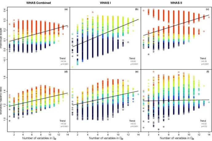
For all data sets, most combinations of biomarkers produced DMs that increased with age (positive
153
individual slope) and that positively predicted mortality (Figs 2-3). For change with age, 82% of analyses 154
were significant at α=0.05 in WHAS and 99% in InCHIANTI; for mortality, 73% were significant in WHAS 155
and 83% in InCHIANTI. Given the consistently positive relationships with mortality (99.9% of models in 156 Vitamin D 25OH SHBG Ferritin a-Tocoph Alk phosph SGPT Folate IGF-1 TIBC WBCs a-Carot EPO MAP Thy roxine GGT MCV Vitamin B12 B-Cry ptox Neutrophils RDW MCHC CRP EOS DHEAS Vitamin B6 PTHB intact Ly copene TSH A-G ratio Selenium PTHB mid-region HDL Ly mphocy tes Glucose Iron B-Carot MCH Zeaxanthin Testosterone Vitamin A SGOT Total protein Trigly cerides MPV Platelets Monocy tes IL-6 LDH Estradiol Magnesium Uric acid Chloride Albumin Hematocrit Free testost Potassium Hemoglobin Calcium RBCs BASO Cholest Sodium Creatinine BUN-Creat ratio
Deviance correlations Raw correlations
WHAS InCHIANTI WHAS InCHIANTI
4 5 6 7 8 9 10 11 12 13 14 15 16 17 18 19 20 21 22 23 24 25 26 27 28 29 30 31 32 33 34 35 36 37 38 39 40 41 42 43 44 45 46 47 48 49 50 51 52 53 54 55 56 57 58 59 60
both WHAS and InCHIANTI) and the generally large effect sizes (median hazard ratio per unit DM of 1.27
157
for WHAS and 1.20 for InCHIANTI), the lower levels of significant results for mortality are likely due to 158
less statistical power as a result of the relatively limited number of deaths in the data sets (up to 122 in 159
WHAS and 193 in InCHIANTI, depending on the biomarker combination and missingness). 160
161
Figure 2: Changes in predictive power of DM in WHAS with increasing numbers of variables used in its calculation. Each circle 162
represents an analysis based on one of the 16383 combinatorial subsets of the 14 variables in WHAS. Color indicates p-value: 163
black: p ≥ 0.1; blue: 0.05 ≤ p < 0.1; cyan: 0.01 ≤ p < 0.05; yellow-green: 0.001 ≤ p < 0.01; orange: 0.0001 ≤ p < 0.001; red: p < 164
0.0001. The line represents a linear regression of number of variables on relevant effect size. Effect size trend shows the results 165
of a Pearson correlation analysis of variable number with relevant effect size. (a)-(c): average individual slope of DM with age 166
(units of increase in DM per year). (d)-(f): hazard ratio of mortality per unit DM, controlling for age. (a), (d): The full WHAS data 167
set. (b), (e): WHAS I. (c), (f): WHAS II. 168
In all cases there was a significant tendency to have stronger predictions with more variables 169
included in the calculation of DM (Figs 2-3). In general this effect was quite large, with age slopes
170
generally about twice as large when DM was calculated with the maximum 14 or 12 variables, compared
4 5 6 7 8 9 10 11 12 13 14 15 16 17 18 19 20 21 22 23 24 25 26 27 28 29 30 31 32 33 34 35 36 37 38 39 40 41 42 43 44 45 46 47 48 49 50 51 52 53 54 55 56 57 58 59
to just one variable. Hazard ratios were often 50% larger with maximum number of variables, except for 172
in WHAS II, where the effect was negligible (Fig. 2f). 173
174
Figure 3: Changes in predictive power of DM in InCHIANTI with increasing numbers of variables used in its calculation. Each 175
circle represents an analysis based on one of the 4095 combinatorial subsets of the 12 variables in InCHIANTI. Color indicates p-176
value: black: p ≥ 0.1; blue: 0.05 ≤ p < 0.1; cyan: 0.01 ≤ p < 0.05; yellow-green: 0.001 ≤ p < 0.01; orange: 0.0001 ≤ p < 0.001; red: 177
p < 0.0001. The line represents a linear regression of number of variables on relevant effect size. Effect size trend shows the
178
results of a Pearson correlation analysis of variable number with relevant effect size. (a) and (b): average individual slope of DM 179
with age (units of increase in DM per year). (c) and (c): hazard ratio of mortality per unit DM, controlling for age. (a) and (c): The 180
full InCHIANTI data set. (b) and (d): The subset of women aged 70+ (for comparison with the original WHAS II data set). 181
We also tested whether results were correlated between WHAS and InCHIANTI for the same variable 182
combination. For slope with age, the correlation was quite strong (r=0.74, p<0.0001), but this was 183
mostly due to the inclusion or exclusion of one variable, basophil count. Stratifying by basophil count, 184
4 5 6 7 8 9 10 11 12 13 14 15 16 17 18 19 20 21 22 23 24 25 26 27 28 29 30 31 32 33 34 35 36 37 38 39 40 41 42 43 44 45 46 47 48 49 50 51 52 53 54 55 56 57 58 59 60
the correlation was much weaker (r=0.22 with basophils and r=0.26 without, p<0.0001 for both). This 185
was similar to the correlation for hazard ratios (r=0.28, p<0.0001). These correlations are surprisingly 186
weak: the performance of models in one data set explains only 5-8% of the variance the performance in 187
the other (calculated as the squares of the pairwise correlation coefficients). 188
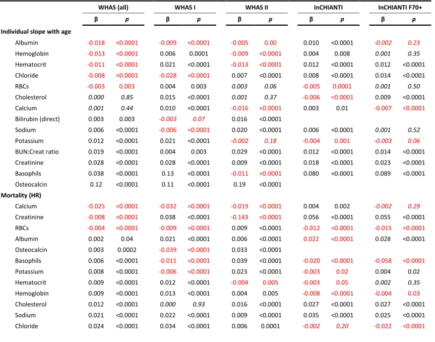
Results were also quite heterogeneous for the effects of including or excluding each biomarker in the 189
calculation of DM (Table 1). Almost all the effects (89%) were significant at α=0.05, but in all but six of
190
the 28 cases (14 variables 2 outcomes) these significant effects went in opposing directions depending 191
on the data set or subset. The six cases were as follows: including creatinine, BUN:creatinine ratio, and 192
osteocalcin significantly increased the slope with age, and including bilirubin, sodium, and cholesterol 193
significantly increased hazard ratios. The effect for osteocalcin was quite large, explaining the nearly 194
separate point clouds in Fig 2c. Despite one result to the contrary for WHAS II, including basophil count 195
also appears to have a generally strong, positive effect on slope, explaining the separate point clouds in 196
Fig. 3a-b for InCHIANTI. Note, however, that the variables that improve model performance for change 197
in DM with age are not the same as those that improve mortality prediction.
4 5 6 7 8 9 10 11 12 13 14 15 16 17 18 19 20 21 22 23 24 25 26 27 28 29 30 31 32 33 34 35 36 37 38 39 40 41 42 43
Table 1: Results of metagregression analyses to assess the impact of including or excluding each variable in the calculation of DM 199
WHAS (all) WHAS I WHAS II InCHIANTI InCHIANTI F70+
β p β p β p β p β p
Individual slope with age
Albumin -0.018 <0.0001 -0.009 <0.0001 -0.005 0.00 0.010 <0.0001 -0.002 0.23 Hemoglobin -0.013 <0.0001 0.006 0.0001 -0.009 <0.0001 0.004 0.008 0.001 0.35 Hematocrit -0.011 <0.0001 0.021 <0.0001 -0.013 <0.0001 0.012 <0.0001 0.012 <0.0001 Chloride -0.008 <0.0001 -0.028 <0.0001 0.007 <0.0001 0.008 <0.0001 0.014 <0.0001 RBCs -0.003 0.003 0.004 0.003 0.003 0.06 -0.005 0.0001 0.001 0.50 Cholesterol 0.000 0.85 0.015 <0.0001 0.001 0.37 -0.006 <0.0001 0.009 <0.0001 Calcium 0.001 0.44 0.010 <0.0001 -0.016 <0.0001 0.003 0.01 -0.007 <0.0001 Bilirubin (direct) 0.003 0.003 -0.003 0.07 0.016 <0.0001 Sodium 0.006 <0.0001 -0.006 <0.0001 0.020 <0.0001 0.006 <0.0001 0.001 0.52 Potassium 0.012 <0.0001 0.021 <0.0001 -0.002 0.18 -0.004 0.001 -0.003 0.06 BUN:Creat ratio 0.019 <0.0001 0.004 0.003 0.029 <0.0001 0.012 <0.0001 0.014 <0.0001 Creatinine 0.028 <0.0001 0.028 <0.0001 0.009 <0.0001 0.018 <0.0001 0.023 <0.0001 Basophils 0.038 <0.0001 0.13 <0.0001 -0.011 <0.0001 0.080 <0.0001 0.089 <0.0001 Osteocalcin 0.12 <0.0001 0.11 <0.0001 0.19 <0.0001 Mortality (HR) Calcium -0.025 <0.0001 -0.032 <0.0001 -0.019 <0.0001 0.004 0.002 -0.002 0.29 Creatinine -0.008 <0.0001 0.038 <0.0001 -0.143 <0.0001 0.056 <0.0001 0.055 <0.0001 RBCs -0.004 <0.0001 -0.009 <0.0001 0.009 <0.0001 -0.012 <0.0001 -0.015 <0.0001 Albumin 0.002 0.04 0.021 <0.0001 0.006 <0.0001 0.022 <0.0001 0.028 <0.0001 Osteocalcin 0.003 0.0002 -0.039 <0.0001 0.033 <0.0001 Basophils 0.006 <0.0001 -0.011 <0.0001 0.039 <0.0001 -0.020 <0.0001 -0.058 <0.0001 Potassium 0.008 <0.0001 -0.006 <0.0001 0.023 <0.0001 -0.003 0.02 0.004 0.02 Hematocrit 0.009 <0.0001 0.012 <0.0001 -0.004 0.005 -0.003 0.05 0.002 0.35 Hemoglobin 0.009 <0.0001 0.013 <0.0001 0.004 0.005 -0.008 <0.0001 -0.004 0.03 Cholesterol 0.012 <0.0001 0.000 0.93 0.016 <0.0001 0.027 <0.0001 0.027 <0.0001 Sodium 0.021 <0.0001 0.022 <0.0001 0.009 <0.0001 0.035 <0.0001 0.025 <0.0001 Chloride 0.024 <0.0001 0.034 <0.0001 0.006 0.0001 -0.002 0.20 -0.022 <0.0001
4 5 6 7 8 9 10 11 12 13 14 15 16 17 18 19 20 21 22 23 24 25 26 27 28 29 30 31 32 33 34 35 36 37 38 39 40 41 42 43 44 BUN:Creat ratio 0.042 <0.0001 0.057 <0.0001 -0.011 <0.0001 0.014 <0.0001 0.023 <0.0001 Bilirubin (direct) 0.062 <0.0001 0.068 <0.0001 0.049 <0.0001 Betas indicate change in effect size with the inclusion of the biomarker. Biomarkers are ordered by their beta-coefficients for the full WHAS data set, separately for individual slope with age and mortality. Negative coefficients are marked in red; coefficients not significant at alpha=0.05 are in italics.
4 5 6 7 8 9 10 11 12 13 14 15 16 17 18 19 20 21 22 23 24 25 26 27 28 29 30 31 32 33 34 35 36 37 38 39 40 41 42 43 44 45 46 47 48 49 50 51 52 53 54 55 56 57 58 59 Discussion 200
The results presented here confirm and expand on our previous study showing that statistical 201
distance is a promising measure for physiological dysregulation during aging (Cohen and others 2013). 202
By using additional data sets (WHAS I and InCHIANTI), we are able to provide independent confirmation 203
of those results, results which are nearly identical in terms of the big picture (Figs 2-3), but which are 204
also surprisingly different in the details. In all data sets, DM significantly increases with age within
205
individuals, and significantly predicts mortality. Likewise, in all cases predictions improve as more 206
variables are included in the calculation of DM. These three findings confirm key predictions about how
207
DM should behave if it is truly a measure of physiological dysregulation (Cohen and others 2013).
208
One of the key challenges in developing a measure of physiological dysregulation is to avoid 209
circularity (Singer and others 2004). It is unsurprising that by combining multiple measures of poor 210
health one arrives at a measure that predicts poor health or age. Statistical distance, as measured by DM,
211
circumvents this problem by asking not if each patient is badly off on each marker, but by asking 212
whether the overall profile of markers is far from average, regardless of how we define a healthy state 213
for each. Additionally, we specifically did not restrict marker choice to those known to change with age 214
or with health status; electrolyte levels, for example, are generally quite stable outside of specific 215
pathologies. However, in our original study, we did impose the criterion that the deviance of markers 216
from their mean be positively correlated with age (i.e., more aberrant values at older ages) in order to 217
try to choose markers that would provide a stronger signal (Cohen and others 2013). Here, we showed 218
that even this criterion is largely irrelevant – the correlations of individual markers with age are often 219
quite heterogeneous across data sets and even subsets, and the correlations of the deviances with age 220
are even more so. We would have chosen a completely different suite of markers had our original data 221
set been a different one; nonetheless, using the markers chosen based on WHAS II, we get nearly 222
identical results in all the data sets. 223
4 5 6 7 8 9 10 11 12 13 14 15 16 17 18 19 20 21 22 23 24 25 26 27 28 29 30 31 32 33 34 35 36 37 38 39 40 41 42 43 44 45 46 47 48 49 50 51 52 53 54 55 56 57 58 59 60
Likewise, we expected that a given combination of markers would provide a similar signal in different 224
data sets, but the correlations were surprisingly weak. In each data set, the inclusion or exclusion of 225
each marker was almost always significantly associated with model performance, but the directions of 226
these associations varied across data sets, and few markers showed consistent effects across data sets. 227
No markers showed consistent effects both (a) predicting both age and mortality, and (b) across data 228
sets. In other words, if we find that including a given marker in the calculation of DM improves the
229
performance of DM in one data set, we cannot necessarily make any inferences from this toward other
230
data sets, at least among the markers used here. 231
How can we explain these relatively inconsistent results model-by-model, despite consistent results 232
at a higher level? We believe that the discrepancies across data sets are, counterintuitively, a 233
confirmation of the generality of DM as a measure of dysregulation. If the performance of DM depended
234
too heavily on the choice of marker, it would suggest that DM is not a measure of generalized
235
dysregulatory state, but rather of what is happening with several key markers. Heterogeneity of results 236
suggests that the effects of each marker of DM performance depend on small differences across data
237
sets in terms of population composition, diet, lifestyle, underlying physiology, and so forth; nonetheless, 238
by combining a sufficient number of markers (and without much regard for which) we are able to 239
circumvent these details and arrive at a fairly robust, generalized signal of dysregulatory state. Given 240
what is known about the complexity of physiological regulation, this is in fact exactly the prediction we 241
would make if DM truly represents physiological dysregulation.
242
At a practical level, this study supports the utility of DM as a measure of dysregulation or generalized
243
health state, whether it be in studies of aging epidemiology, sociological or economic studies of 244
population health, or in clinic. Clinical frailty measures such as Fried’s frailty criteria (Fried and others 245
2001) and the Frailty Index (Rockwood and others 2005) provide useful insight into functional decline 246
during aging (Clegg and others 2013); DM promises to be a complementary measure of the underlying
4 5 6 7 8 9 10 11 12 13 14 15 16 17 18 19 20 21 22 23 24 25 26 27 28 29 30 31 32 33 34 35 36 37 38 39 40 41 42 43 44 45 46 47 48 49 50 51 52 53 54 55 56 57 58 59
physiology. While frailty measures are most powerful late in life, DM appears to pick up a signal much
248
younger, suggesting clinical applications in prevention and non-geriatric populations, as well as 249
coordinated use with frailty measures. 250
However, several further validation steps are necessary before implementing DM widely. First,
251
robustness/sensitivity to marker choice and number needs to be established across a wider array of 252
markers, and recommended optimal marker combinations should be established. Second, we need to 253
understand the sensitivity to reference population (the population used to establish the definition of a 254
“normal” or “average” profile). Given that most of the individuals used here were already elderly and 255
thus in poorer health, there may be a potential to achieve better performance using younger and/or 256
healthier populations to compute and S in equation (1). Third, predictive value of DM for specific
257
health outcomes such as frailty and cardiovascular disease needs to be assessed. Fourth, we will need to 258
analyze whether there is a single global dysregulatory process, or if dysregulation can be usefully 259
subdivided by physiological or biological system, and, in the latter case, if these dysregulations are 260
correlated. 261
While such validation is essential before systematic implementation, current results are strong 262
enough to suggest that DM could be useful immediately in smaller-scale studies. For example, we were
263
recently able to successfully predict two measures of health state in a population of wild birds based on 264
DM calculated from 11 biomarkers available in an existing data set (Milot and others 2013). Additionally,
265
at a theoretical level, this study confirms the interpretation of DM as a measure of physiological
266
dysregulation, as well as a role for physiological dysregulation in the aging process. It suggests strongly 267
that too much emphasis on any single molecule may be misleading (as seen from our differing results for 268
each molecule across data sets), and that measures of system-level properties of regulatory state will be 269
necessary to better understand the aging process. 270
4 5 6 7 8 9 10 11 12 13 14 15 16 17 18 19 20 21 22 23 24 25 26 27 28 29 30 31 32 33 34 35 36 37 38 39 40 41 42 43 44 45 46 47 48 49 50 51 52 53 54 55 56 57 58 59 60 Acknowledgements 272
AAC is a member of the FRQ-S-supported Centre de recherche sur le vieillissement and Centre de 273
recherche Étienne Le-Bel, and is a funded Research Scholar of the FRQ-S. This research was supported by
274
CIHR grant #s 110789, 120305, 119485 and by NSERC Discovery Grant # 402079-2011. 275
276
References 277
Clegg, A.; Young, J.; Iliffe, S.; Rikkert, M.O.; Rockwood, K. Frailty in elderly people. The Lancet. 381:752-278
762; 2013 279
Cohen, A.A.; Martin, L.B.; Wingfield, J.C.; McWilliams, S.R.; Dunne, J.A. Physiological regulatory 280
networks: ecological roles and evolutionary constraints. Trends in Ecology & Evolution. 27:428-281
435; 2012 282
Cohen, A.A.; Milot, E.; Yong, J.; Seplaki, C.L.; Fülöp, T.; Bandeen-Roche, K.; Fried, L.P. A novel statistical 283
approach shows evidence for multi-system physiological dysregulation during aging. 284
Mechanisms of Ageing and Development. 134:110-117; 2013 285
Crimmins, E.M.; Johnston, M.; Hayward, M.; Seeman, T. Age differences in allostatic load: an index of 286
physiological dysregulation. Experimental Gerontology. 38:731-734; 2003 287
De Maesschalck, R.; Jouan-Rimbaud, D.; Massart, D.L. The Mahalanobis distance. Chemometrics and 288
Intelligent Laboratory Systems. 50:1-18; 2000 289
Ferrucci, L.; Bandinelli, S.; Benvenuti, E.; Di Iorio, A.; Macchi, C.; Harris, T.B.; Guralnik, J.M. Subsystems 290
contributing to the decline in ability to walk: bridging the gap between epidemiology and 291
geriatric practice in the InCHIANTI study. Journal of the American Geriatrics Society. 48:1618-292
1625; 2000 293
Fried, L.P.; Bandeen-Roche, K.; Chaves, P.H.; Johnson, B.A. Preclinical mobility disability predicts incident 294
mobility disability in older women. Journal of gerontology Series A, Biological sciences and 295
medical sciences. 55:M43-M52; 2000 296
Fried, L.P.; Hadley, E.C.; Walston, J.D.; Newman, A.B.; Guralnik, J.M.; Studenski, S.; Harris, T.B.; Ershler, 297
W.B.; Ferrucci, L. From Bedside to Bench: Research Agenda for Frailty. Sci Aging Knowl Environ. 298
2005:pe24-; 2005 299
Fried, L.P.; Kasper, K.D.; Guralnik, J.M.; Simonsick, E.M. The Women's Health and Aging Study: an 300
introduction. in: Guralnik J.M., Fried L.P., Simonsick E.M., Kasper K.D., Lafferty M.E., eds. The 301
Women's Health and Aging Study: health and social characteristics of old women with disability. 302
Bethesda, MD: National Institute on Aging; 1995 303
Fried, L.P.; Tangen, C.M.; Walston, J.; Newman, A.B.; Hirsch, C.; Gottdiener, J.; Seeman, T.E.; Tracy, R.; 304
Kop, W.J.; Burke, G.; McBurnie, M.A. Frailty in Older Adults: Evidence for a Phenotype Journal of 305
gerontology Series A, Biological sciences and medical sciences. 56:M146-M157; 2001 306
Goymann, W.; Wingfield, J.C. Allostatic load, social status and stress hormones: the costs of social status 307
matter. Animal Behaviour. 67:591-602; 2004 308
Gruenewald, T.L.; Seeman, T.E.; Karlamangla, A.S.; Sarkisian, C.A. Allostatic Load and Frailty in Older 309
Adults. Journal of the American Geriatrics Society. 57:1525-1531; 2009 310
Karlamangla, A.S.; Singer, B.H.; McEwen, B.S.; Rowe, J.W.; Seeman, T.E. Allostatic load as a predictor of 311
functional decline: MacArthur studies of successful aging. Journal of Clinical Epidemiology. 312
55:696-710; 2002 313
4 5 6 7 8 9 10 11 12 13 14 15 16 17 18 19 20 21 22 23 24 25 26 27 28 29 30 31 32 33 34 35 36 37 38 39 40 41 42 43 44 45 46 47 48 49 50 51 52 53 54 55 56 57 58 59
Mahalanobis, P.C. Mahalanobis distance. Proceedings National Institute of Science of India. 49:234-256; 314
1936 315
McEwen, B.S.; Wingfield, J.C. The concept of allostasis in biology and biomedicine. Hormones and 316
Behavior. 43:2-15; 2003 317
Miller, G.E.; Chen, E.; Zhou, E.S. If it goes up, must it come down? Chronic stress and the hypothalamic-318
pituitary-adrenocortical axis in humans. Psychological Bulletin. 133:25-45; 2007 319
Milot, E.; Cohen, A.A.; Vézina, F.; Buehler, D.M.; Matson, K.D.; Piersma, T. A novel integrative method for 320
measuring body condition in ecological studies based on physiological dysregulation. Methods in 321
Ecology and Evolution:n/a-n/a; 2013 322
Rockwood, K.; Song, X.; MacKnight, C.; Bergman, H.; Hogan, D.B.; McDowell, I.; Mitnitski, A. A global 323
clinical measure of fitness and frailty in elderly people. CMAJ. 173:489-495; 2005 324
Sapolsky, R.M.; Krey, L.C.; McEwen, B.S. The Neuroendocrinology of Stress and Aging: The Glucocorticoid 325
Cascade Hypothesis. Sci Aging Knowl Environ. 2002:cp21-; 2002 326
Schnorpfeil, P.; Noll, A.; Schulze, R.; Ehlert, U.; Frey, K.; Fischer, J.E. Allostatic load and work conditions. 327
Social Science & Medicine. 57:647-656; 2003 328
Seplaki, C.L.; Goldman, N.; Glei, D.; Weinstein, M. A comparative analysis of measurement approaches 329
for physiological dysregulation in an older population. Experimental Gerontology. 40:438-449; 330
2005 331
Singer, B.H.; Ryff, C.D.; Seeman, T. Operationalizing allostatic load. in: Schuli J., ed. Allostasis, 332
Homeostasis, and the Costs of Physiological Adaptation. Cambridge, UK: Cambridge University 333
Press; 2004 334
Taffett, G.E. Physiology of Aging. in: Cassel C.K., Leipzig R.M., Cohen H.J., Larson E.B., Meier D.E., Capello 335
C.F., eds. Geriatric Medicine: Springer New York; 2003 336
Yashin, A.I.; Arbeev, K.G.; Akushevich, I.; Kulminski, A.; Akushevich, L.; Ukraintseva, S.V. Stochastic model 337
for analysis of longitudinal data on aging and mortality. Mathematical Biosciences. 208:538-551; 338
2007 339
340 341