HAL Id: hal-02376817
https://hal.archives-ouvertes.fr/hal-02376817
Submitted on 22 Nov 2019
HAL is a multi-disciplinary open access
archive for the deposit and dissemination of
sci-entific research documents, whether they are
pub-lished or not. The documents may come from
teaching and research institutions in France or
abroad, or from public or private research centers.
L’archive ouverte pluridisciplinaire HAL, est
destinée au dépôt et à la diffusion de documents
scientifiques de niveau recherche, publiés ou non,
émanant des établissements d’enseignement et de
recherche français ou étrangers, des laboratoires
publics ou privés.
Temporal extensions of nonnegative matrix factorization
Cédric Févotte, Paris Smaragdis, Nasser Mohammadiha, Gautham Mysore
To cite this version:
Cédric Févotte, Paris Smaragdis, Nasser Mohammadiha, Gautham Mysore. Temporal extensions of
nonnegative matrix factorization. Audio Source Separation and Speech Enhancement, 2018.
�hal-02376817�
1
Temporal extensions of nonnegative matrix
factorization
Cédric Févotte, Paris Smaragdis, Nasser Mohammadiha and Gautham J. Mysore
Temporal continuity is one of the most important features of time series data. Our aim here is to present some of the basic as well as advanced ideas to make use of this information by modeling time dependencies in NMF. The dependencies between consecutive frames of the spectrogram can be imposed either on the basis matrix B or on the activations H (introduced in Chapter 8). The former case is known as the convolutive NMF, reviewed in Section 1.1. In this case, the repeating patterns within data are represented with multidimensional bases which are not vectors anymore, but functions that can span an arbitrary number of dimensions (e.g., time and fre-quency). The other case consists in imposing temporal structure on the activations H, in line with traditional dynamic models that have been studied extensively in sig-nal processing. Most models considered in the NMF literature can be cast as special cases of a unifying state-space models that will be discussed in Section 1.2. Special cases will be reviewed in subsequent sections. Continuous models are addressed in Sections 1.3 and 1.4, while Section 1.5 reviews models that involve a discrete latent state variable. Sections 1.6 and 1.7 provide quantitative and qualitative comparisons of the proposed methods, while Section 1.8 summarizes. This chapter is an extended version of the review paper (Smaragdis et al., 2014).
In this chapter, we will denote by bVthe nonnegative spectral data, with columns ˆ
v(n)and coefficients ˆvf n. In most cases, bVis either the magnitude spectrogram |X|
or the power spectrogram |X|2, i.e., ˆv
f n = |x(n, f)| or |x(n, f)|2. We will also
denote V = BH, with coefficients vf n. Note that traditionally the NMF literature
instead denotes the data by V and the approximate factorization by bV. However the chosen notation is here consistent with the convention used in this book, where variable with a hat denote statistics (observed quantities) and variables without a hat denote model parameters.
6
1.1
Convolutive NMF
Convolutive NMF (Smaragdis, 2007; O’Grady and Pearlmutter, 2008; Wang et al., 2009) is a technique that is used to model each sound source as a collection of time-frequency templates that each span multiple time frames and/or time-frequency bins (of-ten all frequency bins). As we will show shortly, these templates of(of-ten correspond to basic elements of sounds, such as phonemes of speech, notes of music, or other tem-porally coherent units of sound. By using this approach, we can capture a lot of the temporally important nuances that make up a given sound. However, since it directly captures a whole time-frequency patch, it can be quite inflexible and can not model sounds of varying lengths and pitches. For example, a template of a given vowel will have difficulty modeling the same vowel of a longer length or different pitch. On the other hand, sounds of a fixed length and pitch, such as a drum hit, can be modeled quite well using this technique. These models can be seen as a deterministic way to model temporal dependencies.
1.1.1
1-D Convolutive NMF
We will start by formulating the 1-dimensional (1-D) version of convolutive NMF and build up from there. Recall that traditional NMF performs the approximation:
b
V⇡ BH (1.1)
where B 2 RF⇥K
+ and H 2 RK+⇥Nare the K bases and activations respectively
(see Chapter 8). A significant shortcoming of this model is that the temporal struc-ture of the input signal is not represented in any way. The basis matrix B will contain a set of spectra that can be used to compose an input sound, but there is no represen-tation of their temporal relationships. In order to address this problem we consider an alternative decomposition that explicitly encodes sequences of spectra. We start using the following formulation:
v(n)(n,· · · , N0+ n) = B(n)H (1.2)
b
V⇡X
n
v(n) (1.3)
where v(n)(n,· · · , N0+n)represents an additive part of the n-th to N0+ncolumns
(time frames) of bV. The constant N0is chosen so that for the maximum value of n
we would have N = N0+ n, for reasons that should become clear momentarily.
There are a couple of observations to make about this model. First of all, we now have a different representation of the bases. Instead of a single basis matrix B, where each column is a basis, we have a set of basis matrices B(n), where the parenthesized
index relates to a time shift relating to its input. We note that each of these matrices is used to approximate a time-shifted version of the input and that all these matrices share the same activations patterns. By doing so we effectively force the bases of
B(n+1)to always get activated the same way as the bases of B(n)have been in the
previous time frame. In other words, we would always expect to see the kth basis of B(n)to be followed in the next time frame by the kth basis of B(n+1), etc. By doing
so we create a set of bases that have a deterministic temporal evolution which spans as many time steps as we have B(n)matrices.
To consider the effects of this new structure let us consider the toy input shown in Fig. 1.1. The toy input in this case is shown in the top right panel and consists of a “spectrogram” that contains two types of repeating patterns. One pattern consists of two parallel components which over time drop by one frequency bin for a dura-tion of two frames, and another consists of two components which similarly rise in frequency. Although we could decompose this input using a regular NMF model, the resulting representation would not be very illuminating (it would be a set of 6 unordered bases, not revealing temporal structure very clearly). Instead we analyze this using the model above. We will ask for three matrices B(n), n2 {1, 2, 3}, each
being made up by two bases B(n) 2 RF⇥2+ . This will allow us to learn two
time-frequency components which extend for three time frames each. Since this is exactly the structure in the input, we would expect to effectively learn the patterns therein. After estimating these parameters, we show the results in the remaining plots in the same figure. At the top left we see the three matrices B(n). Note that the nth matrix
will contain the nth time frame of all the bases. Below these plots we show the same information reordered so that each basis is grouped with its temporal components. In order to obtain the kth convolutive basis Bk, we use:
Bk =⇥B(1)(k), B(2)(k), B(3)(k),· · ·
⇤ (1.4)
i.e. in the case of figure 1.1 for the first basis we would concatenate the matrices B(1)(1), B(2)(1), B(3)(1). Doing so, we now clearly see that the two learned bases
have a temporal structure that reflects the input. The first one contains two rising components, and the second one contains two descending components. These two, when combined using the activations shown in the lower right plot will compose the original input. From the activations we see that the second basis is activated at times 1, 9 and 12 (which are the start times of the descending components), and the other at times 5, 14, 18, which are the start times of the other component. The fact that some of the components overlap is not a notable complication, since NMF is very good at resolving mixing.
1.1.2
Convolutive NMF as a meta-model
We now turn to the problem of parameter estimation for the above model NMF. There are of course many variants of NMF depending on how one likes to describe the cost function, the underlying noise model, any probabilistic aspects, etc. In order to not get caught up with these details we will introduce this model as a meta-model, so that we can easily use an existing NMF algorithm and adapt it to this process.
We note that in the above description we defined this model as a combination of multiple NMF models that are defined on time-shifted versions of the input and share
8
(3) (2)
(1)
Figure 1.1 Learning temporal dependencies. The top right plot shows the input matrix bV
which has a very consistent left-right structure. The top left plot shows the learned matricesB(n), the bottom right plot shows the learned activationsH. The bottom left plot
shows the bases again, only this time we concatenate the corresponding columns from eachBk. We clearly see that this sequence of columns learns bases that extend over
time.
their activations. The number of models that we use maps to the temporal extent of the estimates bases. Since we used this modular formulation, we will take advantage of it to define a training procedure that averages these models in order to perform estimation. The resulting meta-model will inherit the model specifications of the underlying NMF models.
We will start by observing that the factorization to solve is a set of tied factoriza-tions over different lags of the input, which share the same activafactoriza-tions:
v(1)(1,· · · , N0+ 1) = B(1)H
v(2)(2,· · · , N0+ 2) = B(2)H
v(3)(3,· · · , N0+ 3) = B(3)H
. . .
Each of these problems is easy to resolve independently using any NMF algorithm, but solving them together such that bV ⇡Pnv(n)requires a slightly different
ap-proach.
To illustrate, let us show how this works with the KL-NMF model. In this model the objective is to minimize the KL-divergence between the input bVand its
approx-imation BH. In this case we iterate over the following parameter updates:
R = BHVb (1.5)
B = B (RH>) (1.6)
H = H (B>R) (1.7)
where the operator is wise multiplication, and the fraction is element-wise division. In order to resolve an ambiguity in this model, after every update we additionally have to normalize either B or H to a fixed `1norm. Traditionally, we
normalize the bases B to sum to 1. In order to estimate each B(n)and H we will use
the same form as with the equations above, but we need to modify the computation of R to account for the time shifting. We simply do so by:
rn = P v(n)b
tB(n)·h(n t 1) (1.8)
B(n)= B(n) (RH>) (1.9)
H = H (B>
(n)R) (1.10)
The only difference being that when we approximate the input using our model we need to add all the time-shifted reconstructions using each B(n). This is done when
computing the denominator of the expression to compute R.
In a similar fashion we can adapt other NMF update algorithms to act the same way. We need to account for all time-shifts and use the appropriate B(n)in each, and at
the end of each iteration we average the estimates of H for each corresponding B(n)
to obtain a single estimate for H. Iterating in this manner can produce the model parameters by simply building on whichever basic NMF model we choose to start with. In the next section we will show a different approach, which results in the same updates, albeit via a direct derivation and not as a meta-model heuristic.
1.1.3 N-D model
We can take the idea above and extend it to more dimensions. This will allow us to obtain components that cannot only be arbitrarily positioned left-right (correspond-ing to a shift along the time axis for spectrograms), but also up-down (correspond(correspond-ing to a shift along the frequency axis space), or in the case of higher-dimensional input over other dimensions as well. The general form will then include a whole set of tied factorization where each will not only approximate a different time-lag of the input, but also a different frequency lag as well. In this case it will be easier to move to a more compact notation.
Although so far we have referred to this model as a convolutive model, we have encountered no convolutions. We will now show a more compact form that can be used to express the above operation, and also easily extend to more dimensions, albeit one that does not work as well as a meta-model and does not allow incorporating existing NMF models as easily.
10
We start with the 1-D version and we reformulate it as: b
V ⇡ X
k
Bk? hk (1.11)
where the ? operator denotes convolution over the left-right axis. In other terms, we have b v(n)⇡ K X k=1 N0 X n0=1 Bk(n0)hk(n n0). (1.12)
In this version we have K matrix bases that extend over N0frames as self-contained
matrices Bk 2 RF⇥N
0
+ , and each one will be convolved with a 1-D vector hk 2
R1⇥N
+ . The matrices Bk are the ones shown in the bottom left plots in Fig. 1.1,
and the vectors hkare the rows of the matrix H shown in the bottom right of the
same figure. Intuitively, what we do in this model is that we shift and scale each time-frequency basis using a convolution operation and then sum them all up.
Using this notation allows us to extend this model to employ shifting on other axes as well. For example, we can ask for components that shift not only left-right, but also up-down. That implies a model like:
b V ⇡ K X k=1 Bk? Hk (1.13)
where now the ? operator performs 2-D convolution between the matrices Bk 2
RF0⇥N0
+ and Hk2 RF⇥N+ . In other terms:
ˆ vf n⇡ X k X n0,f0 bk(n0, f0)hk(n n0, f f0). (1.14)
Depending on our preference we can crop the result of this convolution to return an output sized as F ⇥N, or restrict the size of Hkto be (F F0+1)⇥(N N0+1).
We can derive the estimation procedure as above using a meta-model formulation, or directly optimize the above formulation. For the case of using NMF with a KL-divergence cost function, the update equations for the 2-D convolutional model above look as: r(n, f, n0, f0, k) = P n0,f0bk(n0, f0)hk(n n0, f f0) P k0Pn0,f0bk0(n0, f0)hk0(n n0, f f0) (1.15) bk(n0, f0) = X n,f bk(n, f )r(n, f, n0, f0, k) (1.16) hk(n, f ) = X n0,f0 hk(n, f )r(n, f, n0, f0, k). (1.17)
In order to avoid an oscillation assigning more energy to the components or the ac-tivations, we traditionally normalize the components to have their elements sum to a fixed value (usually 1). For more details and for the derivation of the general M-dimensional case see (Smaragdis and Raj, 2007).
1.1.4
Illustrative examples
Finally, we would like to turn to some applications that this model can be used for. In this section we will show three common applications, that of constructing time-frequency dictionaries, that of extracting coherent time-time-frequency objects from a mixture, and that of discovering shift-invariant structure from a recording. These applications serve as lower level steps on which one can build signal separators, pitch-detectors, and content analysis systems.
Time-frequency component extraction
Quite often, what we would refer to as a component will have time-frequency struc-ture. This is the case with many sounds which do not exhibit a sustained spectral structure. To illustrate such an example, consider the recording in Fig. 1.2. It shows the spectrogram of a drum pattern which is composed out of four different sounding drums. Since these drums do not have a static spectral profile it would be inappropri-ate to attempt to extract them using plain NMF methods. Doing so would potentially produce only an average spectrum for each sound, and in other cases not work at all. In this case an appropriate model for analysis is a 1-D convolutive NMF with four components, one for each drum sound. The results of this analysis are shown in the same figure. On the left we see the four extracted templates Bk which, as we can
easily see, have taken the shape of the four distinct drum spectra. Their correspond-ing activations, shown in the bottom right, show us where in time these templates are active. If we convolve Bkwith Hkwe would obtain a reconstruction using only
one of the drum sounds. These are shown in the bottom left, and upon inspection we note that they have successfully extracted each drum sound’s contribution.
Time-frequency dictionaries
Another application of this method is that of extracting time-frequency dictionaries for a type of sound. Using plain NMF, this is a standard approach to building dictio-naries of sounds that we can later use for various applications. Using this model we can learn slightly more rigid dictionaries that also learn some of the temporal aspects of each basis.
To do this we simply decide on the number of bases to use, and their temporal ex-tent. As an example consider extracting such a dictionary out of a speech recording. For this example we will take a recording of a speaker and decompose it as a 1-D convolutive NMF model of a few dozen bases. As compared to the previous section, this is a longer recording with more variation. Decomposing it with multiple com-ponents would extract common time-frequency elements that one might expect to encounter in this recording. As one might guess, such a set of components would be phoneme-like elements at various pitches. We show a subset of such learned com-ponents from speech in Fig. 1.3. Such a dictionary model works well as the basis for source separation using NMF for sounds with consistent temporal structure (usually
12
dddddddB
B1 B2 B3 B4
Figure 1.2 Extraction of time-frequency sources. The input to this case is shown in the top
right plot. It is a drum pattern composed out of four distinct drum sounds. The set of four top left plots shows the extracted time-frequency templates using 2-D convolutive NMF. Their corresponding activations are shown in the step plots in the bottom right, and the individual convolutions of each template with its activation as the lower left set of plots. As one can see this model learns the time-frequency profile of the four drum sounds and correctly identifies where they are located.
music). Because of its rigid temporal constraints it does not always work as well for sounds exhibiting much more temporal variability, such as speech.
Shift invariant transforms
Finally we would like to present an application for the 2-D convolutive NMF model. In this case we will make use of shifting over the frequency axis. To obtain meaning-ful results in this case we need to use a time-frequency transformation that exhibits a semantically relevant shift-invariance along the frequency axis. One such case is the constant-Q transform (Brown, 1991), which exhibits a frequency axis such that a pitch shift would simply translate a spectrum along the frequency axis without changing its shape. This means that, unlike before, we can use a single component to represent all possible pitches of a specific sound, which can result in a signifi-cantly more compact dictionary. Obviously this approach has many applications to music signal analysis where pitch is a quantity that needs to be taken into account frequently.
To show how this model would be useful in such a case consider the recording in Fig. 1.4. In this recording we have a violin recording playing a melody that often has two simultaneous notes. In the top right plot we see the constant-Q transform of this sound. Since we have only one instrument we decompose it using the model in Eq. (1.13), with one vector-sized component B 2 RF/2⇥1
Figure 1.3 Convolutive NMF dictionary elements (Bk) for a speech recording. Note that
each component has the form of a short phoneme-like speech inflection.
with a 2-D activation H 2 R(F/2+1)⇥N
+ . What this will result in is estimating a
1-D function that will be shifted over both dimensions and replicated such that it approximates the input. Naturally, this function would be the constant-Q spectrum of a violin note, which will be shifted across frequency to represent different pitches, and shifted across time to represent all the played notes. The results of this analysis are shown in Fig. 1.4. It is easy to see that the extracted template B looks like a harmonic series. A more interesting form is found for the activation matrix H. Since this is the function that will specify the pitch and time offset, it will effectively tell us what the pitch of the input was at every time step (corresponding to the peaks along the vertical dimension), and also encode the energy of the signal over time. This effectively becomes a pitch-time representation of the input that we can use to infer the notes being played.
1.2
Overview of dynamical models
In the remainder of this chapter, we investigate dynamical models that impose a tem-poral structure of the matrix H, where the previous section was about imposing some temporal structure of the dictionary B. The two scenarios are not mutually exclusive and can easily be combined. The dynamical NMF models that we will review are special cases of the general dynamic model given by
b
v(n) ⇠ p (bv(n) | Bh(n)) (1.18)
h(n) ⇠ p (h(n) | h(n 1)) (1.19)
where Eq. (1.18) defines a probabilistic NMF observation model such that E⇣Vb | BH⌘ = BHand Eq. (1.19) introduces temporal dynamics by assuming a Markov structure for the activation coefficients.
The variety of models proposed for the dynamical part (1.19) will be the topic of the next sections. Regarding the observation part (1.18), the literature concentrates on four models that we sketch here (see also Chapter 8 and see Section 1.9 for the
14
H Input recording B
Figure 1.4 Convolutive NMF decomposition for a violin recording. Note how the one
extracted basisBcorresponds to a constant-Q spectrum that when 2-D convolved with
the activationH, approximates the input. The peaks inHproduce a pitch transcription of
the recording, by indicating energy at each pitch and time offset.
definition of the random variables considered next).
1) The additive Gaussian noise (AGN) model ˆvf n = vf n + ✏f n, with ✏f n ⇠
N (0, 2), is a popular NMF model. It is however not a true generative model
of nonnegative data because it can theoretically produce negative data values in low SNR regimes. It underlies the common quadratic cost function in the sense that log p( bV|V) = 12
P
f n(ˆvf n vf n)2+ cst(where the notation cst
ev-erywhere defines the terms independent of the parameters) .
2) The Poisson model ˆvf n ⇠ P(vf n)generates integer values and underlies a KL
cost function.
3) Though formally a generative model of integer values as well, the multinomial
model bvn ⇠ M(kbvnk1, vn)is a popular model in audio. It is the model that
supports probabilistic latent component analysis (PLCA) and underlies a weighted KL divergence (Smaragdis et al., 2006).
4) Finally the multiplicative Gamma noise model ˆvf n = vf n.✏f n, where ✏f n ⇠
G(↵, ↵) is Gamma distributed with expectation 1, is a generative model of non-negative data. It underlies the Itakura-Saito divergence. When ˆvf n=|xf n|2and
the Gamma shape parameter ↵ equals one, i.e., the multiplicative noise has an ex-ponential distribution, the model is equivalent to xf n⇠ Nc(0, ˆvf n), the so-called Gaussian composite model (Févotte et al., 2009).
Except in the multinomial model, the observations are assumed conditionally in-dependent, such that p( bV|BH) =Qf np(ˆvf n|vf n). In the multinomial model, the
nevertheless assumed conditionally independent in time.
1.3
Smooth NMF 1.3.1
Generalities
A straightforward approach to use temporal continuity is to apply some constraints that reduce fluctuations in each individual row of H. This corresponds to the as-sumption that different rows of H are independent. Smoothing the rows of H is a way of capturing the temporal correlation of sound. Because it corresponds to a more physically realistic assumption, it can also improve the semantic relevance of the dictionary B and leads to more pleasant audio components in source separation scenarios. In this approach, the general equation (1.19) can be written as:
h(n)⇠
K
Y
k=1
p (hk(n)| hk(n 1)) . (1.20)
A natural choice for p(hk(n)|hk(n 1))is a PDF that either takes its mode at
hk(n 1)or is such that E (hk(n)|hk(n 1)) = hk(n 1). A classical choice is
the Gaussian random walk of the form
p(hk(n)|hk(n 1), ) =N (hk(n)| hk(n 1), 2), (1.21)
which underlies the squared differences penalty: log p(H) = 1
2 2
X
kn
(hk(n) hk(n 1))2+ cst. (1.22)
This choice of dynamical model has used in MAP settings with an AGN observation model in (Chen et al., 2006) and with a Poisson observation model in (Virtanen, 2007; Essid and Févotte, 2013).
Like the AGN observation model, the Gaussian Markov chain does not comply with the nonnegative assumption of H, from a generative perspective. As such, other works have considered other nonnegativity preserving-models based on Gamma or inverse-Gamma distribution. For instance, (Févotte et al., 2009) proposes the use of Markov chains of the form
p(hk(n)|hk(n 1)) =IG(hk(n)|↵, (↵ + 1)hk(n 1)) (1.23)
or
p(hk(n)|hk(n 1)) =G(hk(n)|↵, (↵ 1)/hk(n 1)), (1.24)
where IG refers to the inverse-Gamma distribution defined in Section 1.7. Both priors are such that the mode of p(hk(n)|hk(n 1))is hk(n 1). The shape
16
parameter ↵ controls the peakiness of the distribution and as such the correlation between the activations of adjacent frames. (Févotte et al., 2009) describes an EM algorithm for MAP estimation in the multiplicative noise observation model. (Févotte, 2011) describes a faster MM algorithm for a similar model where the dy-namical model reduces to penalizing the IS data fitting term with the smoothing term P
knDIS(hk(n)|hk(n 1)).
Finally, (Virtanen et al., 2008) introduced the use of hierarchical Gamma priors for smooth NMF. The construction of the chain involves a latent variable zk(n)such
that
p(hk(n)|zk(n)) =G(hk(n)|↵h, ↵hzk(n)) (1.25)
p(zk(n)|hk(n 1)) =G(zk(n)|↵z+ 1, ↵zhk(n 1)). (1.26)
The expectation of hk(n)given hk(n 1)is shown to be hk(n 1):
E (hk(n)|hk(n 1)) = Z hk(n) hk(n)p(hk(n)|hk(n 1))dhk(n) = Z hk(n) hk(n) "Z zk(n) p(hk(n), zk(n)|hk(n 1))dzk(n) # dhk(n) = Z hk(n) Z zk(n) hk(n)p(hk(n)|zk(n))p(zk(n)|hk(n 1))dzk(n)dhk(n) = Z zk(n) 1 zk(n) p(zk(n)|hk(n 1))dhk(n 1) = hk(n 1). (1.27) As explained in (Cemgil and Dikmen, 2007), the hyper-parameters ↵hand ↵z
con-trol the variance and skewness of p(hk(n)|hk(n 1)). The hierarchical Gamma
Markov chain offers a more flexible model than the plain Gamma Markov chain, while offering computational advantages (conjugacy with the Poisson observation model). Cemgil and Dikmen (2007); Dikmen and Cemgil (2010) have also inves-tigated hierarchical inverse-Gamma Markov chain and mixed variants. Hierarchical Gamma Markov chains have been considered in NMF under the Poisson observation model in (Virtanen et al., 2008; Nakano et al., 2011; Yoshii and Goto, 2012).
1.3.2
A special case
For tutorial purposes, we now show how to derive a smooth NMF algorithm in a particular case. We will assume a multiplicative Gamma noise model for bVand independent Gamma Markov chains for H. As explained earlier, the multiplicative Gamma noise model is a truly generative model for nonnegative data, that underlies a generative Gaussian variance model of complex-valued spectrograms when ↵ = 1. The Gamma Markov chain is a simple model to work with – the proposed procedure can be generalised to more complex prior. The proposed procedure is a variant of
(Févotte, 2011) and a special case of (Févotte et al., 2013). Our goal is to find a stationary point of the log-likelihood:
C(B, H) = log p( bV, H|B) = log p( bV|BH) log p(H) (1.28) where p( bV|BH) =Y f n G(ˆvf n|↵, ↵/[BH]f n) (1.29) p(H) = K Y k=1 " N Y n=2 G(hk(n)|↵h, ↵h/hk(n 1)) # . (1.30)
These assumptions imply that E⇣Vb|BH⌘ = BHand E (h(n)|h(n 1)) = h(n 1). In the following we will assume by convention (and for simplicity), hk(0) = hk(N + 1) = 1. It is easily found that
log p( bV|BH) = ↵X f n ˆ vf n [BH]f n + log[BH]f n+ cst (1.31) log p(H) = X kn ↵h hk(n) hk(n 1) + ↵hlog hk(n 1) + (1 ↵h) log hk(n) + cst, (1.32) where we recall that cst denotes the terms independent of the parameters B or H. Typical NMF algorithms proceed with alternate updates of B and H. The update of Bgiven the current estimate of H boils downs to standard Itakura-Saito NMF and can be performed with standard multiplicative rules (see Chapter 8). The norm of Bshould however be controlled (via normalisation or penalisation) so as to avoid degenerate solutions such that kBk ! 1 and kHk ! 0. Indeed, let ⇤ be a nonnegative diagonal matrix with coefficients { k}. We have:
C(B⇤ 1, ⇤H) =C(B, H) + NX
k
log k (1.33)
which shows how degenerate solutions can be obtained by letting k go to zero
(Févotte, 2011; Févotte et al., 2013). We now concentrate on the update of H given B. As can be seen from Eqs. (1.31) and (1.32), adjacent columns of H are coupled in the optimization. We propose a left-to-right block-coordinate descent approach that updates h(n) at iteration i conditionally on h(i)(n)and h(i 1)(n + 1), for
18 sequential optimization of F(h(n)) = ↵X f " ˆ vf n P kbk(f )hk(n) + logX k bk(f )hk(n) # +X k " log hk(n) + ↵h hk(n) ˜ hk(n 1) +˜hk(n + 1) hk(n) !# (1.34) where ˜hk(n 1)and ˜hk(n + 1)denote the values of hk(n 1)and hk(n + 1)at
current and previous iteration, respectively. The minimum of F(h(n)) does not have a closed form expression and we need to resort to numerical optimization. A handy choice, very common in NMF, is to use majorization-minimization (MM). It consists of replacing the infeasible closed-form minimization of F(h(n)) by the iterative minimization of an upper bound G(h(n), ˜h(n)) that is locally tight in the current parameter estimate ˜h(n), see, e.g., (Févotte and Idier, 2011; Smaragdis et al., 2014). Denoting ˜vf n=Pkbk(f )˜hk(n), the following inequalities apply, with equality for
h(n) = ˜h(n). By convexity of 1/x and Jensen’s inequality, we have: 1 P kbk(f )hk(n) 1 ˜ v2 f n X k bk(f ) ˜ h2 k(n) hk(n) . (1.35)
By concavity of log x and the tangent inequality, we have log hk(n) (log ˜hk(n) 1) + hk(n) ˜ hk(n) , (1.36) logX k bk(f )hk(n) (log ˜vf n 1) + 1 ˜ vf n X k bk(f )hk(n) (1.37)
Plugging the latter inequalities in Eq. (1.34), we obtain G(h(n), ˜h(n)) = " ↵ ˜qk(n) +˜ 1 hk(n) +˜ ↵h hk(n 1) ! hk(n) +⇣↵ ˜pk(n)˜h2k(n) + ↵h˜hk(n + 1) ⌘ 1 hk(n) + cst (1.38) with ˜ pk(n) = X f bk(f ) ˆ vf n ˜ v2 f n , q˜k(n) = X f bk(f ) ˜ vf n (1.39) Minimization of G(h(n), ˜h(n)) leads to hk(n) = ↵ ˜pk(n)˜h2k(n) + ↵h˜hk(n + 1) ↵ ˜qk(n) + ˜hk1(n) + ↵h˜hk1(n 1) !1 2 . (1.40)
unpenalized IS-NMF
smooth IS-NMF with alpha h = 1
smooth IS-NMF with alphah = 10
smooth IS-NMF with alphah = 100
Figure 1.5 Effect of regularization for↵h={1, 10, 100}. We display a segment of one of
the rows ofH, corresponding to the activations of the accompaniment (piano and double
bass). A trumpet solo occurs in the middle of the displayed time interval, where the accompaniment vanishes; the regularization smoothes out coefficients with small energies that remain in unpenalized IS-NMF.
1.3.3
Illustrative exemple
Like in (Févotte, 2011), we consider for illustration the decomposition of a 108 seconds-long music excerpt from My Heart (Will Always Lead Me Back To You) recorded by Louis Armstrong and His Hot Five in the twenties. The band features a trumpet, a clarinet, a trombone, a piano and a double bass. A STFT X = [xf n]
of the original signal x (sampled at 11kHz) was computed using a sinebell analysis window of length L = 256 (23 ms) with 50 % overlap, leading to F = 129 fre-quency bins and N = 9312 frames. To illustrate the effect of smoothing of the rows of H we perform the following experiment. First we run unpenalized NMF with the Itakura-Saito divergence (IS-NMF) with K = 10, retaining the solution with lowest final cost value among ten runs from 10 random initializations. Then we run the smooth IS-NMF algorithm presented in Section 1.3.2 with B and H respectively
fixed and initialized to the unpenalized solution. Fig. 1.5 reports results with ↵ = 1
and different values of ↵h. It shows how the value of the hyperparemeter ↵hcontrols
the degree of smoothness of H. Some works have addressed the estimation of this hyperparemeter together with B and H, see, e.g., (Dikmen and Cemgil, 2010).
20
1.4
Non-negative state-space models 1.4.1
Generalities
Smooth NMF does not capture the full extent of frame-to-frame dependencies in its input. In practice we will observe various temporal correlations between adja-cent time frames which will be more nuanced than the continuity that smooth NMF implies. In other words, there is correlation both across (smoothness) and between (transitions) the coefficients of H. For real-valued time series, this type of structure can be handled with the classical linear dynamical system, using dynamics of the form h(n) = Dh(n 1)+✏(n), where ✏(n) is a centered Gaussian innovation. This model is not natural in the NMF setting because it may not maintain non-negativity in the activations. However it is possible to design alternative dynamic models that maintain non-negativity while preserving
E (h(n) | Dh(n 1)) = Dh(n 1). (1.41)
A non-negative dynamical system (NDS) with multiplicative Gamma innovations was proposed in (Févotte et al., 2013), in conjunction with multiplicative Gamma noise for the observation (IS-NMF model), similar to the model considered in Sec-tion 1.3.2. Note that in the case of the Gaussian linear dynamical system, integraSec-tion of the activation coefficients from the joint likelihood p( bV, H| B) is feasible using the Kalman filter. Such computations are unfortunately intractable with NDS, and a MAP approach based on a MM algorithm like in Section 1.3.2 is pursued in (Févotte
et al., 2013).
Dynamic filtering of the activation coefficients in the PLCA model has also been considered in (Nam et al., 2012; Mohammadiha et al., 2013), where the proposed algorithms use Kalman-like prediction strategies. (Mohammadiha et al., 2013) con-sider a more general multi-step predictor such that h(n) ⇡Pn0D(n0)h(n n0), and describes an approach for both the smoothing (which relies on both past and future data) and causal filtering (which relies only on the past data) problems.
1.4.2
A special case
In this section we review the dynamic NMF model from (Mohammadiha et al., 2015) which uses a continuous state-space approach to utilize the temporal dependencies in NMF. The model and underlying assumptions are described here and the main derivation steps are reviewed.
Statistical model
We consider a dynamic NMF model in which the NMF coefficients h(n) are assumed to evolve over time according to the following nonnegative vector autoregressive
(N-VAR) model: p(v(n)b |B, h(n)) = M (bv(n)| (n), Bh(n)) (1.42) p(h(n)|D, h(n 1), . . . , h(n N0)) =E 0 @h(n)| N0 X n0=1 D(n0)h(n n0) 1 A , (1.43) where (n) = Pfˆvf n, N0 is the order of the N-VAR model, D(n0)is a K ⇥ K
matrix, D denotes the union of D(n0),8n0, and E(x| ) and M(x|N, p) refer to the
exponential and multinomial distributions defined in Section 1.9. Eq. (1.42) defines a PLCA observation model, in which the columns of B and H are assumed to sum to 1 so that Bh(n) defines a discrete probability distribution.
The conditional expected values of h(n) and bv(n) under the model (1.42)-(1.43) are given by:
E (h(n) | D, h(n 1), . . . h(n N0)) = N0 X n0=1 D(n0)h(n n0), (1.44) E (bv(n) | B, h(n)) = 0 @X f ˆ vf n 1 A Bh(n), (1.45)
which is used to obtain an NMF approximation of the input data as bv(n) ⇡ (Pfvˆf n)Bh(n).
The distributions in (1.42)-(1.43) are chosen to be appropriate for nonnegative data. For example, it is well known that the conjugate prior for the multinomial likelihood is the Dirichlet distribution. However, it can be shown that the obtained state estimates in this case are no longer guaranteed to be nonnegative. Therefore, the exponential distribution is used in (1.42) for which, as will be shown later in Section 1.4.2, the obtained state estimates are always nonnegative.
As already mentioned, if we discard Eq. (1.43), we recover the basic PLCA model of (Smaragdis et al., 2006). In this formulation, the observations ˆv(n) are assumed to be count data over F possible categories. Each vector h(n) is a probability vector that represents the contribution of each basis vector in explaining the observation, i.e., hk(n) = P (z(n) = k)where z(n) is a latent variable used to index the basis
vectors at time n. Moreover, each column of B is a probability vector that contains the underlying structure of the observations given the latent variable z and is referred to as a basis vector. More precisely, bk(f )is the probability that the f-th element
of ˆv(n) will be chosen in a single draw from the multinomial distribution in (1.42), i.e., bk(f ) = P (ˆv(n) = e(f )| z(n) = k) with e(f) being an F -dimensional
in-dicator vector whose f-th element is equal to one (see Mohammadiha et al. (2013) for more explanation). Note that (by definition) bk(f )is time-invariant. In the
fol-lowing, this notation is abbreviated to bk(f ) = P (f| z(n) = k).
It is worthwhile to compare (1.42)-(1.43) to the state-space model utilized in the Kalman filter and to highlight the main differences between the two. First, all the
22
variables are constrained to be nonnegative in (1.42)-(1.43). Second, the process and observation noises are embedded into the specified distributions, which is different from the additive Gaussian noise utilized in the Kalman filtering. Finally, in the process equation, a multi-lag N-VAR model is used. It is also important to note that both state-space model parameters (B and D) and state variables H, should be estimated simultaneously.
In the following section, an expectation-maximization (EM) algorithm is derived to compute maximum likelihood (ML) estimates of D and B and to compute a max-imum a posteriori (MAP) estimate of the state variables H. In the latter case, the estimation consists of prediction/propagation and update steps, similarly to the clas-sical Kalman filter. However, a nonlinear update function is derived here in contrast to the linear additive update at Kalman filtering.
Estimation algorithm
Let us denote the the nonnegative parameters in (1.42)-(1.43) by ✓ = {D, H, B}. Given a nonnegative data matrix bV, ✓ can be estimated by maximizing the MAP objective function for the model in (1.42)-(1.43), i.e., as
QMAP= log p⇣V, Hb | B, D⌘
= log p⇣Vb | B, H⌘+ log p (H| D) . (1.46) Maximizing QMAPw.r.t. B, D and H results in a MAP estimate of H and ML
esti-mates of B and D. For this maximization, an EM algorithm is derived in (Moham-madiha et al., 2015) to iteratively update the parameters. EM is a commonly used approach to estimate the unknown parameters in the presence of latent variables, where a lower bound on QMAPis maximized by iterating between an expectation (E)
step and a maximization (M) step until convergence (Dempster et al., 1977). It is a particular form of MM algorithm where the construction of the upper bound relies on the posterior of the latent variables and the complete likelihood. In our setting these are the variables z(n) that index the basis vectors. In the E step, the posterior probabilities of these variables are obtained as:
P⇣z(n) = k| f, ˜✓⌘ = PKP (f | z(n) = k) P (z(n) = k)
k=1P (f | z(n) = k) P (z(n) = k)
= P˜bk(f )˜hk(n)
k˜bk(f )˜hk(n)
, (1.47)
where ˜✓ denotes the estimated parameters from the previous iteration of the EM algorithm. In the M step, the expected log-likelihood of the complete data:
Q⇣✓, ˜✓⌘ = X kn P⇣z(n) = k| f, ˜✓⌘log p (bv(n), z(n)| ✓) +X n log p (h(n)| D, h(n 1), . . . h(n N0)) (1.48)
is maximized w.r.t. ✓ to obtain a new set of estimates. Like previously, we assume by convention ˜hk(n N0) = 1for n N0. Q
⇣
✓, ˜✓⌘can be equivalently (up to a constant) written as:
Q⇣✓, ˜✓⌘ = X f kn ˆ vf nP ⇣ z(n) = k| f, ˜✓⌘(log bk(f ) + log hk(n)) X kn ✓ log ⌘k(n) + hk(n) ⌘k(n) ◆ , (1.49) where ⌘(n) = PN0
n0=1D(n0)h(n n0). As mentioned in Section 1.4.2, b(k) and
h(n)are probability vectors, and hence, to make sure that they sum to one, we need to impose two constraints Pkhk(n) = 1and Pfbk(f ) = 1. To solve the constrained
optimization problem, we form the Lagrangian function L and maximize it: L = Q⇣✓, ˜✓⌘+X k ↵k 0 @1 X f bk(f ) 1 A+X n n 1 X k hk(n) ! , (1.50) where {↵k}kand { n}nare Lagrange multipliers. In the following, the
maximiza-tion w.r.t. B, H, and D are successively presented. Eq. (1.50) can be easily maximized w.r.t. B to obtain: bk(f ) = P nˆvf nP ⇣ z(n) = k| f, ˜✓⌘ ↵k , (1.51)
where the Lagrange multiplier ↵k = Pf nvˆf nP
⇣
z(n) = k| f, ˜✓⌘ensure that bk sums to one. Maximization w.r.t. H leads to a recursive algorithm, where
h(1), h(2), . . .are estimated sequentially, like in Section 1.3.2. The derivative of L w.r.t. hk(n)is set to zero to obtain
hk(n) = P fvˆf nP ⇣ z(n) = k| f, ˜✓⌘ n+ 1/⌘k(n) , (1.52)
where ⌘(n) is defined after (1.49). The Lagrange multiplier n has to be
com-puted such that h(n) sums to one. This can be done using an iterative New-ton’s method Mohammadiha et al. (2013). Finally, we attend to the estimation of the N-VAR parameters D. Note that there are many approaches to estimate the VAR model parameters in the literature, such as (Hamilton, 1994; Lütkepohl, 2005). However, since most of these approaches are based on least-squares esti-mation, they are not suitable for a nonnegative framework. Moreover, they tend to be very time-consuming for high-dimensional data. First, note that D which is defined as D = [D(1) D(2) . . . D(N0)] is a K ⇥ KN0-dimensional
24
w(n)T =⇥h(n 1)T h(n 2)T. . . h(n N )0T⇤. The parts of (1.50) that
de-pend on D are equivalently written as:
L(D) = X kn ✓ log [Dw(n)]k+ hk(n) [Dw(n)]k ◆ = DIS(H|DW) X kn (log hk(n) + 1) , (1.53)
where W = [w(0) . . . w(N 1)], [·]k denotes the k-th entry of its argument, and DIS(·|·) is the IS divergence. The second term in (1.53) is constant and can be
ignored for the purpose of optimization w.r.t. D. Hence, the ML estimate of D can be obtained by performing IS-NMF in which the NMF coefficient matrix W is held fixed and only the basis matrix D is optimized. This is done by executing
D = D
⇣
(DW) 2 H⌘WT
(DW) 1WT , (1.54)
iteratively until convergence, with initial values D = ˜D, where represents element-wise multiplication. Alternatively, (1.54) can be repeated only once resulting in a generalized EM algorithm.
In the supervised source separation or speech enhancement, the presented dynamic NMF approach can be used to estimate all the model parameters simultaneously using the training data from individual sources. As convergence criterion, the stationarity of QMAPor EM lower bound can be checked, or a fixed (sufficient) number of
iter-ations can be simply used. In the testing step, B and D are held fixed and only the the state variables H are estimated from the mixture input.
1.5
Discrete dynamical models 1.5.1
Generalities
Time series data often has hidden structure in which each time frame corresponds to a discrete hidden state q(n). Moreover, there is typically a relationship between the hidden states at different time frames, in the form of temporal dynamics. For example, each time frame of a speech signal corresponds to a subunit of speech such as a phoneme, which can be modeled as a distinct state. The subunits evolve over time as governed by temporal dynamics. Hidden Markov Models (HMMs) (Rabiner, 1989) have been used extensively to model such data. They model temporal dynamics with a transition matrix defined by the distribution P (q(n) | q(n 1)). There is a thread of literature (Ozerov et al., 2009; Mysore et al., 2010; Mysore and Smaragdis, 2011; Nakano et al., 2010; Mohammadiha and Leijon, 2013) that combines these ideas with NMF to model non-negative data with such structure.
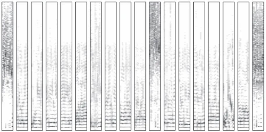
Figure 1.6 Dictionaries were learned from speech data of a given speaker. Shown are the
dictionaries learned for 18 of the 40 states. Each dictionary is comprised of 10 elements that are stacked next to each other. Each of these dictionaries roughly corresponds to a subunit of speech, either a voiced or unvoiced phoneme.
The notion of a state is incorporated in the NMF framework by associating distinct dictionary elements with each state. This is done by allowing each state to deter-mine a different support of the activations, which we express with the distribution p(h(n)| q(n)). This is to say that given a state, the model allows only certain dic-tionary elements to be active. Some techniques (Ozerov et al., 2009; Nakano et al., 2010) define the support of each state to be a single dictionary element, while other techniques (Mysore et al., 2010; Mysore and Smaragdis, 2011; Mohammadiha and Leijon, 2013), called non-negative HMMs (N-HMMs), allow the support of each state to be a number of dictionary elements. Since only a subset of the dictionary el-ements are active at each time frame (as determined by the state at that time frame), we can interpret these models as imposing block sparsity on the dictionary elements (Mysore, 2012).
As in (1.19), there is a dependency between h(n) and h(n 1). However, unlike the continuous models, this dependency is only through the hidden states, which are in turn related through the temporal dynamics. Therefore h(n) is conditionally independent of h(n 1) given q(n) or q(n 1). In the case of discrete models, we can therefore replace Eq. (1.19) with
q(n) ⇠ P (q(n) | q(n 1)) , (1.55)
h(n) ⇠ p (h(n) | q(n)) . (1.56)
Since these models incorporate an HMM structure into an NMF framework, one can make use of the vast theory of Markov chains to extend these models in various ways. For example, one can incorporate high level knowledge of a particular class of signals into the model, use higher order Markov chains, or use various natural language pro-cessing techniques. Language models were incorporated in this framework (Mysore
26
and Smaragdis, 2012) as typically done in the speech recognition literature (Rabiner, 1989). Similarly, one can incorporate other types of temporal structure like music theory rules when modeling music signals.
The above techniques discuss how to model a single source using an HMM struc-ture. However, in order to perform source separation, we need to model mixtures. This is typically done by combining the individual source models into a non-negative factorial HMM (N-FHMM). (Ozerov et al., 2009; Mysore et al., 2010; Mysore and Smaragdis, 2011; Nakano et al., 2011; Mohammadiha and Leijon, 2013), which al-lows each source to be governed by a distinct pattern of temporal dynamics. One issue with this strategy is that the computational complexity of inference is exponen-tial in the number of sources. This can be circumvented using approximate inference techniques such as variational inference (Mysore and Sahani, 2012), which makes the complexity linear in the number of sources.
1.5.2
A special case
We describe the specific N-HMM and N-FHMM models in (Mysore et al., 2010). A detailed derivation can be found in (Mysore, 2010). In the N-HMM, each state qcorresponds to a distinct dictionary, which is to say that a different subset of the dictionary elements in the model are associated with each state and we in turn call these subsets, dictionaries. There is therefore a one to one correspondence between states and dictionaries.
An example of the dictionaries learned from a sample of speech is shown in Fig. 1.6. Each dictionary in the figure is comprised of dictionary elements that are stacked next to each other. Notice the visual similarity of these dictionaries with the dictionary elements learned from convolutive NMF shown in Fig. 1.4. However, con-volutive NMF dictionaries are defined over multiple time frames, so they can only well model data that is of the same fixed length as the dictionaries. For example, they can model a drum hit quite well, but have less flexibility to model data such as phonemes of speech with varying lengths. On the other hand, N-HMMs model each time frame (with temporal dependencies between time frames) and therefore have more flexibility. They can model phonemes of speech of varying lengths quite well, but the increased flexibility comes with potential decreased accuracy for fixed length events such as a drum hit.
Similar to the dynamic NMF model in Section 1.4.2, the N-HMM is a dynamic extension of PLCA. We now briefly describe the model and parameter estimation for the N-HMM. The dictionary element k from dictionary (state) q is defined by a discrete distribution P (f|k, q), which shows the relative magnitude of the frequency bins for that dictionary element. It is by definition, time-invariant. At time n, the ac-tivations of dictionary element k from dictionary q is given by a discrete distribution P (k(n)|q(n)).
The complete set of distributions that form the N-HMM are defined below, and include the two distributions mentioned above. Each of these distributions except for the energy distributions are discrete distributions. The energy distributions are
Gaussian distributions.
1) Dictionary elements – P (f|k, q) defines the dictionary element k of dictionary q. Unlike the previous models that were discussed in this chapter, in the N-HMM, there is a grouping of the dictionary elements (columns of B). The B matrix is es-sentially a concatenation of the individual dictionaries of the N-HMM. Therefore, the dictionary q and dictionary element k together define a column of B. 2) Activations – P (k(n)|q(n)) defines the activations that correspond to dictionary
qat time n. The concatenation of these activations for all dictionaries weighted by the relative weighting of the individual dictionaries corresponds to h(n) given by P (h(n)|q(n)). This relative weighting at a given time frame is governed by the temporal dynamics mentioned below.
3) Transition matrix – P (q(n)|q(n 1)) defines a standard HMM transition matrix (Rabiner, 1989).
4) Prior probabilities – P (q(1)) defines a distribution over states at the first time frame.
5) Energy distributions – p(g(n)|q(n)) defines a distribution of the energies of state q, which intuitively corresponds to the range of observed loudness of each state. Given the spectrogram bV, of a sound source, we use the EM algorithm to learn the model parameters of the N-HMM. The E-step is computed as follows:
P (k(n), q(n)|f(n), bV, ) = P↵(q(n)) (q(n)) q(n)↵(q(n)) (q(n)) P (k(n)|f(n), q(n)) , (1.57) where P (k(n)|f(n), q(n)) = P P (k(n)|q(n))P (f(n)|k(n), q(n)) k(n)P (k(n)|q(n))P (f(n)|k(n), q(n)) . (1.58) P (k(n), q(n)|f(n), V, ) is the posterior distribution that is used to estimate the dictionary elements and activations. denotes the number of draws over each of the time frames in the spectrogram ( (1)... (N)). The number of draws in a given time frame intuitively corresponds to how loud the signal is at that time frame. The number of draws over all time frames is simply this information for the entire signal. Note that in spite of the dictionary elements P (f|k, q) being time invariant, they are given a time index n in the above equation. This is simply done in order to correspond to the values of f, k, and q referenced at time n in the LHS of the equation, and is constant for all values of n.
The forward/backward variables ↵(q(n)) and (q(n)) are computed using the likelihoods of the data, P (bv(n), g(n)|q(n)), for each state (as in classical HMMs
28
(Rabiner, 1989)). The likelihoods are computed as follows: p(bv(n), g(n)|q(n)) = p(g(n)|q(n))Y f (n) 0 @X k(n) P (f (n)|k(n), q(n))P (k(n)|q(n)) 1 A vf n , (1.59) where is scaling factor.
The dictionary elements and their weights are estimated in the M-step as follows: P (f|k, q) = P nvˆf nP (k(n), q(n)|f(n), bV, ) P f (n) P nvˆf nP (k(n), q(n)|f(n), bV, ) , (1.60) P (k(n)|q(n)) = P f (n)vˆf nP (k(n), q(n)|f(n), bV, ) P k(n) P f (n)ˆvf nP (k(n), q(n)|f(n), bV, ) . (1.61)
The transition matrix, P (q(n)|q(n 1)) and prior probability, P(q(1)), are com-puted exactly as in classical HMMs (Rabiner, 1989). The mean and variance of p(g|q) are also learned from the data.
N-HMMs are learned from isolated training data of sounds sources. Once these models are learned, they can be combined into an N-FHMM and used for source separation. If trained N-HMMs are available for all sources (e.g. separation of speech from multiple speakers), then supervised source separation can be performed (Mysore et al., 2010). This can be done efficiently using variational inference (Mysore and Sahani, 2012). If N-HMMs are available for all sources except for one (e.g. separation of speech and noise), then source separation can be performed using semi-supervised separation (Mysore and Smaragdis, 2011).
1.6
The use of dynamic models in source separation
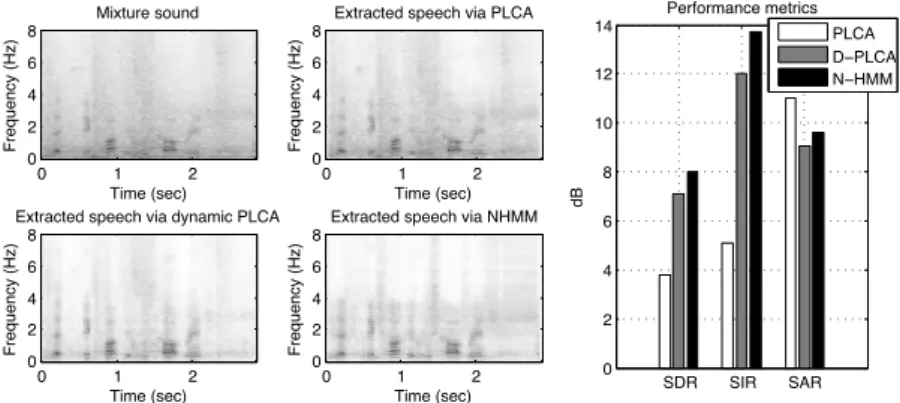
In order to demonstrate the utility of dynamic models in context, we use a real-world source separation example. This time it will be an acoustic mixture of speech mixed with background noise from a factory (using the TIMIT and NOISEX-92 databases). The mixture is shown using a magnitude STFT representation in Fig. 1.7. This partic-ular case is interesting because of the statistics of speech. We note that human speech tends to have a smooth acoustic trajectory which means that there is a strong tempo-ral correlation between adjacent time frames. On the other hand, we also know that speech has a strong discrete hidden structure which is associated with the sequence of spoken phonemes. These properties make this example a good candidate for demon-strating the differences between the methods discussed so far and their effects on source separation.
We performed source separation using the three main approaches that we covered in this chapter. These include a static PLCA model (Smaragdis et al., 2007), a dy-namic PLCA model (Mohammadiha et al., 2013) and an N-HMM (Mysore et al., 2010). In all three cases, we trained a model for speech and a model for background noise form training data. The dictionary size for the noise was fixed to 30 elements, whereas the speech model had 60 dictionary elements for PLCA and dynamic PLCA, and 40 states with 10 dictionary elements each for the N-HMM. For the dynamic models, we learned the temporal statistics as well. In order to separate a mixture of test data of the sources, we fixed the learned B matrices for both the speech and noise models and estimated their respective activations H using the context of each model. In figure 1.7, we show the reconstruction of speech using each model. We also show objective metrics using SDR, SIR, and SAR (defined in Chapter 1) to evaluate the quality of separation in each case. These results are averaged over 20 different speak-ers to reduce biasing and initialization effects.
For the static PLCA model, we see that there is a detectable amount of visible suppression of the background noise, which amounts to a modest SIR of about 5dB. The dynamic PLCA model on the other hand, by taking advantage of the temporal statistics of speech, does a much better job resulting in more than double the SIR. Note however that in the process of adhering to the expected statistics, it introduces artifacts, which result in a lower SAR as compared to the static model. The N-HMM results in an even higher SIR and a better SAR than the dynamic PLCA model. This is because the specific signal we are modeling has a temporal structure that is well de-scribed by a discrete dynamic model as we transition from phoneme to phoneme. By constraining our model to only use a small dictionary at each discrete state, we obtain a cleaner estimate of the source. An example of that can be seen when comparing the separation results in Fig. 1.7, where unwanted artifacts between the harmonics of speech in the dynamic PLCA example are not present in the N-HMM example since the dictionary elements within a state cannot produce such complex spectra.
1.7
Which model to use?
Now in addition to pondering on which cost function is the most appropriate to em-ploy, we also have a decision to make on which model is best for a source separation approach. As always the answer depends on the nature of the sources in the mixture. In general the static model has found success in a variety of areas, but does not take advantage of temporal correlations. In domains where we do not expect a high de-gree of correlations across time (e.g. short burst-like sources) this model works well, but in cases where we expect a strong sense of continuity (e.g. a smooth source like a whale song), then a continuous dynamic model would work better. Furthermore, if we know that a source exhibits a behavior of switching through different states, each with its own unique character (e.g. speech), then a model like the N-HMM is more appropriate since it will eliminate the concurrent use of elements that belong at different states and produce a more plausible reconstruction. Of course by using
30 Mixture sound Time (sec) Frequency (Hz) 0 1 2 0 2 4 6 8
Extracted speech via PLCA
Time (sec) Frequency (Hz) 0 1 2 0 2 4 6 8
Extracted speech via dynamic PLCA
Time (sec) Frequency (Hz) 0 1 2 0 2 4 6 8
Extracted speech via NHMM
Time (sec) Frequency (Hz) 0 1 2 0 2 4 6 8 SDR SIR SAR 0 2 4 6 8 10 12 14 dB Performance metrics PLCA D−PLCA N−HMM
Figure 1.7 Example of dynamic models for source separation. The four spectrograms
show the mixture, and the extracted speech for three different approaches. The bar plots shows a quantitative evaluation of the separation performance of each approach. Reproduced from (Smaragdis et al., 2014).
the generalized formulation we use in this article, there is nothing that limits us from employing different models concurrently. It is entirely plausible to design a source separation system where one source is modeled by a static model and other by a dy-namic one, or even have both being described by different kinds of dydy-namic models. Doing so usually requires a relatively straightforward application of the estimation process that we outlined earlier. Similarly, convolutive NMF can readily be employed together with any of the proposed models for H as the updates of these two variables are independent in the considered setting of alternate updates. This may efficiently combine the two sources of temporality in sound and further improve the precision of modeling.
1.8 Summary
In this chapter, we discussed several extensions of NMF where temporal dependen-cies are utilized to better separate individual speech sources from a given mixture signal. The main focus of this chapter has been on probabilistic formulations where temporal dependencies can be utilized to build informative prior distributions to be combined with appropriate probabilistic NMF formulations. The presented dynamic extensions are classified into continuous and discrete models, where both models are explained using a unified framework. The continuous models include smooth NMF and more recently proposed continuous state-space models. For the discrete mod-els, we discussed the discrete state-space models based on HMM, where the output distributions are modeled using static NMF. Short simulation results and qualitative comparisons are also provided to provide an insight into different models and their
performance. 1.9 Standard distributions Gamma distribution G(x|↵, ) = ↵ (↵)x ↵ 1exp( x), x 0 (1.62) mode(X) =↵ 1, E (X) = ↵, E ✓1 X ◆ = ↵ 1 (1.63) Exponential distribution E(x| ) = 1exp( x/ ), x 0 (1.64) E (X) = (1.65) inverse-Gamma distribution IG(x|↵, ) = ↵ (↵)x (↵+1) exp( x), x 0 (1.66) mode(X) = ↵ + 1, E (X) = ↵ 1, E ✓ 1 X ◆ =↵ (1.67) Multinomial M(x|N, p) =x N ! 1! . . . xK! px1 1 . . . p xK K , xk2 {0, . . . , N}, X k xk= N (1.68) Bibliography
Brown, J.C. (1991) Calculation of a constant q spectral transform. Journal of the Acoustical
Society of America, 89 (1), 425–434.
Cemgil, A.T. and Dikmen, O. (2007) Conjugate gamma Markov random fields for modelling nonstationary sources, in Proceedings of
International Conference on Independent Component Analysis and Signal Separation.
Chen, Z., Cichocki, A., and Rutkowski, T.M. (2006) Constrained non-negative matrix
factorization method for EEG analysis in early detection of Alzheimer’s disease, in
Proceedings of IEEE International Conference on Audio, Speech and Signal Processing.
Dempster, A.P., Laird, N.M., and Rubin., D.B. (1977) Maximum likelihood from incomplete data via the EM algorithm.
Journal of the Royal Statistical Society: Series B, 39, 1–38.
32
Dikmen, O. and Cemgil, A.T. (2010) Gamma Markov random fields for audio source modeling. IEEE Transactions on Audio,
Speech, and Language Processing, 18 (3),
589–601.
Essid, S. and Févotte (2013) Smooth nonnegative matrix factorization for unsupervised audiovisual document structuring. IEEE Transactions on
Multimedia, 15 (2), 415–425.
Févotte, C. (2011) Majorization-minimization algorithm for smooth Itakura-Saito nonnegative matrix factorization, in
Proceedings of IEEE International Conference on Audio, Speech and Signal Processing.
Févotte, C., Bertin, N., and Durrieu, J.L. (2009) Nonnegative matrix factorization with the Itakura-Saito divergence. With application to music analysis. Neural Computation,
21 (3), 793–830.
Févotte, C. and Idier, J. (2011) Algorithms for nonnegative matrix factorization with the beta-divergence. Neural Computation,
23 (9), 2421–2456.
Févotte, C., Le Roux, J., and Hershey, J.R. (2013) Non-negative dynamical system with application to speech and audio, in
Proceedings of IEEE International Conference on Audio, Speech and Signal Processing.
Hamilton, J.D. (1994) Time Series Analysis, Princeton University Press, New Jersey. Lütkepohl, H. (2005) New Introduction to
Multiple Time Series Analysis, Springer.
Mohammadiha, N. and Leijon, A. (2013) Nonnegative HMM for babble noise derived from speech HMM: Application to speech enhancement. IEEE Transactions on Audio,
Speech, and Language Processing, 21 (5),
998–1011.
Mohammadiha, N., Smaragdis, P., and Leijon, A. (2013) Prediction based filtering and smoothing to exploit temporal dependencies in NMF, in Proceedings of IEEE
International Conference on Audio, Speech and Signal Processing.
Mohammadiha, N., Smaragdis, P., Panahandeh, G., and Doclo, S. (2015) A state-space approach to dynamic nonnegative matrix factorization. IEEE Transactions on Signal
Processing, 63 (4), 949–959.
Mysore, G.J. (2010) A Non-negative
Framework for Joint Modeling of Spectral Structure and Temporal Dynamics in Sound Mixtures, Ph.D. thesis, Stanford University.
Mysore, G.J. (2012) A block sparsity approach to multiple dictionary learning for audio modeling, in Proceedings of International
Conference on Machine Learning Workshop on Sparsity, Dictionaries, and Projections in Machine Learning and Signal Processing.
Mysore, G.J. and Sahani, M. (2012) Variational inference in non-negative factorial hidden Markov models for efficient audio source separation, in Proceedings of International
Conference on Machine Learning.
Mysore, G.J. and Smaragdis, P. (2011) A non-negative approach to semi-supervised separation of speech from noise with the use of temporal dynamics, in Proceedings of
IEEE International Conference on Audio, Speech and Signal Processing.
Mysore, G.J. and Smaragdis, P. (2012) A non-negative approach to language informed speech separation, in Proceedings of
International Conference on Latent Variable Analysis and Signal Separation.
Mysore, G.J., Smaragdis, P., and Raj, B. (2010) Non-negative hidden Markov modeling of audio with application to source separation, in Proceedings of International Conference
on Latent Variable Analysis and Signal Separation.
Nakano, M., Le Roux, J., Kameoka, H., Nakamura, T., Ono, N., and Sagayama, S. (2011) Bayesian nonparametric spectrogram modeling based on infinite factorial infinite hidden Markov model, in Proceedings of
IEEE Workshop on Applications of Signal Processing to Audio and Acoustics.
Nakano, M., Roux, J.L., Kameoka, H., Kitano, Y., Ono, N., and Sagayama, S. (2010) Nonnegative matrix factorization with Markov-chained bases for modeling time-varying patterns in music spectrograms, in Proceedings of
International Conference on Latent Variable Analysis and Signal Separation.
Nam, J., Mysore, G.J., and Smaragdis, P. (2012) Sound recognition in mixtures, in
Proceedings of International Conference on Latent Variable Analysis and Signal Separation.
O’Grady, P.D. and Pearlmutter, B.A. (2008) Discovering speech phones using
convolutive non-negative matrix factorisation with a sparseness constraint.
Neurocomputing, 72, 88–101.
Ozerov, A., Févotte, C., and Charbit, M. (2009) Factorial scaled hidden Markov model for polyphonic audio representation and source separation, in Proceedings of IEEE
Workshop on Applications of Signal Processing to Audio and Acoustics.
Rabiner, L.R. (1989) A tutorial on hidden Markov models and selected applications in speech recognition. Proceedings of the
IEEE, 77 (2), 257–286.
Smaragdis, P. (2007) Convolutive speech bases and their application to supervised speech separation. IEEE Transactions on Audio,
Speech, and Language Processing, 15 (1),
1–12.
Smaragdis, P., Févotte, C., Mysore, G., Mohammadiha, N., and Hoffman, M. (2014) Static and dynamic source separation using nonnegative factorizations: A unified view.
IEEE Signal Processing Magazine, 31 (3),
66–75.
Smaragdis, P. and Raj, B. (2007) Shift-invariant probabilistic latent component analysis,
Tech. Rep. TR2007-009, Mitsubishi Electric
Research Labs.
Smaragdis, P., Raj, B., and Shashanka, M.V. (2006) A probabilistic latent variable model for acoustic modeling, in Proceedings of
Neural Information Processing Systems
Workshop on Advances in Models for Acoustic Processing.
Smaragdis, P., Raj, B., and Shashanka, M.V. (2007) Supervised and semi-supervised separation of sounds from single-channel mixtures, in Proceedings of International
Conference on Independent Component Analysis and Signal Separation.
Virtanen, T. (2007) Monaural sound source separation by non-negative matrix factorization with temporal continuity and sparseness criteria. IEEE Transactions on
Audio, Speech, and Language Processing,
15 (3), 1066–1074.
Virtanen, T., Cemgil, A.T., and Godsill, S. (2008) Bayesian extensions to non-negative matrix factorisation for audio signal modelling, in Proceedings of IEEE
International Conference on Audio, Speech and Signal Processing.
Wang, W., Cichocki, A., and Chambers, J.A. (2009) A multiplicative algorithm for convolutive non-negative matrix factorization based on squared Euclidean distance. IEEE Transactions on Signal
Processing, 57 (7), 2858–2864.
Yoshii, K. and Goto, M. (2012) Infinite composite autoregressive models for music signal analysis, in Proceedings of
International Society for Music Information Retrieval Conference.