A New Statistical Model for Random Unit Vectors
by
Karim Oualkacha & Louis-Paul Rivest Departement of Mathematics and Statistics
Universit´e Laval, Ste-Foy Qu´ebec
Canada G1K 7P4
Journal of Multivariate Analysis, 2008, doi:10.1016/j.jmva.2008.03.004
Abstract
This paper proposes a new statistical model for symmetric axial directional data in dimension p. This proposal is an alternative to the Bingham distribution and to the angular central Gaussian family. The statistical properties for this model are presented. An explicit form for its normalizing constant is given and some moments and limiting distributions are derived. The proposed density is shown to apply to the modeling of 3 × 3 rotation matrices by representing them as quaternions, which are unit vectors in <4. The moment estimators of
the parameters of the new model are calculated; explicit expressions for their sampling variances are given. The analysis of data measuring the posture of the right arm of subjects performing a drilling task illustrates the application of the proposed model.
Spherical symmetry; Quaternion; Rotation.
1
Introduction
This paper is motivated by the statistical analysis of samples of 3 × 3 ro-tation matrices. These matrices are used to characterize the orienro-tations of the limbs of human subjects or the posture of human joints in biomechanics. Recording a 3×3 rotation matrix typically involves two reference frames. The x, y, and z axes of the laboratory reference frame depend on the camera sys-tem making the measurements while the local axes are characteristics of the object being measured. When measuring the posture of a limb the local axes typically represent the flexion axis and the direction of the limb. Statistical models for 3 × 3 rotation matrices are useful to characterize the variability within a sample and to compare several samples of rotation matrices.
The main statistical model for rotation matrices is the exponential family of Downs (1972); some of its properties are reviewed in Khatri and Mardia (1977), Mardia and Jupp (2000) and Chikuse (2002). It has a complicated normalizing constant so that its moments and the maximum likelihood es-timator of its shape parameter are relatively difficult to evaluate. The sim-ulation of random rotations following Downs model is not simple. L´eon et al. (2006) proposed an alternative density that leads to relatively simple statistical procedures. Its high degree of symmetry makes it unsuitable for many of the samples of rotation matrices found in applications.
This paper constructs a model for 3 × 3 rotation matrices by proposing a new class of densities for axial unit vectors defined on Sp−1. The proposed
model applies to 3 × 3 rotation matrices since they can be represented as quaternions which are 4 × 1 unit vectors. Prentice (1986) and Rancourt, Rivest and Asselin (2000) use this representation.
The proposed density is an alternative to the exponential model of Bing-ham (1974), and to the angular central Gaussian family of Tyler (1987) which are reviewed in Section 9.4 of Mardia and Jupp (2000). Prentice (1986) noted that when a quaternion follows the Bingham distribution, the corresponding 3 × 3 rotation matrix has the matrix Fisher von Mises distribution. A distri-bution for 3 × 3 rotation matrices can be derived in a similar way from the angular Gaussian model.
Section 2 presents the new density in an arbitrary dimension p; it is parameterized by a vector of shape parameters γ ∈ <p−1 and M ∈ SO(p),
where SO(p) is the set of p × p rotation matrices. Random unit vectors distributed according to the proposed model are shown to be simple functions of independent random variables having beta distributions. Thus calculating moments and simulating vectors from the new distribution is simple. Section 3 studies the model in dimension 4 for the statistical analysis of a sample of quaternions representing 3 × 3 rotation matrices. Section 4 gives moment estimators for γ and M and derive their sampling distributions. Section 5 applies this methodology to the drilling data and suggests a goodness-of-fit test.
2
A General Model for Unsigned Unit
Direc-tions in S
p−1The proposed density with respect to the Lebesgue measure on Sp−1 is
gM,γ,p(r) = 1 cγ,p p−1 Y k=1 £Xk l=1 (MT l r)2 ¤γk−γk−1 r ∈ Sp−1,
where Sp−1 is the unit sphere in <p, M = (M
1, . . . , Mp) ∈ SO(p) is a p × p
rotation matrix, γ0 = 0, γ = (γ1, . . . , γp−1)T ∈ <p−1, with γp−1 > γp−2 >
. . . > γ1 > 0, cγ,p is the normalizing constant, and AT denotes the transpose
the of the matrix A. The constraint that all the γk’s are different ensures
that all the column of the matrix M are identifiable. When γk = γk+1 for
k < p − 1, one cannot distinguish Mk from Mk+1. Thus some elements
of the parameter M are not estimable. The proposed model is axial since gM,γ,p(r) = gM,γ,p(−r).
If r is distributed according to gM,γ,p, then u = MTr is distributed
ac-cording to gIp,γ,p. This is the density of the reduced model, denoted by gγ,p,
that is given by gγ,p(u) = [cγ,p]−1 p−1 Y k=1 £Xk l=1 u2 l ¤γk−γk−1 u = (u1, . . . , up)T ∈ Sp−1.(2.1)
The normalizing constant of this model has an explicit form. It is given in the following proposition. All the proofs appear in the Appendix.
Proposition 1: The normalizing constant is given by
cγ,p = 2(π) p−1 2 p−1 Y k=1 Γ(γk+k2) Γ(γk+k+12 ) .
If the γj’s are equal with γ1 = γ2 = . . . = γp−1 = γ, then the model
parameters are the unit vector M1 and a univariate shape parameter γ. The distribution of r is rotationally symmetric about M1; its density can be writ-ten as grs
M1,γ,p(r). The reduced model (2.1) becomes
grs γ,p(u) = Γ(γ + p2) 2(π)p−12 Γ(γ +1 2) u2γ1 , u ∈ Sp−1. (2.2)
If the common value of γ is 0, one gets the uniform distribution on Sp−1 and
c0,p = 2πp/2/Γ(p/2) is the Lebesgue measure of Sp−1. Observe however that, for any γ > 0, grs
γ,p(u) = 0 if u1 = 0. Thus as the shape vector goes to 0, gM,γ,p(r) does not converge uniformly to the uniform distribution. Following
Watson (1983, p. 92) one can show that the marginal distribution of u1, is grsγ (u1) = Γ(γ + p2) Γ(p−1 2 )Γ(γ + 1 2) u2γ1 (1 − u21)p−32 , u1 ∈ [−1, 1], that is u2
1follows a beta(γ+1/2, (p−1)/2) distribution and that (u2, . . . , up)T/
p 1 − u2 1 is uniformly distributed in Sp−2. When p = 2, (2.1) becomes gγ,2(u1, u2) = Γ(γ + 1) 2√πΓ(γ + 1 2) u2γ1 , (u1, u2)T ∈ S1. (2.3) This is related to the circular beta density with parameters (γ + 1/2, 1/2), see Jammalamadaka & SenGupta (2001, p. 51), whose density is given by
gγ,2(θ) =
Γ(γ + 1) 2γ+1√πΓ(γ + 1
2)
[1 + cos (θ)]γ, −π ≤ θ ≤ π.
If θ has this circular beta density, then u = (cos(θ/2), ² sin(θ/2))T is
The distribution of up, the last component of u, in (2.1) can be determined
using Watson’s (1983, p. 44) parametrization of Sp−1,
u = t 0 1 +√1 − t2 v 0 , t ∈ [−1, 1], v ∈ Sp−2,
whose Jacobian is du = (1 − t2)p−32 dtdv. Thus the joint density of (t, v) is
gγ,p(t, v) = [cγ,p−1]−1 p−2 Y k=1 " k X l=1 v2 l #γk−γk−1 Γ(γp−1+ p2) √ πΓ(γp−1+p−12 ) (1 − t2)γp−1+p−32 ,
where v ∈ Sp−2 and t ∈ [−1, 1]. Thus t and v are independent, the marginal
density of v is gγ,p−1(v), with γ = (γ1, γ2, . . . , γp−2)T, and the marginal
dis-tribution of t is given by fT(t) = Γ(γp−1+p2) √ πΓ(γp−1+ p−12 ) (1 − t2)(p−32 +γp−1), t ∈ [−1, 1].
This is the density function of (2βp−1−1), where βp−1is distributed according
to a beta(γp−1+ (p − 1)/2, γp−1+ (p − 1)/2). Hence, u satisfies
u =d 2 p βp−1(1 − βp−1)v (2βp−1− 1) ,
where = means equality in distribution. In a similar way, one can writed the distribution of the last entry of v in terms of a beta random variable. Iterating this procedure proves the following proposition.
Proposition 2: Let βj be independent random variables distributed
accord-ing to beta(γj + j/2, γj + j/2) distributions, for j = 1, . . . , p − 1 and let ²
the unit vector u = 2p−1Qp−1 1 p βj(1 − βj)² . . 2p−kQp−1 k p βj(1 − βj)(2βk−1− 1) . . (2βp−1− 1) p×1 , (2.4) is distributed according to gγ,p.
Proposition 2 shows that, starting from independent beta random vari-ables, a random vector distributed according to the proposed distribution is easily constructed. If we let u(k) = (u
1, . . . , uk)T, for k = 1, . . . , p, then from
(2.4), we can write u(k) as u(k)= c kv(k), (2.5) where ck = p u2 1+ . . . + u2k = 2p−k Qp−1 k p βj(1 − βj) and v(k) ∈ Sk−1. Since
ck is a function of βk, . . . , βp−1 and v(k) depends only on βk−1, . . . , β1, the random variable ckis independent of the unit vector v(k), which is distributed
according to gγ,k, with γ = (γ1, . . . , γk−1)T.
If in (2.4) we let yj = 4βj(1−βj), then one can show that yj is distributed
according to a beta(γj + j/2, 1/2). Thus an alternative form for (2.4) is
uk = Ãp−1 Y j=k √ yj ! p 1 − yk−1²k, k = 1, 2, . . . , p,
where ²k’s are random variables distributed according to the discrete uniform
2.1
Limiting Cases
This section derives limiting distributions obtained when some elements of the shape parameter vector γ go to infinity. The derivations rely on the following result. If γj = αjτ , then as τ goes to infinity,
√ τ (2βj− 1) −→d N µ 0, 1 2αj ¶ , q βj(1 − βj) prob −−→ 1 2,
where βj is distributed according to a beta(γj+ j/2, γj+ j/2). Together with
(2.4), these results can be used to derive the following limiting distribution.
Proposition 3: Suppose that γj is fixed, for j = 1, . . . , k − 1 and γj = αjτ ,
for j = k, . . . , p − 1, for some 1 ≤ k ≤ p. If u is distributed as gγ,p then, as
τ → ∞,
1. The limiting density of (u1, . . . , uk)T is gγ,k(.), with γ = (γ1, . . . , γk−1);
2. The vector√τ (uk+1, . . . , up)T converges in distribution to a Np−k
³
0, diag¡ 1 2αj
¢´ .
When k = 1, |u1| tends to 1 in probability and u is distributed in one of the two hyperplanes tangent to Sp−1 at (±1, 0, . . . , 0)T. When k > 1, the unit
vector u is distributed close to the subspace of Sp−1of dimension k−1 defined
by the equation u2
1+ . . . + u2k = 1. The distance between u and this subspace
is characterized by (uk+1, . . . , up)T that has a limiting normal distribution.
2.2
A Closure Property
Suppose that given x ∈ Sp−1, the random vector r has a rotationally
sym-metric density about x, grs
is uniformly distributed in a q dimensional subspace of Sp−1. Then x = Uv,
where U = (U1, . . . , Uq)p×q, p > q, UTU = Iq and v is uniform in Sq−1. The
marginal distribution of r is given by g(r) = Z Sq−1 Γ(γ + p/2)Γ(q/2) 4π(p+q−1)/2Γ(γ + 1/2)(r TUv)2γdv = ³√rTUUTr ´2γ Γ(γ + p/2)Γ(q/2) 4π(p+q−1)/2Γ(γ + 1/2) Z Sq−1 µ vTUTr √ rTUUTr ¶2γ dv = Γ(γ + p/2)Γ(q/2) 2πp/2Γ(γ + q/2) ( q X i=1 (UT i r)2 )γ .
This is the reduced model gγ∗,p(r) where the first q − 1 components of the
shape parameters γ∗ are equal to γ while its last p − q components are 0.
Such models are considered in Chapter 5 of Watson (1983). The competing models of Bingham and Tyler do not satisfy such a closure property.
2.3
Moment Calculations
The moments of the unit vector u distributed as gγ,p are given next. As
shown in the Appendix, they are derived from (2.4), by evaluating moments of beta random variables.
Proposition 4: Let u be distributed according to gγ,p(u), where the p − 1
entries of γ satisfy γp−1 > γp−2 > . . . > γ1 > 0; the matrix of second order moments of u is given by E(uuT) = diag(λ
k), where λk= E(u2k) is given by
λk = 1 2(γk−1+k2) p−1 Y j=k (γj +j2) (γj +j+12 ) and λ1 > λ2 > . . . > λp, and γ0 = 0. Moreover, E(u4 k) = 3 4(γk−1+ k2)(γk−1+k+22 ) p−1 Y j=k (γj +2j)(γj +j+22 ) (γj+ j+12 )(γj +j+32 ) ,
E(u2 ku2l) = 1 4(γk−1+k2)(γl−1+l+22 ) p−1 Y j=k (γj +j2) (γj +j+12 ) p−1 Y j=l (γj +j+22 ) (γj +j+32 ) , k < l, = λk 2(γl−1+l+22 ) p−1 Y j=l (γj +j+22 ) (γj +j+32 ) , k < l, (2.6)
E(uk) = E(ukul) = E(u3kul) = 0, k 6= l,
where the product is equal to 1 when k = p.
Let r = Mu, then the matrix of second order moments of r is given by E(rrT) = Mdiag(λ
1, . . . , λp)MT, (2.7)
where λ1 > . . . > λp > 0 are the eigenvalues of E(rrT). Furthermore the jth
column of M, Mj, is the eigenvector associated with λj.
3
The Model in the Special Case p = 4
When p = 4, gM,γ,p gives a model for quaternions, a representation of 3 × 3
rotation matrices. This section investigates the application of the proposed model to 3 × 3 rotation matrices. First, the correspondence between 3 × 3 ro-tation matrices and quaternions is reviewed in Section 3.1. To our knowledge p = 4 is the only instance of such a correspondance between unit vectors and rotation matrices.
3.1
3 × 3 Rotation Matrices and Quaternions
Let R(θ, µ) denote a rotation of angle θ, θ ∈ (−π, π], around the unit vector µ in <3. We have
R(θ, µ) = exp S(θµ) = I3+ S(θµ) + S(θµ)2/2 + ... = cos θI3+ sin θS(µ) + (1 − cos θ)µµt,
where S(µ) is the skew-symmetric matrix corresponding to µ = (µ1, µ2, µ3)T, given by S(µ) = 0 −µ3 µ2 µ3 0 −µ1 −µ2 µ1 0 .
The quaternion associated with R(θ, µ) is a unit vector in <4 defined by q(θ, µ) = (cos (θ/2), sin (θ/2)µT)T (Hamilton, 1969). Note that, q(θ, µ) =
−q(θ + 2π, µ), so that q and −q represent the same rotation. The rotation matrix R can be expressed in terms of its quaternion q as (Prentice, 1986),
R = Φ(q) = q2 1+ q22− q32− q24 2(q2q3− q1q4) 2(q1q3+ q2q4) 2(q1q4+ q2q3) q12+ q32− q22− q42 2(q3q4− q1q2) 2(q2q4− q3q1) 2(q3q4+ q1q2) q21 + q42− q22− q23 (3.1).
Quaternions are endowed with a special product corresponding to rotation multiplication. Let p and q be the quaternions for the rotation matrices R1 and R2respectively. As mentioned in McCarthy (1990, p. 61), the quaternion for the product R1R2 is the vector P+q = Q−p, where P+ and Q− are 4 × 4
rotation matrices defined by
and S+(x) = 0 −xT x S(x) , S−(x) = 0 −xT x −S(x) , x ∈ <3. Observe that tp = (p
1, −p2, −p3, −p4)T is the quaternion for the rotation matrix inverse of R1,RT1. Thus, P+Tq is the quaternion for RT1R2, moreover, PT
+q = Q−(tp).
Moran (1976) and Kim (1991) observed that if the rotation matrix R is distributed according to the uniform distribution in SO(3) then its quater-nion r is such that ²r is uniformly distributed on the unit sphere S3 where ² takes the values −1 and +1 with a probability of 1/2. Thus the jacobian of the transformation that maps the upper half sphere of S3 into SO(3) is 1.
Any 4 × 4 rotation matrix M = (Mij)1≤i,j≤4, can be written as the matrix product P+Q−, where P+ and Q− are derived from the quaternions p and q
as in (3.2). Given M, we can find p and q as follows p1 = 1 4 q A2 1 + A22+ A23+ [tr(M)]2, q1 = sign{tr(M)} 4 q B2 1 + B22+ B32+ [tr(M)]2, p2 p3 p4 = − 1 4q1 B1 B2 B3 , q2 q3 q4 = − 1 4p1 A1 A2 A3 ,
where sign(x) is -1 if x is negative and 1 otherwise and A1 = M12− M21− M34+ M43, A2 = M13− M31+ M24− M42, A3 = M14− M41− M23+ M32, B1 = M12− M21+ M34− M43, B2 = M13− M31− M24+ M42, B3 = M14− M41+ M23− M32.
These results are derived by noting that trP+Q−= 4p1q1and that q1S+(p2, p3, p4)+ p1S−(q2, q3, q4) is the skew-symmetric part of P+Q−.
3.2
Moment Calculations
Let r be a quaternion distributed according to gM,γ,4 and let R be the rotation
matrix associated to r. We have r = Mu, M ∈ SO(4). From Section 3.1, there exist two quaternions p and q such as r = P+Q−u = P+U+q, where U+ is a 4 × 4 rotation matrix, associated to u by (3.2). In terms of 3 × 3 rotation matrices, this relationship can be written as R = P U Q, where P = Φ(p), U = Φ(u) and Q = Φ(q), are the 3 × 3 rotation matrices associated to quaternions p, u and q respectively and Φ(.) is given in (3.1). Since u is distributed as gγ,p, equation (3.1) and Proposition 2 imply that E(U) is
a diagonal matrix whose elements can be expressed in term of the second moments λk of Proposition 4. Consequently, we can write
E(R) = P E(U)Q = P diag λ1+ λ2− λ3− λ4 λ1+ λ3− λ2− λ4 λ1+ λ4− λ2− λ3 Q,
see also Section 4 of Prentice (1986). This is the singular value decomposition for E(R). The fact that λ1 ≥ . . . ≥ λ4 ≥ 0 implies that its singular values satisfy E(U11) > E(U22) > |E(U33)|. We conclude that the mean rotation is P Q see (Rivest, Rancourt, and Asselin 2000). The corresponding quaternion is P+q = M1, where M1 is the first column of the 4 × 4 rotation matrix M. This is the eigenvector associated to the largest eigenvalue λ1 of E(rrT).
When γ1 = γ2 = γ3 = γ, the reduced model in (2.1) becomes gsrγ,4(u)
given in (2.2). Using the transformation U = Φ(u) given in (3.1), that has the Jacobian [dU] = du/(2π2) where [dU] is the unit invariant measure on SO(3). One can write (2.1) in terms of 3 × 3 rotation matrices as
gγ(U) = √ πΓ(γ + 2) 22γΓ(γ + 1 2) [1 + tr(U)]γ.
This is equal to the model of Le´on, Rivest and Mass´e (2006) when p = 3.
3.3
A Great Circle Model
When modeling rotational data it may happen that λ3 and λ4 are very close to 0. For these models, γ2 and γ3 are large and the unit vector r takes its value in a great circle of S3. In this case, the standardized quaternion u satisfies u ≈ (u1, u2, 0, 0)T, where (u1, u2)T ∼ gγ,2(u1, u2), see (2.3). Thus
r = Mu can be written as r ≈ cos(θ/2)M1 + sin(θ/2)M2 = [M1]+ © cos(θ/2)(1, 0, 0, 0)T + sin(θ/2)[M1]T+M2 ª ,
where θ has a circular beta distribution with parameters (γ + 1/2, 1/2). One has [M1]T+M2 = (0, µT)T, where µ is a S2vector since [M1]T+M2is a unit vector
in <4 whose first component is null. In terms of 3 × 3 rotation matrices, the above expression for r is R = R0R(θ, µ), where R0 is the rotation matrix corresponding to M1 and R(θ, µ) is the rotation matrix corresponding to the quaternion (cos θ/2, sin θ/2µT)T. This is a situation where the variability in
R can be expressed as rotations around a fixed axis µ; the rotation angles have a circular beta distribution when r is distributed according to gM,γ,4.
From a geometrical point of view, µ is the rotation axis in the so called local reference frame. An alternative expression for the fixed axis model, with respect to the rotation axis R0µ in the laboratory reference frame, is R = R(θ, R0µ)R0. Fixed axis models for rotation matrices are investigated in Rivest (2001).
4
Parameter Estimation
Consider {r1, r2, . . . , rn}, a sample of unit vectors in <pdistributed according
to gM,γ,p(r), where γ ∈ <
p−1 and M ∈ SO(p) are unknown parameters. This
section discusses the estimation of γ and M. Moment estimators for γ and M which are functions of the sample cross-product matrixPrirTi /n are derived;
their asymptotic distributions are calculated.
This section emphasizes the method of moments to estimate parameters because it is simple and it has a large efficiency. The information matrix for the parameters of γ and M when p = 4, is given in Oualkacha (2004, Section 4.3). It shows that the efficiency of the moment estimators of γ and M is greater than 90% when the components of γ are relatively large, i. e. (γ1 > 2, γ2 > 4). For the rotationally symmetric models, the efficiency of
the moment estimators is calculated in section 5.2 of Le´on Rivest and Mass´e (2006), it is greater than 90% when γ > 4. This suggests that the lost of information associated with the moment estimators is small, especially when the data is clustered around its first principal direction.
4.1
Moment Estimators
The estimating equation for (M, γ) is ˆB = E(rrT), where E(rrT) is given
in (2.7) and ˆB =Pni rirTi /n. The matrix ˆB is positive definite; its spectral
decomposition is ˆ B = 1 n n X i rirTi = ˆM £ diag(ˆλj) ¤ 1≤j≤pMˆ T, (4.1)
where ˆM = ( ˆM1, ˆM2, . . . , ˆMp) is a matrix of eigenvectors associated to the
eigenvalues ˆλ1 > ˆλ2 > . . . > ˆλp. Consequently, the moment estimator of M
is ˆM and the moment estimator of γ, ˆγ, is defined implicitly by the equations ˆ
λj = λj, for j = 1, . . . , p, when λj is defined in Proposition 4. The solution
to these equations is ˆ γk = 1 2 ¡Pkj=1λˆj ˆ λk+1 − k¢, k = 1, 2, . . . , p − 1.
These moment estimates satisfy ˆγk+1 = ˆγkˆλk+1/ˆλk+2+(k+1)(ˆλk+1−ˆλk+2)/(2ˆλk+2).
This implies that ˆγ1 < ˆγ2 < . . . < ˆγp−1.
The asymptotic distributions of ˆγ and ˆM are now derived. For this, let m = vect(mjk)1≤j<k≤p a vector in <(p−1)p/2 close to zero, so
M exp¡S(m)¢ = M(Ip+ S(m) +
S(m)2
2! + · · · ) = M(Ip+ S(m) + o(m))
describes the rotation about M , where S(m) is a p×p skew-symmetric matrix containing the entries of m, such that S(m)jk = mjk for 1 ≤ j < k ≤ p. Thus
MTM = Iˆ
p+ S( ˆm), (4.2)
where ˆm = vect( ˆmjk)1≤j<k≤p measures the discrepancy between M and ˆM. The asymptotic distributions of ˆγ and ˆM are given in the next proposition which is proved in Appendix.
Proposition 5: As the sample size n becomes large, we have i) n1/2¡ˆγ − γ¢ → N
p−1(0p−1, Σγ),
where Σγ is a (p − 1) × (p − 1) diagonal matrix whose diagonal entries are
given by Σγ(k, k) = (γk+ k2)(γk+k+12 ) λk+1(γk+k+32 ) p−1 Y j=k+1 (γj +j+22 ) (γj +j+32 ) ,
where the product is equal to 1 when k = p − 1. ii) n1/2m → Nˆ (p−1)p 2 (0 (p−1)p 2 , Σm), where Σm = diag © Σmkl ª (p−1)p 2 × (p−1)p 2 , 1 ≤ k < l ≤ p,
where Σmkl is the variance of the component ˆmkl of ˆm that is given by
Σmkl = λk 2(λl− λk)2(γl−1+l+22 ) p−1 Y j=l (γj+ j+22 ) (γj+ j+32 ) , 1 ≤ k < l ≤ p.
The small sample biases of the asymptotic variances given in the above proposition have been investigated in a Monte-Carlo study that is not re-ported here. When n ≥ 50 ˆΣj(k, k)/ˆλ2k provides reliable variance estimates
for log ˆλk, where ˆΣj(k, k) is the plug-in variance estimate. The variance
es-timates obtained from Proposition 5 ii) also have small biases when n ≥ 50. For small sample sizes, the parametric bootstrap can be used to estimate the variances.
4.2
Estimation of the fixed axis model when p = 4
When p = 4 and when γ2 and γ3 are large, one has a fixed-axis model for the 3 × 3 rotation matrices as discussed in Section 3.3. This axis is estimated by ˆµ, the vector of the second, the third and the fourth entries of [ ˆM1]T+Mˆ2. The asymptotic distribution of ˆµ is given next.Proposition 6: As the sample size n becomes large, we have n1/2¡µ − µˆ ¢ → N3(0, Σµ), where Σµ is given by Σµ= £ Σm23 + Σm14 ¤ µ1µT1 + £ Σm13 + Σm24 ¤ µ2µT2, where (0, µT 1)T = [M1]T+M3 and (0, µT2)T = [M1]T+M4.
When γ2 and γ3 are large a convenient expression for this covariance matrix is Σµ= ½ λ3 λ2 +λ4 λ1 ¾ µ1µT1 + ½ λ4 λ2 + λ3 λ1 ¾ µ2µT2 + o( 1 γ2 ).
When γ2 = γ3, λ3 = λ4 and this expression coincides with the variance estimate given in Section 4.1 of Rivest (2001).
5
Data analysis
To illustrate the methodology presented in this paper, we fit the proposed model to the data collected from the experiment given in Rancourt et al. (2000). The sample consists of n = 30 observations that measure the orien-tations of the upper right arm of a subject performing drilling tasks. The arm pose is defined via one marker attached in the arm. The marker orien-tation is characterized by a 3 × 3 roorien-tation matrix R = [µx, µy, µz], where µx,
µy and µz are the orientations of the local’s x, y and z axes of the marker
in the laboratory coordinate system. When resting, the arm is in a vertical position, the local x axis then points backward, the local y axis goes upward and the local z axis points left. Thus the local y-axis is the direction of the upper arm, and the local z-axis is the rotation axis of the elbow. The subject is asked to point a drill at various targets 30 times. The rotation matrices in the sample record the orientations of the local coordinate system at each repetition. The n = 30 quaternions for the sample 3 × 3 rotation matrices are given in Table 1.
The moment estimators of log γj’s and their parametric bootstrap
stan-dard errors are log ˆγ1 = 2.60 s.e. = 0.28, log ˆγ2 = 5.35 s.e. = 0.28, and log ˆγ3 = 8.10 s.e. = 0.31. The large sample standard errors derived from Proposition 5 are 10% to 20% smaller than those obtained with the para-metric bootstrap. Since the ˆγ2 and ˆγ3 are large we have a fixed axis model. Thus Ri = ˆR0R(θi, ˆµ) and the variability of Ri in the local coordinate system
is characterized by θi that has a circular beta distribution with parameters
(ˆγ1+1/2, 1/2) around the fixed axis ˆµ. Since ˆγ1 = 13.42, the range of possible values for θi ±40 degrees, with a probability of 95%.
ri ri1 ri2 ri3 ri4 r1 0.664 0.193 0.390 -0.608 r2 -0.623 -0.167 -0.416 0.640 r3 -0.605 -0.195 -0.425 0.644 r4 -0.602 -0.178 -0.416 0.657 r5 -0.562 -0.276 -0.480 0.614 r6 0.791 0.098 0.369 -0.477 r7 0.802 0.056 0.391 -0.448 r8 0.755 0.098 0.381 -0.525 r9 0.789 0.079 0.371 -0.483 r10 0.732 0.109 0.393 -0.545 r11 0.859 0.067 0.395 -0.318 r12 0.853 0.042 0.372 -0.364 r13 0.866 0.023 0.364 -0.341 r14 0.829 0.033 0.366 -0.421 r15 0.852 0.054 0.361 -0.374 ri ri1 ri2 ri3 ri4 r16 0.920 0.059 0.368 -0.123 r17 0.895 0.034 0.360 -0.260 r18 0.910 0.050 0.378 -0.170 r19 0.916 0.043 0.355 -0.181 r20 0.926 0.008 0.333 -0.178 r21 0.795 0.053 0.386 -0.464 r22 0.780 0.042 0.344 -0.521 r23 0.772 0.064 0.355 -0.523 r24 0.791 0.016 0.352 -0.500 r25 0.701 0.104 0.383 -0.593 r26 0.876 0.009 0.349 -0.332 r27 0.850 0.045 0.358 -0.383 r28 0.837 0.039 0.380 -0.391 r29 0.898 0.005 0.334 -0.285 r30 0.874 0.055 0.351 -0.330 Table 1: Sample of n = 30 quaternions for the right arm pose in a drilling task.
The moment estimator of M1 is ˆM11 = 0.813 s.e. = 0.017, ˆM12 = 0.077 s.e. = 0.011, ˆM13 = 0.383 s.e. = 0.006 and ˆM14− 0.431 s.e. = 0.027, while the moment estimator of the fixed axis is ˆµ1 = −0.524 s.e. = .019,
ˆ
µ2 = −0.365 s.e. = .043, and ˆµ3 = 0.773 s.e. = .029. These standard errors were evaluated using the parametric bootstrap. Since the largest entry of ˆµ is the third one, the arm changes its posture by moving about an axis closed
to the z-axis. From Proposition 2, the angle of the residual rotation not explained by the fixed axis model has an N{0, (2ˆγ2)−1} distribution. The standard deviations is 3.9 degrees; this highlights that the residual rotation is small.
To interpret this analysis one must bear in mind that a change of the orientation of the upper arm is the composition of a rotation of the back plus a motion of the shoulder. For the subject considered here, the back did not move much since the analysis of the rotation data obtained from the back marker gives ˆγ1 = 113, s.e. = 29. Most of the changes in orientation take place at the shoulder joint. The changes in the posture of this joint occur mostly through rotations about ˆµ which is relatively close to the z axis. During the experiment the upper arm stays in a plane close to the z = 0 plane that is spanned by the x (backward direction) and the y (upward direction) axis.
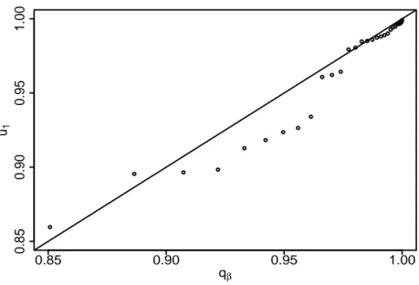
We now investigate the fit of the model. Since ˆγ2and ˆγ3are large, the cen-tered quaternions satisfy ui ≈ (cos(θi/2), sin(θi/2), 0, 0)T, where cos2(θi/2) is
distributed according to a beta(ˆγ1 + 1/2, 1/2). A goodness of fit test for the proposed distribution amounts to testing whether {cos2(θ
i/2)} has a
beta(ˆγ1 + 1/2, 1/2) distribution. First note that cos2(θi/2) is estimated by
( ˆM1ri)2; the beta(ˆγ1+ 1/2, 1/2) Q-Q plot is given in Figure 1.
The beta distribution fits reasonably well. To carry out formal good-ness of fit tests, we use the correlation coefficient in the Q-Q plot and the Kolmogorov-Smirnov statistic. The observed value for these two statistics are 0.967 and 0.157 respectively. To calculate p-values, we use the parametric bootstrap. The sampling distributions of these statistics are approximated by
0.85 0.90 0.95 1.00 0.85 0.90 0.95 1.00 qβ u1
Figure 1: Q-Q plot for the fit of the beta(ˆγ1 + 1/2, 1/2) distribution to the sample {( ˆMt
1ri)2}.
evaluating them repeatedly on data simulated from the proposed distribution with parameters equal to their moment estimates. The bootstrap p-values are 0.244 for the correlation test and 0.09 for the Kolmogorov-Smirnov test. The proposed model provides a reasonable fit.
6
Discussion
This paper has proposed a flexible model for axial data of arbitrary dimen-sion. The proposed density is well suited to analyze samples of 3 × 3 rotation matrices. Simple moments estimators of the parameters are available and
the simulation of data from the proposed distribution is simple making the parametric bootstrap an appealing strategy to determine the sampling dis-tributions of interest.
Appendix A
A.1. Proof of Proposition 1. We prove this proposition by induction. We can verify easily that for p = 2, cγ,2 is given by (2.3), now suppose that
proposition 1 true for p − 1. Using Watson’s (1983, p. 44) parametrization of Sp−1 given in Section 2, we have
cγ,p = Z v∈Sp−2 p−2 Y k=1 " k X l=1 v2 l #γk−γk−1 dv Z 1 −1 (1 − t2)γp−1+p−32 dt = cγ(p−1) √ πΓ(γp−1+ p−12 ) Γ(γp−1+p2) = 2(π)p−22 p−2 Y k=1 Γ(γk+ k2) Γ(γk+ k+12 ) √ πΓ(γp−1+p−12 ) Γ(γp−1+ p2) . This completes the proof of Proposition 1.
A.2. Proof of Proposition 4. The expressions for λk, E(u4k) and E(u2ku2l), 1 ≤
k < l ≤ p come from the decomposition of u as a product of beta random variables given in Proposition 2. They are derived by noting that if X is distributed as a β(γ + k/2, γ + k/2) random variable, then
4E{X(1 − X)} = γ + k/2 γ + (k + 1)/2, E{(2X − 1) 2} = 1 2{γ + (k + 1)/2}, 16E{X2(1 − X)2} = (γ + k/2)(γ + 1 + k/2) {γ + (k + 1)/2}{γ + (k + 3)/2}, E{(2X − 1)4} = 3 4(γ + k/2)(γ + 1 + k/2).
A.3. Proof of Proposition 5. Following Bellman (1970, chapter 4), one can write ˆ λj − λj = 1 n n X i=1 £ (MT j ri)2− λj ¤ + Op( 1 n) = 1 n n X i=1 u2 jiλj + Op( 1 n), and ˆ Mj− Mj = p X k6=j " 1 n n X i=1 MT j rirTi Mk λj− λk # Mk+ Op( 1 n) = p X k6=j " 1 n n X i=1 ujiuki λj− λk # Mk+ Op(1 n),
where uji is the j th component of the i th centered observation ui. Now let
³
∂ ∂ˆλγˆ
´ ¯
¯λ=λˆ the partial derivative (p − 1) × p matrix of ˆγ with respect to ˆλ at point λ = (λ1, . . . , λp)t. The kth row of the matrix is
1 λk+1 , . . . , 1 λk+1 | {z } k times , − Pk j=1λj λ2 k+1 , 0, . . . , 0 .
According to Slutzky’s theorem and to the central limit theorem, as n goes to infinity, ˆγ and ˆM have asymptotic normal distributions. Now we prove that the off diagonal terms of Σγ are zero (i.e: Σγ(k, l) = 0, k < l). To do so,
we can verify that
Σγ(p)(k, l) = 1 4E "µ ∂ ∂ˆλˆγ ¶ ¯ ¯λ=λˆ uuT µ ∂ ∂ˆλˆγ ¶T ¯ ¯ˆλ=λ # (k,l) = 1 4E "à u2 1+ . . . + u2k λk+1 − Pk j=1λju2k+1 λ2 k+1 ! à u2 1+ . . . + u2l λl+1 − Pl j=1λju2l+1 λ2 l+1 !# .
Using (2.5), the vector u(k+1) of the first k + 1 entries of u can be expressed as u(k+1) = (u2
1+ . . . + u2k+1)v(k+1), where v(k+1) is a random Sp vector. Thus
Σγ(k, l) becomes Σγ(p)(k, l) = 1 4E " ( v2 1 + . . . + vk2 λk+1 − Pk j=1λjvk+12 λ2 k+1 ) × ( (u2 1+ . . . + u2k+1) ÃPl j=1u2j λl+1 − Pl j=1λju2l+1 λ2 l+1 !) # .
The expectation on the right hand side involves the product of two random variables. The first one is a function of the (k + 1) × 1 unit vector v with distribution gγ,k+1. Considering Proposition 4, this first term has a null
expectation. In terms of the beta random variables defined in Proposition 2, the second term depends on βk+1, . . . , βp−1; it is therefore independent of
the first term. The diagonal terms of this matrix are evaluated using the following expression, Σγ(p)(k, k) = 1 4λ4 k+1 E{(u2 1+ . . . + u2k+1)2}E{(λk+1− v2k+1 k+1 X 1 λj)2}.
The variance covariance matrix for ˆM comes from (2.6). To prove iii) and that Σm is diagonal, observe that E(ujiu3ki) = E(ujiukiu2li) = 0, for all
j 6= k 6= l.
A.4. Proof of Proposition 6. It is derived immediately from (4.2), since [ ˆM1]+ and ˆM2 can be written as
[ ˆM1]T+ = [M1]T+− ˆm12[M2] T +− ˆm13[M3] T +− ˆm14[M4] T +, ˆ M2 = M2+ ˆm12M1− ˆm23M3− ˆm24M4.
Proposition 2 in Rivest (2001) shows that [M1]T+M3 = [M4]+TM2and [M3]T+M2 = [M1]T+M4. A first order expansion of [ ˆM1]T+Mˆ2 yields
0 ˆ µ − µ = − ( ˆm23 + ˆm14) [M1] T +M3− ( ˆm13+ ˆm24) [M1] T +M4+ op( ˆm 0 ˆ m). References
Bellman, R. (1970). Introduction to Matrix Analysis, 2nd ed. McGraw-Hill, New York
Bingham, C. (1974). An antipodally symmetric distribution on the sphere. Ann. Statist., 2, 1201-1225.
Chikuse, Y. (2002). Statistics on Special Manifolds. Springer-Verlag, New York.
Downs, T. D. (1972). Orientation statistics. Biometrika. 59, 665-676. Jammalamadaka, S. R. and SenGupta, A. (2001). Topics in Circular
Statis-tics. World Scientific Publishing Co. Pte. Ltd. London.
Khatri, C. G. and Mardia, K. V. (1977). The von Mises-Fisher distribution in orientation statistics. J. R. Statist. Soc. B 39, 95-106.
Kim, P.T. (1991). Decision theoretic analysis of spherical regression. Jour-nal of Multivariate AJour-nalysis. 38, 233-240
Le´on, C. A. , Mass´e, J. C. and Rivest, L. P. (2006). A statistical model for random rotations in SO(p). Journal of Multivariate Analysis. 97, 412-430.
Mardia, K. V. and Jupp, P. E. (2000). Directional Statistics. New York: John Wiley.
Moran, P.A.P. (1976). Quaternions, Haar measure and the estimation of a paleomagnetic rotation. In Perspsectives in Probability and Statistics (J. Gani, Ed.), pp. 295-301. Applied Probability Trust and Academic Press, London.
Oualkacha, K. (2004) ´Etude d’un mod`ele statistique pour les rotations. M´emoire pour l’obtention du grade de maˆıtre ´es sciences. Qu´ebec: Universit´e Laval.
Prentice, M. J. (1986). Orientation statistics without parametric assump-tions. J. R. Statist. Soc. B 48, 214-222
Rancourt, D., Rivest, L. P. and Asselin, J. (2000). Using orientation statis-tics to investigate variations in human kinemastatis-tics. Journal of the Royal Statistical Society Series C-Applied Statistics, 49, 81-94 .
Rivest, L. P. (2001). A directional model for the statistical analysis of movement in three dimensions. Biometrika. 88, 3, pp. 779-791. Watson, G. S. (1983). Statistics on Spheres. A Wiley-Interscience