ABSTRACT: The paper is concerned with the seismic analysis of large reservoirs. During an earthquake, it is known that the acceleration of the water contained in the reservoir produces an additional hydrodynamic pressure, which has a convective, a rigid and a flexible impulsive part. The two first contributions are already well-known and may therefore be easily integrated during a pre-design phase, but it is much more complicated to assess the flexible contribution, as it is influenced by the coupling between the structure and the fluid. The only consistent way seems to resort to finite elements methods, which are not always convenient at an early design stage. For this reason, some research have been undertaken to rapidly evaluate the flexible pressure acting on thick plates. The results obtained by using this simplified method have been compared to numerical solutions. The agreement was found to be quite satisfactory.
KEY WORDS: Dynamic pressure; Seismic structural response; Modal analysis; Fluid structure interaction.
1 INTRODUCTION
When a reservoir is submitted to an earthquake, it is well known that an additional hydrodynamic pressure is applied on the tank walls, because of the acceleration of the water that is confined in the chamber. This pressure has the three following contributions:
• The convective one, which is produced by the waves occurring at the free surface during the seismic excitation. This phenomenon is also called sloshing.
• The rigid impulsive one, which is derived under the assumption that the walls are perfectly rigid and move in unison with the ground.
• The flexible impulsive one, coming from the accelerations of the walls as an imperfectly rigid structures.
The two first parts may be easily characterized by some analytical formulae already available in the literature. Many solutions were proposed by various authors, such as Epstein [1], Haroun [2], Housner [3] or Ibrahim [4] amongst others. It is therefore quite easy to account for these forces when designing new gates. Moreover, as we are presently dealing with quite large reservoirs, the convective part is negligible in comparison with the two remaining ones, so it will not be considered any longer in this study.
Assessing the third contribution is a more arduous task. In fact, the pressure field is influenced by the proper accelerations of the walls, which, in turn, has an effect on the dynamic response of the structure itself. In other words, we are facing a coupled problem. This one may be solved by resorting to finite elements analyses, where both the fluid and the structure have to be modeled. However, such an approach may be time demanding, because developing a complete and consistent numerical representation of the liquid is not so
easy. Moreover, modeling entirely the fluid domain may lead to excessively long calculation times. Of course, this way of working is definitely not acceptable at an early stage of design, when engineers do not necessarily have a lot of time to perform fastidious calculations. Such an approach is also not conceivable when a great amount of scenarios or configurations have to be checked.
For all these reasons, it is quite clear that an alternative approach is necessary, as integrating the seismic action in the pre-design is of prior importance in regions frequently submitted to earthquakes. Nevertheless, developing an efficient simplified analytical procedure is not so easy, but we propose to go one step further in this paper by considering a large flexible reservoir undergoing a seismic acceleration.
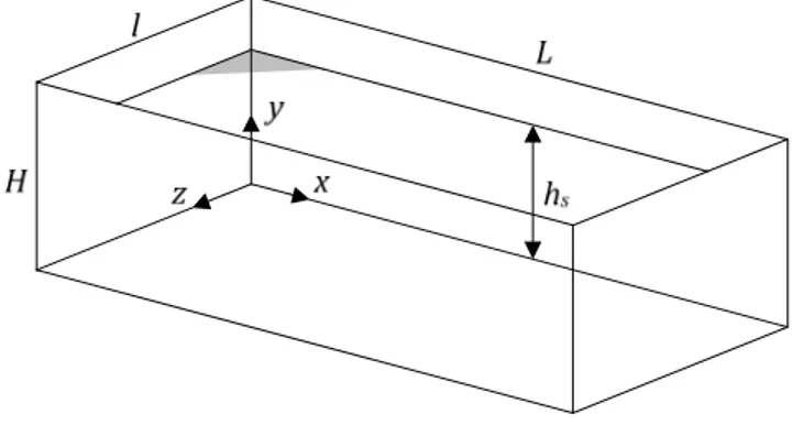
Figure 1. Flexible reservoir.
The tank under consideration here is depicted on Figure 1. It has a total length L, a width l and a height H. It is filled with water until the level hs and is submitted to a longitudinal acceleration Ẍ(t) acting along the x axis. The lateral walls located in z = 0 and z = l are considered to be perfectly rigid.
A Simplified procedure to assess the dynamic pressures on large reservoirs
L. Buldgen1, H. Degée2, H. Le Sourne3, P. Rigo2
1 FRIA PhD Student, Department of Structural Engineering, Faculty of Applied Sciences, University of Liège, Chemin des Chevreuils 1, 4000 Liège, Belgium
2
Department of Structural Engineering, Faculty of Applied Sciences, University of Liège, Chemin des Chevreuils 1, 4000 Liège, Belgium
3 Institut Catholique d'Arts et Métiers (ICAM), Avenue du Champ de Manoeuvres 35, 44470 Carquefou, France Emails: [email protected], [email protected], [email protected], [email protected]
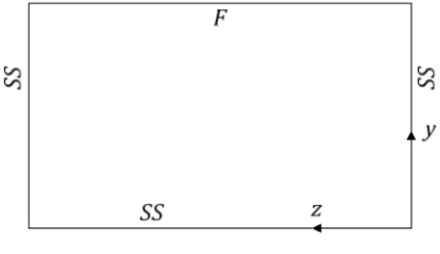
This is also the case for the ground located at y = 0. On the contrary, the walls at x = 0 and x = L are assumed to behave like a flexible plate simply supported on three edges (SS) and free at the upper one (F), as represented on Figure 2.
Figure 2. Boundary conditions.
2 FREE VIBRATION ANALYSIS OF A DRY PLATE In this section, we consider the free vibrations of the isotropic and homogenous plate depicted on Figure 2. The plate is made of a linear elastic material characterized by a density ρ, a Young modulus E and a Poisson ratio ν. The out-of-plane displacements along the x axis are denoted by u(y,z,t).
Under the hypothesis of small strains, one may apply the classical thin plates theory of Kirchhoff, in which the structural equilibrium may be expressed as:
(
)
(
X u)
D u p t p z u z y u y u D u X t p p − = ∇ + + ⇔ − = ∂ ∂ + ∂ ∂ ∂ + ∂ ∂ + + 4 4 4 2 2 4 4 4 2 & & & & & & & &ρ
ρ
(1)where tp and D are respectively the thickness and flexural rigidity of the plate. In equation (1), p denotes the total hydrodynamic pressure applied on the structure.
In order to derive the vibration properties for the dry plate, one can consider the homogenous form of equation (1), in which p and Ẍ are set to zero. In this case, the proper displacements have a sinusoidal form:
( )
1 sin ) , ( ) , , (y z t = y z t i≥ ui δi ωi (2)in which ωi and δi are known as the dry eigenfrequencies and mode shapes. Introducing (2) in (1) and applying the developments of Leissa [5] leads to:
(
)
(
1)
tan( )
tanh( )
0 1 2 2 2 2 2 = − + − − − H H c c i i i i i i i iλ
λ
λ
λ
ν
γ
ν
γ
(3)where ci is a function of ωi that has to be determined by solving (3). All the other parameters are defined hereafter:
D t c l n c ci i i i i i i i i p i 2 4 2 2 2 2 2 2
π
ρω
γ
γ
λ
γ
λ
= + = − = = (4)with ni = 1, 2, ... Furthermore, as shown by [5], the dry mode shapes δi are given by:
( )
( )
z l y B l y A z y i i i i i iγ
λ
λ
δ
, sin sinh sin − = (5)
where Ai is the modal amplitude and Bi is related to the other variables by:
( )
( )
( )
( )
H H c c B i i i i i i iλ
λ
ν
γ
ν
γ
sinh sin 1 1 2 2 2 2 + − − − = (6)It is worth bearing in mind that all the solutions detailed here above are only valid for a dry plate that is not in contact with water. In the present case however, the reservoir is filled up to a level hs, which means that equations (3) and (5) are not the vibration properties characterizing the wet plate. To account for the presence of a fluid, we first need to have a better characterization of the hydrodynamic pressure term p appearing in equation (1).
3 FREE VIBRATION ANALYSIS OF A WET PLATE 3.1 Characterization of the hydrodynamic pressure As recalled previously, a lot of analytical solutions are already available in the literature to evaluate the rigid impulsive pressure pr. One may consider, amongst others, the expression proposed by Kim et al. [6]:
( )
(
)
L X h y L p n n s n n f r ⋅&& − − =∑
+∞ =1 2 cosh 2 cosh 4β
β
β
ρ
(7)where βn = (2n − 1)π/L and ρf is the density of the fluid. On the other hand, if we still use the developments described by Rajalingham [7], the flexible impulsive contribution pf can be derived from:
( ) ( )
∑∑ ∫∫
+∞ = ∞ + = ⋅ ⋅ − = 1 0 0 0 cos cos n m h l m n mn f s dydz z y u C p &&α
κ
(8)in which αn = (2n − 1)π/2hs and
κ
m= mπ/L. The coefficient
Cmn is expressed as:
(
)
(
) ( ) ( )
y z L l h L C n m mn m s mn mn f mnξ
ξ
α
κ
ξ
ρ
cos cos sinh cosh 1 2 − = (9)with lm = l if m = 0 and lm = l/2 if m > 0. Equations (7) and (8) show that the rigid impulsive term pr is not dependant from the proper displacements u of the wall, while it is not the case for the flexible part pf. This means that the fluid-structure coupling is directly coming from pf and not from pr.
3.2 Vibration properties of a wet plate
As a second step, we may try to derive the vibration properties of a plate surrounded by water on one side. To do so, we consider the free vibrations problem by taking Ẍ = 0 in equation (1). This time however, as the plate is in contact with a fluid, the homogenous form of (1) is no longer valid. Indeed, to express the structural equilibrium, we have to account for the flexible pressure produced by the vibrations of the immerged plate. In other words, if we denote by Ωi and ∆i the wet eigenfrequencies and mode shapes, the proper displacements for such a situation may still be written in a similar manner than (2):
( )
1 sin ) , ( ) , , (y z t =∆ y z Ωt i≥ ui i i (10)but the characteristic equation to be solved for getting the modal properties is more difficult, as introducing (10) in (1) and (8) leads to:
0 4 1 0 2 − ∇ ∆ = − ∆ Ω
∑∑
+∞ = +∞ = i n m mn mn i p iρ
t C I D (11)where Imn is a term coming from the flexible pressure (8) and related to ∆i by:
( ) ( )
∫∫
∆ ⋅ ⋅ = s h l m n i i mn y z dydz I 0 0 ) ( cos cosα
κ
(12)It is clear that finding an exact expression for ∆i that satisfies (11) is almost impossible. An approximate analytical solution may however be found by applying the Rayleigh-Ritz method.
3.3 The Rayleigh-Ritz method
If we want to follow this approach, we first need to express ∆i as a linear combination of admissible predefined functions that satisfy the boundary conditions detailed on Figure 2. As suggested by Rajalingham [7], we can directly use the dry mode shapes (5) to decompose ∆i. In other words, we can write:
( )
∑
( )
= = ∆ M i j ji i y z v y z 1 , ,δ
(13)where vji are unknown coefficients and M is the number of dry modes involved in this simplified approach.
The first step in the Rayleigh-Ritz method is to estimate the energy of the wet structure. According to Shames [8], the maximal deformation energy U may be evaluated from:
( )
dydz z y z y z y D U i H l i i i i ⋅ ∂ ∂ ∆ ∂ − + ∂ ∆ ∂ ∂ ∆ ∂ + ∂ ∆ ∂ + ∂ ∆ ∂ =∫∫
2 2 0 0 2 2 2 2 2 2 2 2 2 2 1 2 2 2ν
ν
(14)while the maximal kinetic energy T characterizing the vibrations of the plate is given by:
∫∫
∆ ⋅ Ω = H l i p i t dydz T 0 0 2 2 2ρ
(15)In addition to U and T, it is also required to evaluate the potential W associated to the hydrodynamic flexible pressure pf. This one may be shown to have the following form:
(
)
(
)
() 1 0 ) ( 2 sinh cosh 1 2 2 i mn n m i mn mn m s mn mn f i I I L l h L W∑∑
+∞ = +∞ = − Ω =ξ
ξ
ξ
ρ
(16)where Imn has already been defined in equation (12). If we further introduce (13) in (14), (15) and (16), it is clear that the terms U, T and W may be expressed as functions of vji and δj.
This operation is quite fastidious but allows us to write U, T and W under a more convenient matrix form. Indeed, we have:
[ ]
[ ]
[ ]
i T i i T i i T i T v U v U v W v W v v T= ⋅ ⋅ = ⋅ ⋅ = ⋅ ⋅ (17)where vi is a vector containing the coefficients vji. [T], [U] and [W] are matrices that may be directly evaluated by considering the dry modes given by equation (5). Finally, solving the following classical eigenvalue problem:
[ ]
(
[ ] [ ]
)
(
)
[ ]
(
[ ] [ ]
)
(
)
0 0 det 2 2 = ⋅ − Ω − = − Ω − i i i v W T U W T U (18)leads to the wet eigenfrequencies Ωi and to the unknown coefficients vji. These last ones may then be introduced in (13) to get the wet mode shapes ∆i.
4 NUMERICAL EVALUATION OF THE WET MODAL PROPERTIES
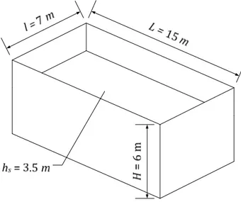
In order to validate the analytical developments briefly exposed in section 3, we can compare the corresponding results to those obtained by resorting to finite elements methods. As practical example, let us consider the reservoir depicted on Figure 3. It is characterized by a width of 7 m, a length of 15 m and a height of 6 m. It is filled with water up to a level of 3.5 m. The thickness tp of the two flexible walls is equal to 10 cm.
Figure 3. Main dimensions of the reservoir.
The physical properties defining the fluid and the solid are listed in Table 1. For this study, the reservoir is assumed to be made of steel.
Table 1. Properties for the fluid and the solid domains. Solid domain
Young modulus E 210 GPa
Poisson coefficient ν 0.3
Mass density ρ 7890 kg/m³
Fluid domain
Bulk modulus Kf 2.25 GPa
Speed of sound cf 1500 m/s
The finite elements software NASTRAN is used to perform a modal analysis of the reservoir shown on Figure 3. The flexible walls are modeled by using isoparametric quadrilateral CQUAD shell elements with four grid points, while hexahedral CHEXA solid elements with eight grid points are used for the fluid. The mesh size has been progressively reduced until a sufficient convergence on the results was reached.
Working with NASTRAN allows us to know the modal properties of the wet flexible walls. These ones may be confronted to the results obtained by our simplified method. As a matter of comparison, let us start by considering the eigenfrequencies. The values found numerically and analytically are presented in Table 2 for the seventh first modes of vibration.
Table 2. Comparison of the eigenfrequencies Mode number Analytical solution (Hz) Numerical solution (Hz) Relative error (%) 1 5.44 5.43 0.22 2 12.51 12.36 1.12 3 18.27 18.27 0.01 4 26.52 26.12 1.53 5 32.79 32.37 1.28 6 39.44 39.44 0.01 7 48.37 47.21 2.49
From Table 2, we see that the maximal discrepancy between the results given by NASTRAN and the ones derived by the present simplified approach does not exceed 3%, which seems to be acceptable. Moreover, this quite good agreement was obtained by considering only five dry modes (i.e. M = 5) in equation (13).
Figure 4. Vertical and horizontal planes π1 and π2 used for comparing the mode shapes.
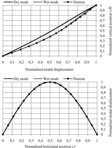
Let us now compare the wet mode shapes obtained for the flexible walls of the reservoir. The two first ones are plotted on Figure 5 and Figure 6 respectively. For each mode, two different illustrations are proposed. The upper one is a plot of the profile in the vertical plane z = l/2 (plane π1 on Figure 4), while the lower one corresponds to the profile in the horizontal plane y = H (plane on Figure 4).
Regarding the horizontal profile, it is clear that a sine half-wave seems to be a good approximation. Concerning the vertical one, the agreement appears to be satisfactory, even if some discrepancy may be observed near the top of the gate where water is not present.
Figure 5. Comparison of the first mode shape in π1 and π2
Figure 6. Comparison of the second mode shape in π1 and π2 0 0,1 0,2 0,3 0,4 0,5 0,6 0,7 0,8 0,9 1 0 0,1 0,2 0,3 0,4 0,5 0,6 0,7 0,8 0,9 1 N o rm al iz ed v er ti ca l p o si ti o n y /H
Normalized modal displacement Dry mode Wet mode Nastran
0 0,1 0,2 0,3 0,4 0,5 0,6 0,7 0,8 0,9 1 0 0,1 0,2 0,3 0,4 0,5 0,6 0,7 0,8 0,9 1 N o rm al iz ed m o d al d is p la ce m en t
Normalized horizontal position z/l Dry mode Wet mode Nastran
0 0,1 0,2 0,3 0,4 0,5 0,6 0,7 0,8 0,9 1 -1 -0,8 -0,6 -0,4 -0,2 0 0,2 0,4 0,6 0,8 1 N o rm al iz ed v er ti ca l p o si ti o n y /H
Normalized modal displacement Dry mode Wet mode Nastran
0 0,1 0,2 0,3 0,4 0,5 0,6 0,7 0,8 0,9 1 0 0,1 0,2 0,3 0,4 0,5 0,6 0,7 0,8 0,9 1 N o rm al iz ed m o d al d is p la ce m en t
Normalized horizontal position z/l Dry mode Wet mode Nastran
The comparisons illustrated here above for this reservoir show that the agreement between the analytical and numerical results is satisfactory. This tends to validate the theoretical derivation of the vibration properties for an immerged plate by using the Rayleigh-Ritz method. The present analytical approach has also been corroborated by additional comparisons performed with other various reservoirs that are not presented here.
5 DYNAMIC ANALYSIS OF A WET PLATE 5.1 Equilibrium equation
The modal analysis of immerged flexible walls performed in the previous section provides a global insight on the way such structures respond to a seismic excitation. The next step is now to consider the situation where the reservoir is submitted to an earthquake load having a longitudinal acceleration component denoted by Ẍ(t).
To get an analytical approximation of the dynamic response of the reservoir in such circumstances, we can refer to the equilibrium equation (1). Nevertheless, this one will be modified here to account for an eventual damping that may affect the structure. If we denote by fd the damping forces, equation (1) becomes:
(
X u)
f D u ptp &&+&& + d + ∇4 =−
ρ
(19)In order to characterize a bit further the term fd, we will assume that these additional forces are directly related to the velocity. Assuming a Rayleigh-type damping, fd may be seen as having two different contributions: a first one coming from the mass of the structure and a second one coming from its stiffness. According to Shames [8], we can write:
u D u t
fd =
αρ
p&+β
∇4& (20) where α and β are two constants known as the Rayleigh damping coefficients. Furthermore, if we rearrange (19), we get:(
)
(
p t X u t u D u)
u
D∇4 =− −
ρ
p &&+&& −αρ
p&+β
∇4& (21) which may be identified as the equilibrium equation of a plate submitted to an external resulting horizontal action fext given by the right hand side of (21). In fact, fext is nothing more than the sum of the pressure, damping and inertial forces. On the contrary, the left hand side of (21) may be seen as an internal force fint.5.2 Virtual work principle
Once all the forces acting on the structure have been characterized, we can try to derive analytically the forced vibrations of an immerged plate. To do so, a solution is to apply the virtual work principle, which simply states that a necessary and sufficient condition for equilibrium is to equate the external and internal virtual works for any kinematically compatible displacements field. Consequently, if we want to express the equilibrium of the plate, we first may consider a compatible virtual field δu(y,z,t) acting on it.
Furthermore, if we consider the developments performed in section 3.3, it seems reasonable to express that the motions
u(y,z,t) exhibited during the seismic excitation are based on the wet mode shapes. In other words, we postulate that:
( ) ( )
∑
( ) ( )
∑
= = ∆ = ∆ = N k k k N j j j t y z u q t y z q u 1 1 , ,δ
δ
(22)where N is the number of wet modes used for developing u(y,z,t). At this stage, the modal amplitudes qj and δqk are still unknown but will be determined by applying the virtual work principle.
5.3 Internal virtual work
During the virtual displacement δu, the work performed by the internal forces fint is simply given by:
∫∫
∫∫
⋅ ⋅ = ∇ ⋅ ⋅ = H l H l dydz u u D dydz u f W 0 0 4 0 0 int intδ
δ
δ
(23)which may be transformed by considering the modal decomposition (21). Doing so leads to an expression of δWint involving the wet modes calculated in section 3.3:
∑ ∑
= = = N k N j jk j k qU q W 1 1 intδ
δ
(24)5.4 External virtual work
If we now develop the second part of the virtual work theorem, the work associated to the external forces during the virtual displacement ( , , ) is given by:
∫∫
⋅ ⋅ = H l ext ext f u dydz W 0 0δ
δ
(25)and subsequently, we have to examine the contributions coming from all the terms involved in the right hand side of (21). This task is quite fastidious, so we will only provide here a short summary of the final results, obtained after having incorporated the modal form (21) into (25). The following results can be easily proved (see also in the Appendix for more details):
• For the inertia forces, we get the following virtual work:
∑
∑
∫∫
= = ∆ + − N k H l k p N j jk j k q T X t dydz q 1 1 0 0ρ
δ
&& && (26)• For the Rayleigh damping forces, we get the following virtual work:
(
)
∑ ∑
= = + − N k N j jk jk j k q T U q 1 1β
α
δ
& (27)• For the pressure, we get the following virtual work:
∑
∫∫
∑
= = − ∆ − N k N j jk j H l k r k p dydz q W q 1 0 0 1 & &δ
(28)5.5 Global equilibrium equation
If we gather all the results obtained in (24), (26), (27) and (28), we can write the virtual work principle in the following way:
(
)
(
)
X V U q U T q W T q k N j jk j N j jk jk j N j jk jk j & & & & & = + + + −∑
∑
∑
= = =1 1 1β
α
(29)with k = 1,2, ... , N. It is worth noting that the virtual coefficients δqk do not appear anymore in (29) as the virtual work principle has to be satisfied for any value of these parameters. Furthermore, it is important to recall that Tjk, Ujk, Wjk and Vk may be directly expressed with help of the wet mode shapes. Some more detailed results are given in the Appendix.
As a final step, let us write (29) under a matrix form. If we introduce the matrices [T], [U], [W] and the vectors q and V, we can express (29) by the following more classical result:
[ ] [ ]
(
T −W)
q&&(t)+(
α
[ ] [ ]
T +β
U)
q&(t)+[ ]
U q(t)=V&X&&(t) (30) For a given acceleration Ẍ(t), this equation may be solved by using the classical Newmark integration scheme for example. Doing so leads to the vector q containing the coefficients qj. These ones are then used to derive the dynamic response of the flexible walls with help of equation (22).6 NUMERICAL EVALUATION OF THE DYNAMIC
RESPONSE
6.1 Description of the seismic action
To validate the analytical developments briefly exposed in section 5, we can compare them to those obtained by using a finite element model. The reservoir considered in section 4 (Figure 3), for which the material and fluid properties are those listed in Table 1, is submitted to a seism having the longitudinal acceleration Ẍ(t) depicted on Figure 7.
Figure 7. Longitudinal component of the seismic acceleration The Fourier transform of this signal, represented on Figure 8, shows that the main part of the seismic excitation is located in the frequency range [1 Hz ; 15 Hz].
Figure 8. Fourier transform of the seismic acceleration 6.2 Description of the model
The numerical analysis is performed by using the finite elements software LS-DYNA. The flexible walls are modeled with Belytschko-Tsay shell elements [10] of uniform thickness tp. The constitutive material is supposed to be elastic and characterized by a mass density ρ, a Young modulus E and a Poisson ratio ν (see Table 1). The stress and strain tensors are related according to the classical Hooke's law.
The mesh of the solid domain is quite coarse, with a more or less regular size of 20 × 20 cm for the shell elements. This choice is due to the necessity of limiting the size of the model. Nevertheless, we also performed simulations on more refined models with a meshing of 5 × 5 cm or 10 × 10 cm, and the obtained results were not sensitively different from the present ones.
The fluid is modeled with constant stress solid elements [10] and supposed to behave like an elastic medium characterized by a mass density ρf and a bulk modulus Kf (see Table 1), but without shearing forces inside this material. This is coherent with the behavior of water.
The mesh of the fluid domain is also regular, with an approximate size of 19 cm for the solid elements. Here again, using more refined meshes does not change noticeably the results.
The both previous meshes representing the water and the structure do not share any node in common, which means that the fluid nodes are allowed to slide on the solid walls. A penalty contact algorithm is used to simulate the interaction between the plate and the surrounding liquid, which prevents the fluid from passing through the structure.
6.3 Presentation of the results
The analytical predictions derived from the virtual work principle are now confronted to the numerical ones. In this section, we will limit our presentation to the case of the reservoir depicted on Figure 3. Structural damping is applied on LS-DYNA through the classical Rayleigh formulation. The mass and stiffness coefficient are calibrated so as to model an arbitrary 4 % damping on the two first modes of vibration.
It is worth mentioning that many other additional simulations were performed, using different geometrical configurations than the one of Figure 4. The conclusions that we found in all cases are very similar to those presented here, so for conciseness, we will not present them in this paper. -1 -0,8 -0,6 -0,4 -0,2 0 0,2 0,4 0,6 0,8 1 0 1 2 3 4 5 6 7 8 9 10 11 12 13 14 15 A cc el er at io n ( m /s ²) Time (s) 0 0,02 0,04 0,06 0,08 0,1 0,12 0 5 10 15 20 25 30 35 40 M ag n it u d e (m /s ²) Frequency (Hz)
Figure 9. Comparison over four different time intervals
As matter of comparison between analytical and numerical results, we can compare the total hydrodynamic force F(t) applied on the flexible wall (in excess to the hydrostatic pressure) is plotted on Figure 9 for different time intervals. As we neglect here the convective contribution, this resultant force is simply obtained by integrating the rigid and flexible impulsive pressures pr and pf over the wall surface.
We see that the agreement between analytical results and numerical ones is quite satisfactory. The comparison of the extreme values, extracted from the previous curves and listed in Table 3, shows that the theoretical model tends to be more conservative than the finite element one. Moreover, the maximal overestimation does not exceed 15 %, which is acceptable for a pre-design study. Analytical and numerical simulations performed for other reservoirs led to similar conclusions.
Table 3. Comparison of the extreme values Result Analytical solution (kN) Numerical solution (kN) Relative error (%) Maximal value 180.09 kN 157.36 kN 14.4 Minimal value -179.88 kN -167.29 kN 7.5 7 CONCLUSION
In this paper, we briefly present an analytical procedure to analyze the dynamic response of flexible reservoirs submitted to an earthquake.
To achieve this goal, we first evaluate the wet modes characterizing the free vibrations of a plate in contact with water on one side. These modal properties are derived by using the Rayleigh-Ritz method. To check the validity of the results given by this approach, we compare them to numerical solutions obtained by using the finite elements software NASTRAN. These ones are derived by performing a modal analysis on a model where both the fluid and the solid are represented. For all the reservoirs tested, the agreement with the analytical results is found to be satisfactory.
As soon as the wet modal properties are derived, it is possible to have a better investigation of the dynamic response of a reservoir submitted to a seism. The virtual work principle is used to derive an analytical solution to the problem. This one is then validated by comparison with numerical results provided by the software LS-DYNA. Once again, a sufficient agreement is found between analytical and numercial results.
In comparison with numerical techniques, the main advantages of the present approach may be summarized in the following way:
• The method quickly provides the approximate time evolution of the total hydrodynamic pressure acting on a flexible wall for a given acceleration Ẍ(t). This may be particularly useful during the early design stages of new structures, when engineers do not necessarily have time to resort to finite elements software.
• In comparison with numerical approaches, our simplified method has also the advantage of being quite intuitive. Indeed, using finite elements software is still quite arduous, as having a proper numerical representation of -200 -150 -100 -50 0 50 100 150 200 0 0,3 0,6 0,9 1,2 1,5 1,8 2,1 2,4 2,7 R es u lt in g f o rc e (k N ) t (s) LS-DYNA Analytical -200 -150 -100 -50 0 50 100 150 200 2,7 3 3,3 3,6 3,9 4,2 4,5 4,8 5,1 5,4 R es u lt in g f o rc e (k N ) t (s) LS-DYNA Analytical -200 -150 -100 -50 0 50 100 150 200 5,4 5,7 6 6,3 6,6 6,9 7,2 7,5 7,8 8,1 R es u lt in g f o rc e (k N ) t (s) LS-DYNA Analytical -150 -100 -50 0 50 100 150 8,1 8,4 8,7 9 9,3 9,6 9,9 10,2 10,5 10,8 R es u lt in g f o rc e (k N ) t (s) LS-DYNA Analytical
the fluid-structure interaction is not that easy. This requires from engineers to be highly familiar with all the various modeling techniques, which is not necessarily always the case.
• Finally, we can also argue that the present simplified method is particularly well suited for working with important structures (such as lock chambers or large reservoirs). Indeed, such configurations may lead to very huge finite elements models requiring non negligible calculation times.
Even if this paper is only dealing with the seismic design of reservoirs, it constitutes a first step for developing a similar simplified tool applicable to lock gates. Indeed, the main difference between the reservoir considered here and a lock chamber is that the flexible walls have to be replaced by the lock gates. By following a similar analytical procedure, it should be therefore possible to derive the same kind of results for these particular structures. This will be precisely the goal of further investigations.
APPENDIX
This appendix provides a more detailed description of the formulae leading to the evaluation of the matrices [T], [U], and [W] introduced in equation (30). These matrices are only functions of the wet eigenmodes of vibration. These last ones are given by (13) and may be derived by following the procedure described in section 3. As soon as they are found, they can be introduced in the following expressions:
( )
(
)
(
)
( ) 1 0 ) ( 0 0 4 0 0 sinh cosh 1 2 mnk n m j mn mn m s mn mn f jk H l k j jk H l k j p jk I I L l h L W dydz D U dydz t T∑∑
∫∫
∫∫
∞ + = ∞ + = − = ∆ ∆ ∇ = ∆ ∆ =ξ
ξ
ξ
ρ
ρ
(31)where Imn has already been defined by equation (12). In addition, the various components of the vector V are to be found by applying the subsequent relation:
( )
(
)
∫∫
∫∫ ∑
∆ − ∆ ⋅ − = +∞ = H l k p k h l n n s n n f k dydz t dydz L h y L V s 0 0 0 0 1 2 cosh 2 cosh 4ρ
β
β
β
ρ
(32)where βn = (2n − 1)π/L and ρf is the mass density of the fluid, as mentioned previously.
REFERENCES
[1] H.I. Epstein, Seismic design of liquid storage tanks, Journal of the Structural Division, Vol. 102, No 9, pp.1659-1673, 1976.
[2] M.A. Haroun, Stress analysis of rectangular walls under seismically
induced hydrodynamic loads, Bulletin of Seismological Society of
America, Vol. 74, No. 3, pp. 1031-1041, 1984.
[3] G.W. Housner, Dynamic pressures on accelerated fluid containers, Bulletin of Seismological Society of America, Vol. 47, No. 1, pp. 15-37, 1957.
[4] R.A. Ibrahim, Liquid sloshing dynamics: theory and applications, Cambridge University Press, Cambridge, United Kingdom, 2005. [5] A.W. Leissa, The free vibration of rectangular plates, Journal of Sound
and Vibration, Vol. 31, No. 3, pp. 257-293, 1973.
[6] J.K. Kim, H.M. Koh, I.J. Kwahk, Dynamic response of rectangular
flexible fluid containers, Journal of Engineering Mechanics, Vol. 122,
No. 9, pp. 807-817, 1996.
[7] C. Rajalingham, R.B. Bhat, G.D. Xistris, Vibration of rectangular plates
using plate characteristic functions as shape functions in the Rayleigh-Ritz method, Journal of Sound and Vibration, Vol. 193, No. 2, pp.
497-509, 1996.
[8] I.H. Shames, C.L. Dym, Energy and finite element methods in structural
mechanics, New Age International Publishers, New Dehli, India, 1995.
[9] MSC Software, MSC NASTRAN reference manual, MSC Software
Corporation, Santa Ana, United States, 2012.
[10] J.O. Hallquist, LS-DYNA theoretical manual, Livermore Software