Broadcast Strategies and Performance Evaluation of IEEE 802.15.4 in Wireless Body Area Networks WBAN

(1)

HAL Id: hal-01404848

https://hal.archives-ouvertes.fr/hal-01404848v2

Submitted on 6 Jun 2019

HAL is a multi-disciplinary open access

archive for the deposit and dissemination of

sci-entific research documents, whether they are

pub-lished or not. The documents may come from

teaching and research institutions in France or

abroad, or from public or private research centers.

L’archive ouverte pluridisciplinaire HAL, est

destinée au dépôt et à la diffusion de documents

scientifiques de niveau recherche, publiés ou non,

émanant des établissements d’enseignement et de

recherche français ou étrangers, des laboratoires

publics ou privés.

Broadcast Strategies and Performance Evaluation of

IEEE 802.15.4 in Wireless Body Area Networks WBAN

Wafa Badreddine, Claude Chaudet, Federico Petruzzi, Maria Potop-Butucaru

To cite this version:

Wafa Badreddine, Claude Chaudet, Federico Petruzzi, Maria Potop-Butucaru. Broadcast Strategies

and Performance Evaluation of IEEE 802.15.4 in Wireless Body Area Networks WBAN. [Research

Report] LIP6 UMR 7606, UPMC Sorbonne Universités, France; UPMC - Paris 6 Sorbonne Universités.

2016. �hal-01404848v2�

(2)

1

Broadcast Strategies and Performance Evaluation of IEEE

802.15.4 in Wireless Body Area Networks WBAN

Wafa Badreddinea,∗_{, Claude Chaudet}b_{, Federico Petruzzi}a_{, Maria Potop-Butucaru}a

a_{Sorbonne Université, LIP6-CNRS UMR 7606, Paris, France}

b_{Webster University Geneva, Bellevue, Switzerland}

Abstract

Wireless Body Area Networks (WBANs) can be considered as an evolution of wireless sensor networks towards wearable and implanted technologies. Radio propagation and mobility are particular in this context, as they are influenced by the characteristics and movement of the human body and by the necessity to keep the transmission power at its minimum to save energy and limit interactions with the wearer.

In this paper, we investigate the broadcasting problem in which a node, typically the gateway, tries to send a packet to all other nodes in the network at minimal cost. This problem is not triv-ial and we show through simulation that forwarding strategies coming from the Delay Tolerant Networks world cannot be transposed without adaptation. We enriched the Omnet++ simulator with a WBAN-specific channel model issued from recent research on biomedical and health in-formatics and use this model to evaluate 9 classes of broadcasting algorithms, including our own proposals, with respect to their ability to cover the whole network, their completion delay, their cost in terms of transmissions and their capability to preserve multiple packets order (i.e. total order broadcast).

Our study shows that there is a subtle compromise to find between verbose strategies that achieve good performance at the cost of numerous transmissions, ultimately provoking collisions and more cautious solutions that miss transmission opportunities because of mobility.

Keywords: Body Area Networks, Broadcast, Mobility, Forwarding

1. Introduction

Wireless Body Area Networks (WBANs) open a new area within Wireless Sensor Networks (WSN) research, in which on-body and invasive sensors collaborate and communicate to monitor, collect, process and transmit measurements of various body parameters. Movements can be tracked and predicted to help capturing motion with applications in virtual reality, gaming, sports

∗_{Corresponding author}

Email addresses: wafa.badreddine@lip6.fr (Wafa Badreddine), chaudet@webster.ch (Claude Chaudet), petruzzi.frederico@lip6.fr (Federico Petruzzi), maria.potop-butucaru@lip6.fr (Maria Potop-Butucaru)

(3)

as well as in detecting falls and accidents. Monitoring physiological signs such as blood pressure, heart rate, body temperature or blood composition has some great potential in healthcare.

There is a consensus that devices collaboration fosters optimization. At the application level, additional measurements can be triggered automatically when a parameter crosses a threshold for example. At the network level, multihop communication allows to reduce transmission power and control energy expenditure and devices temperature and improves spatial reuse. In this sense, WBANs are no different from traditional sensor networks. Yet they differ in many other aspects: the size of the network is limited to a dozen of nodes, and scalability is not an issue. Transmis-sion power is usually kept as low as possible, not only to reduce interferences and to improve devices autonomy and lifetime, but also to reduce wearers exposure to electromagnetic signals and consequences from devices temperature. One should note that autonomy may be a critical factor to optimize when sensors are implanted. This results in creating short-range wireless links with a variable quality depending on the wearer’s posture as much as on the environment. Body absorption, reflections and interference cannot be neglected, and maintaining a direct one-hop link between a central node and all peripheral nodes is probably not the most effective strategy. However, in a multi-hop scenario, communication protocols would greatly benefit from taking into account the particular in-network mobility that results from the body movements.

Indeed, if devices were aware of the mobility pattern characteristics, they could use this information to predict the best packets scheduling and optimize bandwidth usage and energy, as well as to limit radio emissions. Delay-tolerant networks have been the first type of net-works to consider explicitly and to actually use network mobility to improve packets forwarding. They address the intermittency of communication links by using a store-and-forward philosophy. However, most of the DTN communication protocols were designed either to address mobility schemes with long disconnection periods, or fully stochastic mobility patterns like random walks. WBANs exhibit an almost periodical mobility with fast and comparable links on and off periods. In this paper, we focus on the broadcasting problem from a source to all destinations. Broad-casting is not the primary traffic pattern in these networks, but it is fundamental for network-level operation like maintenance of the routing tree, as well as at the application level, for reconfig-uration or for transmitting emergency messages. We analyze the behavior of various broadcast strategies adapted from DTN literature and propose an alternative strategy from the analysis of the strengths and weaknesses of the different approaches. We compare network coverage, com-pletion delay and required transmissions of 9 different algorithms over human body mobility traces.

The paper is organized as follows: Section 2 presents the context and the broadcast problem. Section 2.2 introduces relevant related works and presents various broadcast strategies, including an original contribution, that we have compared through simulation in Section 4. Section 4 first describes the limitations of the standard channel models proposed by OMNET++, then describes the realistic channel model we implemented and finally presents and compares different broadcast strategies with respect to success probability, latency, traffic volume and energy.

2. Context

2.1. Routing in multi-hop networks

Mobility in Body Area Networks has some specific characteristics that makes these network different from other categories of wireless multi-hop networks. Wireless links are not stable and may appear and disappear according to a pattern that depends on the location of the nodes and on

(4)

the posture of the wearer. Naganawa et al. (in [1]) modeled a 2.45 GHz WBAN channel over 7 links between on-body nodes equipped with 5mm dipole antennas. They considered 7 movement postures initially modeled in [2] using Poser and determined the channel characteristics using the Finite-Difference Time-Domain method [3].

20 30 40 50 60 70 80 0.0 0.1 0.2 0.3 0.4 0.5 Path loss (dB) Density

Upper arm − Ankle ; Running Upper arm − Ankle ; Sleeping Upper arm − Head ; Sleeping Upper arm − Head ; Lying down

Figure 1: PDF of the path loss between upper arm node and other nodes in different positions (Data source [1])

Figure 1 illustrates the variability in links characteristics by showing the density function of the path loss for two of these links in different positions. Nodes would rather use links that are strong, i.e. exhibit a low average path loss, and reliable, i.e. have a low variance. However, a position change may increase the variance significantly and there is no guarantee that the network may remain connected with only low variance links.

A high variation usually reflects movements that may be quasi-regular, resulting in frequent but predictable link connections and disconnections. Classical routing protocols may choose to use or not such links, but to the best of our knowledge, none of the proposed routing proto-cols in ad-hoc, sensor or delay-tolerant networks was designed to address specifically links with comparable on and off periods and possible sudden changes.

Ad-hoc proactive and reactive protocols both seek to select links and establish paths for at least the duration of a communication. Oscillating links, as found in WBANs, may result in a random selection of the links composing paths, depending on the moment when control messages are emitted. The instability will then provoke several retransmissions.

Wireless Sensor Networks (WSNs) protocols may be more adapted to links intermittence, nodes turning their radio on and off regularly to save energy. However, most sensor networks routing protocols either assume that these duty cycles are homogeneous across the network, or that they can be influenced to help routing. In WBANs, the disconnections periods are defined by nodes relative mobility, which is neither perfectly regular, nor identical between each couple of nodes. Besides, in sensor networks, each node decides of its own duty cycle and could announce it to its neighbors, the only remaining variation then resulting from the clock skew between nodes.

(5)

WBANs could therefore be closer to some types of delay tolerant networks (DTN) which are designed to handle connections and disconnection periods. Links intermittent behavior is assumed and handled by having nodes work in store-and-forward mode, buffering packets until a desired link appears. Several papers such as [4, 5] propose and evaluate mobility-aware shortest path algorithms in DTNs. Even though they address unicast routing, these contributions confirm that efficiency increases with the knowledge of the mobility pattern. In other words, knowing how nodes move allows to reduce the number of unnecessary transmissions and the delivery delay.

In Interplanetary networks (IPN) that connect satellites orbiting around planets, the orbiting objects have predetermined paths and it is possible to predict connections and disconnection with a good accuracy. Routing protocols in IPNs use this regularity to schedule transmissions. In WBANs, the mobility pattern may be quasi-periodical, but some degree of uncertainty exists and links disappear quickly in case of fast motion, which makes it difficult to make predictions. Besides, the wireless channel is less reliable in WBAN than in space.

In vehicular applications of delay tolerant networks, buses or cars exchange data whenever they meet. Even if the inter-connection delays and the connectivity periods are less regular than in IPN, most solutions consider that connection periods are much shorter than inter-connection intervals, which results in a relatively short transmission window that needs to be detected and used at its best.

In WBANs, the on and off periods are usually comparable for each link. In most scenarios, except static ones, movements are relatively regular and connections and disconnection periods are of comparable lengths. Even if we can take inspiration from DTN and their store-and-forward philosophy, there is no strong need to influence packets scheduling to make the most of infrequent and short relevant transmission opportunities.

2.2. Broadcasting in multi-hop networks

Broadcasting algorithms for multi-hop networks can be classified into two major categories: dissemination(or flooding) algorithms require no particular knowledge of the network versus Knowledge-basedalgorithms, which use some information of the network mobility to predict spatio-temporal connectivity and to reduce the number of transmissions. Dissemination algo-rithms tends to generate multiple copies of the same message, which explore all paths in parallel and improve mechanically the delivery probability while reducing the delay until congestion ap-pears. Such strategies generate a large number of unnecessary transmissions and are not energy-efficient. Understanding and using the nodes mobility pattern leads to a better efficiency, but acquiring the necessary information has a cost and there is a subtle balance to find between duplicate data packets and control messages.

In their seminal paper [6], Ni et al. name and analyze the broadcast storm problem that happens in mobile ad-hoc networks: blind flooding generates numerous transmissions all over the network, causing collisions, increasing contention and redundant transmissions. To alleviate this effect, each node can simply condition its retransmission to a constant probability, or take a forwarding decision based on the number of copies received during a certain time frame, on the distance between the source and the destination or on the location of the nodes if it is available. They also examine the effect of partitioning the network in 1-hops clusters, the cluster heads forming a dominating set among the network. The dominating sets-based approaches will be the source of numerous contributions, but is not really relevant in WBANs, as the size and diameter of the network remains very limited.

(6)

Many works have explored the probabilistic flooding approach, also called Gossipping. Haas et al.[7] identify the existence of a threshold on the forwarding probability below which gossip-ing fails to deliver the message. Sasson et al., in [8] use percolation theory to characterize this phase transition threshold on random graphs. Neither of these works are directly applicable to WBANs, as the mobility pattern is very different and non-homogeneous, but they both show that the networks shape and dynamics have an influence on the optimal forwarding probability.

Vahdat et al., in [9] were among the first to consider that end-to-end connectivity was not guaranteed permanently. They rather consider a network formed of different connected groups of nodes that eventually meet. They introduce epidemic routing, whose first step consists in dissem-inating information inside a group through basic flooding. When two nodes meet, they exchange a summary vector containing the messages ID they already possessÂ and then exchange only the missing messages that will propagate through new clusters this way.

In [10], the authors compared various strategies for controlling flooding in delay tolerant networks, assuming that nodes have no knowledge about their location or their mobility. They compare performance of probabilistic approaches with different approaches limiting flooding impact using a time to live, expressed either in number of hops, or as an expiration date. Unsur-prisingly they show that these strategies can effectively reduce the load induced by flooding the network without increasing significantly the completion delay, or the failure probability.

Spray and Wait, [11], is an original routing strategy that decomposes the transmission process in two phases. In the spray phase, multiple copies of the message are sent in the network with a flooding-like mechanism. Then the nodes who hold copies of the message start waiting until they meet the destination to which they will transmit the message directly. Spray and Focus [12] goes one step beyond by letting nodes that hold one of the message copies forward it using an utility function, rather than waiting to meet the destination. These strategies are not flooding strategies, however they show how controlling and limiting the number of copies of the same message that travel in the network affects the delivery performance.

In the k-neighbor broadcast scheme [13], a packet is retransmitted if and only if the number of neighbors present exceed a threshold, K, and if at least one of these neighbors did not receive the message yet. Even if the implementation is different, we find back here the concepts behind epidemic routing and the notion of not systematically transmitting a packet to reduce the number of transmission.

Concerning WBANs, several routing protocols have been proposed in the past decade [14, 15, 16]. Most protocols are adaptations of classical strategies to the WBAN context. A series of protocols aim at reducing the heat generated by devices to avoid interaction with the biologic pro-cesses [17, 18, 19, 20, 21]. Quwaider and Biswas [22] propose an opportunistic routing scheme able to switch between direct links and multihop paths when getting out of line of sight. In [23], authors propose ESR that is based on on-demand routing scheme. A path routing selection is processed based on two functions: energy cost function and path stability function. Even if au-thors assume mobility they did choose a simple mobility model: the Random Waypoint model. In addition, path discovery process generates a lot of traffic that can not be neglected.

DTN like solutions [24] and many other WBAN proposals (such as EDSR [25] or Co-CEStat [26]) do not take into account the mobility of the human-body: during the transmissions of the message over the path already computed, disconnections can happen causing failures. Liang et al.[27] let the nodes sample link qualities over a few time slots to predict the best moments to transmit. [28] uses a similar approach to update a vector of likelihoods that a link will be available in a given time slot. They show through simulation and experiments that taking into account the particular mobility of the body improves transmission delay when compared to a

(7)

traditional probabilistic algorithm for DTN.

3. Comparing Broadcast Strategies

As forwarding/routing in multi-hop networks has been very active in the past decades, several strategies are available when it comes to broadcasting. However, there is no definitive answer with respect to the specificities of the WBAN context yet. Our goal, in this work is to compare the classical strategies categories to shed light on their strengths and weaknesses.

We consider that the Gateway node initiates the communication at the application layer, which is then sent throughout the network. When a node receives a broadcasted packet, it needs to take a decision whether to transmit it to the application layer, to forward it and to which of its neighbors and when, or to discard it. It bases its decision on the broadcasting algorithms and on the packet characteristics. Nodes may examine the packet’s time to live (TTL) to evaluate how long it has been in the network, or its sequence number, which can give an indication on whether the packet has already been received or not.

Here, we are interested in network related aspects only and make abstraction of the system aspects such as the memory required to store all received sequence numbers. Practical solutions to these issues exist and may be appropriate or not depending on the scenario. For example, storing only the last sequence number per source is valid when dealing with successive updates that supersede each other. TCP-like solutions are also possible when all messages need to be received.

As the literature suggests, understanding the nodes relative mobility can improve the for-warding decision, but capturing nodes mobility has a cost. It either requires a precise nodes localization mechanism, which is typically achieved by measuring round-trip time of flights between couple of nodes in IR-UWB networks, or relies on hello messages to learn connec-tion/disconnection patterns. In both cases the gain acquired by optimizing the broadcast process can quickly be lost to control traffic.

In the rest of this article, we compare the performance of the following categories of strate-gies:

Flooding designates the simplest strategy: nodes forward each received packet as long as the packet’s TTL is greater than 1 and decrement this value in the packet by 1 upon transmis-sion.

Plain Flooding is more restrictive: using sequence number, a received packet is delivered to the application layer and forwarded if and only if it has never been received before. Redundant copies are discarded and each node emits each packet at most once.

Probabilistic Flooding (P=0.5) : nodes broadcast packets according to a constant probability, P. The choice of the correct value for this threshold depends on the scenario, which makes this type of solution difficult to adapt in practice. For our evaluation scenarios, we realized simulations for various values of the P parameter that show the same trend: the lower the probability, the worse the network coverage is. In this paper, we chose to present results for a probability P= 0.5 to show the compromise between a very cautious strategy failing to cover the network (e.g. P= 0.3) and flooding (P = 1)1.

1_{Results for di}_{fferent P values are available online: http://www.chaudet.ch/WBAN/}

(8)

Probabilistic flooding (P=P/2) : nodes decide to broadcast each packet according to a proba-bility P that is divided by 2 every time the same packet is re-broadcasted. The probaproba-bility depends on each node and is not embedded in the packets; nodes maintain a local table of packets identification and associated probabilities. In our simulations, the initial forward-ing probability is set to 1.

Pruned Flooding (K) : each node forwards each packet only to K neighbors, chosen randomly per packet according to an uniform distribution. The choice of the parameter, K has a strong influence on the protocol performance, as confirmed by our simulations. This strat-egy requires a node to identify its neighbors and hence induces control traffic. It also transforms the broadcasting process into multiple unicast transmissions, but can, in prac-tice, be implemented over a broadcast medium by embedding the designated neighbors list in each packet’s header.

Tabu Flooding : each packet contains the list of nodes it has been forwarded by. This infor-mation is, of course, different for different instances of the same packet and issues related to the maximum packet size can be ignored given WBAN’s classical diameter. Each node uses this information to forward packets only to yet uncovered nodes, which requires nodes to identify their neighbors and, as in Pruned Flooding, may transform the broadcasting process into multiple unicast transmissions.

EBP (Efficient Broadcast Protocol) (I; K) [13]: nodes only broadcast a packet when they are surrounded by at least K neighbors, and if at least one of these neighbors has not received the packet yet. Nodes exchange every I seconds Hello packets containing their identifica-tion and the list of packets they already received, which can be limited to the last sequence number received depending on the application. Nodes could also identify packets received by their neighbors through overhearing.

In the original EBP, the threshold value, K, was considered constant and uniform across the network. In a WBAN environment, adapting this value to the location of nodes in the network seems natural, as some nodes are more natural forwarders than others. In the implementation we evaluate in this paper, K is set to 2 for the Gateway node (chest), to 2 for the head and ankle (peripheral nodes) and to 1 for the other nodes (center nodes). Two Hellofrequencies are considered: every I= 0.25 s and I = 0.5 s.

MBP: Mixed Broadcast Protocol (NH; Q; T ) : we proposed this strategy in [29] as a mix between the dissemination-based and knowledge-based approaches. The broadcast begins as a basic flooding algorithm (i.e Flooding strategy). When a node receives a message, it checks the number of hops δ this message has traveled since its emission by the Gateway, either embedded in packets as an explicit value, or using the TTL, and compares it to a threshold, NH:

• As long as δ < NH, node forwards the packet, using simple flooding, broadcasting the packet to all neighbors in range.

• When δ ≥ NH, node waits during a time T to receive up to Q acknowledgments sent by neighbors (see below).

– if it receives a number of acknowledgments greater or equal than Q, the node stops rebroadcasting the message.

(9)

– if it fails to receive Q acknowledgments within T , it broadcasts the packet. • When δ > NH nodes sends, in addition, an acknowledgment to the node it received

the packet from. Note that in a real implementation, these acknowledgments could be implicit when nodes decide to rebroadcast the packet.

This algorithm depends on three main parameters to continue or stop the broadcast: NH, the threshold on the number of hops traveled so far, Q, the number of expected acknowl-edgments and T the timeout that triggers the next forwarding attempt. All parameters have an influence on the algorithm performance that we evaluated through simulation. Con-cerning Q, we determined that the best performance was achieved with different values according to node position: for example, for non natural forwarder nodes like head and ankle nodes, Q should be set to 0. In our simulations we set Q= 0 for the head and ankle nodes, Q= 2 for the chest node and Q = 1 for all the other nodes. The timeout has been set to T = 0.2 s. In section 4, we show results for NH equals to 1, 2 and 32_.

Optimized Flooding in addition to the aforementioned protocols, we introduce here for com-parison a new protocol named Optimized Flooding. This protocol aims at achieving a better compromise between traffic and performance by limiting packets retransmissions with two counters:

• cptGlobal is embedded into each copy of the packet itself. Every time the packet is received by a node that had not received it previously, cptGlobal is increased before forwarding to reflect the fact that the packet reached a new node.

• CptLocal is a per-packet variable local to each node. It is a local copy of the maxi-mum value of cptGlobal that the node has seen so far.

The general idea of this algorithm is to limit packets transmissions with respect to flood-ing without any additional control traffic, e.g. to identify neighbors. The two counters (cptGlobal and C ptLocal) act as indicators of the behavior of the packet and are used to avoid packets traveling a too long and redundant road (cptGlobal) and to avoid ping-pong effects between close nodes (CptLocal).

Optimized Floodinglimits broadcasting by comparing packets cptGlobal values with local C ptLocalvalues. When cptGlobal is lower than C ptLocal, the packet instance received has traveled a shorter path than a previous instance and is redundant. Both counters are limited by a maximum value, cptMax, which limits packets journeys. In a conservative approach cptMax is set by default to the number of nodes in the network. Upon reception of a broadcasted packet, each node applies algorithm 1. This algorithm does not need information on the neighbors and hence relies only on data packets. It however requires to keep track of the nodes that forwarded instances of the packets, and may require storing list of forwarders in each packet header.

4. Performance Analysis of Broadcast Strategies

We implemented the algorithms described in Section 3 in a WBAN scenario in the Omnet++ simulator. Omnet++ provides a set of modules that specifically model the lower network layers

2_{Additional results are available online: http://www.chaudet.ch/WBAN/}

(10)

Algorithm 1 Optimized Flooding algorithm: take a forwarding decision when receiving a packet

1: procedure Upon reception(m<S eqNum, T T L, C ptGlobal>)

2: if Upon receiving for the first time then . based on S eqNum

3: cptGlobal ← cptGlobal+ 1

4: cptLocal ← cptGlobal

5: Deliver(m)

6: if T T L>1 then

7: Broadcast(m<S eqNum, TT L, CptGlobal>)

8: end if

9: else

10: if cptGlobal never increased by this node for this copy of the message m then

11: cptGlobal ← cptGlobal+ 1

12: end if

13: if cptGlobal= cptMax then . cptMax = Number of nodes in the network

14: Discard m . All nodes have received the packet

15: else

16: if cptGlobal ≤ cptLocal then . a better instance has been received before

17: Discard m

18: else

19: if T T L>1 then

20: cptLocal ← cptGlobal

21: Broadcast(m<S eqNum, CptGlobal>)

22: else 23: Discard m 24: end if 25: end if 26: end if 27: end if 28: end procedure

of WSN and WBAN, thanks to the Mixim project [30]. It includes a set of propagation models, electronics models and power consumption models, as well as diverse medium access control protocols.

4.1. WBAN Specific Channel Model

The MoBAN framework for Omnet++ adds mobility models for WBANs composed of 12 nodes in 4 different postures. Unfortunately the MoBAN code mainly focuses on the mobility re-sulting from the change of position, rather than describing coherent and continuous movements. Besides, it models the movement of each node with respect to the centroid of the body and the signal attenuation between couples of nodes is approximated with a simple propagation formula that is not accurate enough to model low-power on-body transmission. It neither models ab-sorption and reflection effects due to the body, nor alterations due to the presence of clothes or interference from other technologies at the same frequency since 2.4 GHz is a crowded band.

We therefore chose to implement over the physical layer implementation provided by the Mixim framework a more realistic channel model published in [1]. This channel model

(11)

responds to the on-body 2.45 GHz channel within a network 7 nodes, that belong to the same WBAN. Nodes use small directional antennas modeled as if they were 1.5 cm away from the body. Nodes are assumed to be attached to the human body on the head, chest, upper arm, wrist, navel, thigh, and ankle.

Nodes positions are calculated in 7 postures : walking (walk), walking weakly (weak), run-ning (run), sitting down (sit), wearing a jacket (wear), sleeping (sleep), and lying down (lie). Walk, weak, and run are variations of walking motions. Sit and lie are variations of up-and-down movement. Wear and sleep are relatively irregular postures and movements.

Channel attenuation is calculated between each couple of nodes for each of these postures and represented as the average channel attenuation (in dB) and its standard deviation (in dBm). The model takes into account effects resulting from shadowing, reflection, diffraction, and scattering by body parts. Path losses are modeled by normal distributions whose characteristics are reported in Table 1 for the walking posture3. In this table, the upper triangle reports the mean attenuations between couples of nodes, while the lower triangle reports the corresponding standard deviation. For example, the mean signal attenuation between the couple of nodes (navel,chest) is equal to 30.6 db and this attenuation standard deviation is equal to 0.5 dBm.

nav. ch. hd. arm ank. thi. wri. navel 30.6 45.1 44.4 57.4 45.8 41.0 chest 0.5 38.5 40.6 58.2 51.6 45.1 head 0.8 0.5 45.4 64.0 61.3 49.7 upper arm 5.8 5.2 5.1 54.2 45.5 34.0 ankle 4.3 3.4 5.0 3.1 40.6 48.9 thigh 2.0 2.5 6.8 4.8 1.0 35.0 wrist 5.0 3.6 3.8 2.5 3.8 3.3

Table 1: Mean (upper triangle) and standard deviation (lower triangle) of the links path losses in a walking posture (Source [1])

Tables corresponding to all positions are available in [1]. The wear, weak and lie positions are the most stable positons and present few weak links. Neither of these scenarios should represent a particular challenge for the different algorithms. The run, walk and sit positions usually present links with good quality, with the exception of a few high standard deviation links, such as the ones involving the ankle node, which indicate frequent quality changes. The lie position shows some weak links (ankle node) and some links with high variation (thigh node). They are usually different. Finally, the sleep position presents some very weak links with a limited variation, which means that some nodes may be difficult to contact.

Links between the chest and navel, head and upper arm nodes are usually of good quality, as well as the links between the thigh and the ankle. On the opposite, the ankle node often exhibits a poor connectivity with navel, chest and head nodes. Links that involve the upper arm, or the ankle in the sit positions have the greatest variation level.

4.2. Simulation Configuration

Before actually comparing algorithms, we need to select general parameters values in order to provide for a fair comparison. This includes some protocol-specific parameters descried above,

3_{Additional tables are available in the initial publication and reported at http://www.chaudet.ch/WBAN/ for}

ref-erence

(12)

as well as more general parameters such as the nodes transmission power, or the maximum allowed TTL.

We first tested the different protocols for the broadcast of a single data packet from the source. This elementary scenario allows us to compare protocols general behavior excluding scalability issues. Each data point is the average of 50 simulations run with different seeds. We used Omnet++ default internal random number generator, i.e. the Mersenne Twister implementation (cMersenneTwister ; MT19937) for the uniform distribution, with different initialization seeds for each run, and the normal distribution generator (cNormal) for the signal attenuation.

On the top of the channel model described in section 4.1, we use the standard protocol im-plementations provided by the Mixim framework. In particular, we used, for the medium access control layer, the IEEE 802.15.4 implementation. The sensitivity levels, header length of the packets and other basic information and parameters are taken from the IEEE 802.15.4 standard. 4.2.1. Setting the transmission power

We first compare the performance of the different strategies in search for the minimum trans-mission power that allows reasonable communication for a receiver sensitivity of −100 dBm con-sidering the channel attenuation. We seek for the value of the transmission power that ensures the network is connected over time, while limiting energy consumption and devices temperature. For each strategy, we evaluate the impact of the transmission power on its capability to cover the network. As a reference, we also include evaluation of the "1-hop" strategy in which nodes do not forward messages. Figures 2 and 3 show the percentage of covered nodes when the transmission power increases from -60 dBm to 0 dBm in three different representative postures: walk and sleep4_.

The first conclusion that comes from these figures is that using multi-hop communication allows to reduce the transmission power drastically. At -55 dBm, most protocols achieve a fair performance, covering most of the network, while the 1-hop strategy requires a power of -40 dBm to reach similar performance. In the rest of this article we therefore set the transmission power of nodes to -55 dBm. Note that the Pruned Flooding, Probabilistic Flooding (P=0.5 or P=P/2) and EBPstrategies are more sensitive to the transmission power may have lower performance than other algorithms, depending on the parameters values.

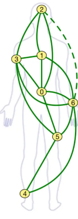
The set of links that most protocols rely on is represented on Fig. 4. The link between the head and the wrist exists, but is seldom used.

4.2.2. Setting the maximum Time-To-Live

The Time-To-Live (TTL) mechanism limits packets retransmissions independently of the broadcast algorithm. A high TTL value results in a huge number of packets traveling in the network, ultimately provoking queueing and collisions, while a low value limits the decision power of the different algorithms. Setting this value in a low diameter mobile network may be uneasy, that’s why we rely on simulation results to find a fair value. In our implementation, the TTL is decremented from the first transmission, which means that a packet whose initial TTL value is equal to 1 will only be emitted once and never be forwarded.

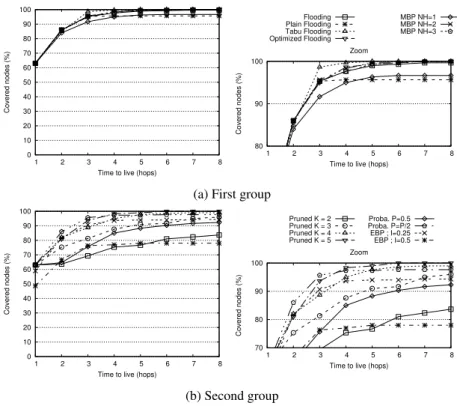
Figure 5 shows the percentage of covered nodes in function of the packets initial TTL in the walking posture. This posture corresponds to a soft and regular motion, in which the source has at least three direct neighbors. When TTL is equal to 1, 63% of the network is covered for

4_{Results for other postures are available online: http://www.chaudet.ch/WBAN/}

(13)

0 10 20 30 40 50 60 70 80 90 100 -60 -50 -40 -30 -20 -10 0 Covered nodes (%) Transmission Power (dBm) 90 100 -60 -58 -56 -54 -52 -50 Covered nodes (%) Transmission Power (dBm) Zoom Flooding Plain Flooding Tabu Flooding Optimized Flooding MBP NH=1 MBP NH=2 MBP NH=3 One hop

(a) Walking posture

0 10 20 30 40 50 60 70 80 90 100 -60 -50 -40 -30 -20 -10 0 Covered nodes (%) Transmission Power (dBm) 50 60 70 80 90 100 -60 -58 -56 -54 -52 -50 -48 -46 Covered nodes (%) Transmission Power (dBm) Zoom (b) Sleeping posture

Figure 2: Percentage of covered nodes in function of Nodes Transmission Power (First Group)

nearly all strategies, except EBP variations. EBP shows a lower performance in this situation due to the amount of control packets that cause collisions on the one hand and the necessity to reach a certain number of neighbors before transmitting a packet on the other hand. With a high Hello frequency the control traffic causes additional delays and collisions, while decreasing this frequency leads to more frequent neighbors timeout expirations.

The strategy Flooding represents a reference, as nothing prevents retransmission as long as the TTL is positive. It therefore achieves a quite high coverage performance in this low-traffic scenario where collisions are unlikely. Plain Flooding has a similar behavior when the TTL is low but fails to improve when the TTL gets greater than 3 because it filters out packets as soon as they have been received once and hence does not benefit from a TTL increase.

For MBP, NH represents the threshold that separates Plain Flooding from acknowledged broadcasting. As soon as NH reaches a value of 2 hops, Figure 5 shows that MBP has a satis-factory performance evolution. Optimized Flooding also shows comparable performance. For example, with T T L = 4, 98.6% of the network is covered. The fact that these strategies both achieve a performance level comparable to Flooding while they prevent packets retransmissions much sooner, indicates that they are able to find the correct compromise between traffic volume and coverage.

For Pruned Flooding strategy, the choice of the number of random receiver among the neigh-bors, K, has a direct influence on the coverage probability. Figure 5 shows results for K varying from 2 to 5 and shows that with K = 2 and K = 3 it is almost impossible to cover all the nodes even with higher values of TTL.

(14)

0 10 20 30 40 50 60 70 80 90 100 -60 -50 -40 -30 -20 -10 0 Covered nodes (%) Transmission Power (dBm) 50 60 70 80 90 100 -60 -58 -56 -54 -52 -50 Covered nodes (%) Transmission Power (dBm) Zoom Pruned K = 2 Pruned K = 3 Pruned K = 4 Pruned K = 5 Proba. P=0.5 Proba. P=P/2 EBP ; I=0.25 EBP ; I=0.5

(a) Walking posture

0 10 20 30 40 50 60 70 80 90 100 -60 -50 -40 -30 -20 -10 0 Covered nodes (%) Transmission Power (dBm) 50 60 70 80 90 100 -60 -58 -56 -54 -52 -50 Covered nodes (%) Transmission Power (dBm) Zoom (b) Sleeping posture

Figure 3: Percentage of covered nodes in function of Nodes Transmission Power (Second Group)

Tabu Floodingstands out even for low TTL value (e.g. 3 or 4). Indeed, with Tabu Flooding, messages are sent to specific and uncovered nodes. Thus, unlike in most flooding strategies, a node receiving a message will neither consider, nor forward it unless it is among the list of uncovered nodes. With fewer forwarding events, this protocol is able to better sustain low TTL values, at least in an "easy" position such as walking.

The Probabilistic Flooding (P=P/2) strategy shows a good network coverage starting with TTL value equals to 2. Comparing these results with Probabilistic Flooding (P=0.5), the im-portance of the first emission of the packet appears clearly. This strategy behaves initially as a regular flooding algorithm, with an agressive diffusion, and then, by dividing P by 2, reduces forwarded message copies, thus limiting the induced load.

For the rest of this work, we chose to set the TTL to an initial value of 6 hops, as some strategies are able to reach full network coverage with this value.

4.3. Performance comparison – single packet broadcast

For our first set of evaluations, we chose to examine the scenario on which the gateway only transmits a single broadcast packet. This elementary scenario allows to isolate the protocol behavior without any interaction between successive packets. We compare the different strategies with respect to the following criteria:

• Network Coverage: we evaluate the number of nodes that have received the message at least once and present results as the percentage of covered nodes.

(15)

0 1 2 3 4 5 6

Figure 4: Set of links used by the protcols when the emission power is set to -55 dBm

• Latency: we display the average end-to-end delay from the source to reach its last desti-nation (i.e. the last node successfully covered).

• Traffic Load: as a indicator of energy consumption, we evaluate the total number of trans-missions and receptions realized by all nodes in the network, assuming that communication is the main source of energy consumption that protocols have an influence on.

Some strategies rely on specific key parameters which have an influence on their perfor-mance. To understand these parameters impact, we run simulations with different configurations:

• MBP: the threshold on the number of hops NH varies between 1 and 3 hops. • EBP: the inter-hello messages interval, I, varies between I= 0.25 s and I = 0.5 s • Pruned Flooding: the number of next hops, K, varies between 2 and 5 nodes. 4.3.1. Network Coverage

Figure 6 presents the percentage of covered nodes per posture. Looking at these figures, we can clearly distinguish two group of strategies.

The first group, which includes Tabu Flooding, Pruned Flooding for K= 5 and K = 4, Op-timized Flooding, Flooding and MBP when NH = 2 and NH = 3, exhibits good performance, close to 100 % coverage in almost all situations. These protocols are able to handle most situa-tions correctly, with the notable exception of the sleep position that turns out to be challenging for these protocols who barely achieve 90 % coverage.

(16)

0 10 20 30 40 50 60 70 80 90 100 1 2 3 4 5 6 7 8 Covered nodes (%)

Time to live (hops)

80 90 100

1 2 3 4 5 6 7 8

Covered nodes (%)

Time to live (hops) Zoom Flooding Plain Flooding Tabu Flooding Optimized Flooding MBP NH=1 MBP NH=2 MBP NH=3

(a) First group

0 10 20 30 40 50 60 70 80 90 100 1 2 3 4 5 6 7 8 Covered nodes (%)

Time to live (hops)

70 80 90 100 1 2 3 4 5 6 7 8 Covered nodes (%)

Time to live (hops) Zoom Pruned K = 2 Pruned K = 3 Pruned K = 4 Pruned K = 5 Proba. P=0.5 Proba. P=P/2 EBP ; I=0.25 EBP ; I=0.5 (b) Second group

Figure 5: Percentage of covered nodes in function of TTL in the walk posture

The second group, composed of Pruned Flooding for K = 2 and K = 3, EBP for I = 0.5, Plain Floodingand Probabilistic Flooding (P=0.5), shows a disappointing performance in all situations. These protocols, or this set of parameters for Pruned Flooding, are not suited to this type of network and/or mobility.

In between these two large clusters, protocols like MBP for NH= 1 or EBP for I = 0.25 s, or Probabilistic Flooding (P=P/2) have a fair performance, except in the case of the sleep position in which they are, however, more stable than some algorithms belonging to the first group. In the case of MBP, messages are delayed and the individual transmission turn out to be well scheduled, reducing collusions and limiting useless forwarding, increasing in turn the chance to reach other nodes. EBP is very sensitive to its inter-hello interval. A smaller value (I == 0.25 s) induces more load on the network and provoke more collisions than a larger value, but makes it easier to discover the neighborhood and hence allows more transmission attempts.

The performance of Probabilistic Flooding (P=P/2) stresses out the importance of the first transmission of each packet. When compared to Plain Flooding, it shows however that it is however not entirely sufficient, as further improvement results from the subsequent transmission attempts.

4.3.2. Latency

Figure 7 represents the average over all postures of the end-to-end delay, i.e. the time required for the first instance of the message to reach each node. Figure 8 shows the average time required to complete the broadcast, i.e. the minimum time to reach every node in the network, per posture.

(17)

0 20 40 60 80 100

Pruned K=2EBP I=0.5Proba. P=0.5Pruned K=3

Plain FloodingEBP I=0.25MBP NH=1Proba. P=P/2MBP NH=2

Flooding_Optimized

MBP NH=3Pruned K=4Pruned K=5

Tabu

Uncovered nodes (%)

(a) Walking posture

0 20 40 60 80 100

Flooding_Optimized MBP NH=3Pruned K=4Pruned K=5 Tabu Covered nodes (%) (b) Running posture 0 20 40 60 80 100

Pruned K=2EBP I=0.5_{Proba. P=0.5}Pruned K=3

Flooding_Optimized

Tabu

Covered nodes (%)

(c) Walking weakly posture

0 20 40 60 80 100

Flooding_Optimized MBP NH=3Pruned K=4Pruned K=5 Tabu Covered nodes (%) (d) Sitting posture 0 20 40 60 80 100

Flooding_Optimized

Tabu

Covered nodes (%)

(e) Lie posture

0 20 40 60 80 100

Flooding_Optimized MBP NH=3Pruned K=4Pruned K=5 Tabu Covered nodes (%) (f) Sleep posture 0 20 40 60 80 100

Flooding_Optimized

Tabu

Covered nodes (%)

(g) Wear posture

Figure 6: Percentage of covered nodes per posture

(18)

We can identify in Fig. 7 a first group of nodes, composed of the navel, head and upper-arm nodes, which are easy to reach, except for EBP. These nodes are the direct neighbors of the gate-way node (located on the chest) and the influence of the protocol is marginal in these situations. EBPneeds to acquire and refresh knowledge of the nodes before it takes the decision to transmit a message and waits for the sufficient number of neighbors to be present simultaneously before attempting a transmission. This precaution has a cost in terms of latency which appears in the different postures. We can however notice that for most postures, results are comparable, even in presence of highly variable links. The only really challenging posture is sleep, in which some links are obstructed for long periods, a situation that protocols that wait for enough neighbors to be present cannot handle properly.

Nodes located on the wrist, ankle or thigh are, in most cases, at least two hops away from the source node, which explains the latency increase. For these nodes we can again distinguish two groups of strategies: MBP when NH ≤ 2, Plain Flooding, Pruned Flooding for K= 2 or K = 3, EBPand Probabilistic Flooding (P=0.5 or P=P/2) generally cause larger delays.

MBPfor NH= 3, Optimized Flooding, Pruned Flooding for K ≥ 4 and Flooding exhibit low delays in most situations. Flooding is the most verbose alternative and always achieves the best performance, as the global network load is not sufficient to cause congestion. Optimized Flooding and MBP both start the diffusion as Plain Flooding, which explains their good performance. Optimized Floodingis a bit more adaptable and ultimately reaches a shorter latency than MBP. Pruned Floodingfor K = 4 also has a behavior close to Flooding due to the network average degree.

Tabu Floodinghas a fair performance. As it targets uncovered nodes, these nodes rapidly become a search target for multiple nodes and the probability that the meet one node ready to transmit the packet to them is large.

4.3.3. Traffic Load and Energy Consumption

We measured the load induced by the different strategies as the total number of emissions and receptions for each node. This measure, which does not include overhearing not only gives an idea of the wireless channel occupancy, but also of the energy consumption – comparable energy being spent for emission and reception of packets – and of the level of electromagnetic energy that wearers are exposed to. Figure 9 compares the total number of emissions and recep-tions per node for all the studied algorithms and Figure 10 shows these figures for each posture. These figures only compare the volume of data packets, leaving aside the control traffic (Hello, acknowledgments, ...)

These figures show, without surprise, that nodes closer to the chest, including the chest itself, are more solicited than peripheral nodes, as they are more natural forwarders and have more active neighbors on average. Comparing the postures, we can notice that most protocols are strongly influenced by the network dynamics, as the number of transmissions increases rapidly with the links variance.

We can categorize once again the different algorithms in three clusters. A first cluster, com-posed of Pruned Flooding for K ≥ 3, Tabu Flooding and Flooding, gathers the most verbose protocols. These protocols, trade their good performance in terms of coverage and latency for a high number of transmissions and receptions. Pruned Flooding and Tabu Flooding even incur more traffic than Flooding, as they decompose the broadcast into multiple unicast transmissions to target specific, uncovered or random, nodes. For example, for Pruned Flooding when K= 3, each received message generates three copies to be forwarded.

(19)

0 0.1 0.2 0.3 0.4 0.5 EBP 2EBP 1 Pruned K=2MBP NH=1_{Proba P=0.5}Pruned K=3

Plain FloodingProba P=P/2MBP NH=2

Flooding_Optimized

Tabu

Latency (s)

(a) Navel node

0 0.2 0.4 0.6 0.8 1 EBP 2EBP 1 Pruned K=2MBP NH=1_{Proba P=0.5}Pruned K=3

Flooding_Optimized MBP NH=3Pruned K=4Pruned K=5 Tabu Latency (s) (b) Head node 0 0.2 0.4 0.6 0.8 1 1.2 1.4 1.6 1.8 EBP 2EBP 1 Pruned K=2MBP NH=1_{Proba P=0.5}Pruned K=3

Flooding_Optimized MBP NH=3Pruned K=4Pruned K=5 Tabu Latency (s) (c) Ankle node 0 0.2 0.4 0.6 0.8 1 1.2 1.4 1.6 1.8 EBP 2EBP 1 Pruned K=2MBP NH=1_{Proba P=0.5}Pruned K=3

Flooding_Optimized

Tabu

Latency (s)

(d) Upper arm node

0 0.2 0.4 0.6 0.8 1 1.2 1.4 1.6 1.8 EBP 2EBP 1 Pruned K=2MBP NH=1_{Proba P=0.5}Pruned K=3

Flooding_Optimized

Tabu

Latency (s)

(e) Thigh node

Flooding_Optimized

Tabu

Latency (s)

(f) Wrist node

Figure 7: Latency per Node

A second group, composed by Plain Flooding, Probabilistic Flooding (P=0.5 or P=P/2), MBPfor NH ≤ 2 and Optimized Flooding, are usually relatively silent. They require about 3 times less transmissions than Flooding, but pay this low traffic volume with a reduced perfor-mance, except for Optimized Flooding which achieves a good compromise.

Between these two extremes, protocols like EBP, MBP for NH = 3 or Pruned Flooding for K= 2 generate moderate traffic in most situations.

(20)

Flooding_Optimized

Tabu

Latency (s)

(a) Walking posture

Flooding_Optimized MBP NH=3Pruned K=4Pruned K=5 Tabu Latency (s) (b) Running posture 0 0.1 0.2 0.3 0.4 0.5 EBP 2EBP 1 Pruned K=2MBP NH=1_{Proba P=0.5}Pruned K=3

Flooding_Optimized

Tabu

Latency (s)

Flooding_Optimized MBP NH=3Pruned K=4Pruned K=5 Tabu Latency (s) (d) Sitting posture 0 0.1 0.2 0.3 0.4 0.5 EBP 2EBP 1 Pruned K=2MBP NH=1Proba P=0.5Pruned K=3

Flooding_Optimized

Tabu

Latency (s)

(e) Lie posture

0 0.5 1 1.5 2 2.5 3 3.5 4 4.5 EBP 2EBP 1 Pruned K=2MBP NH=1Proba P=0.5Pruned K=3

Flooding_Optimized MBP NH=3Pruned K=4Pruned K=5 Tabu Latency (s) (f) Sleep posture 0 0.2 0.4 0.6 0.8 1 EBP 2EBP 1 Pruned K=2MBP NH=1_{Proba P=0.5}Pruned K=3

Flooding_Optimized

Tabu

Latency (s)

(g) Wear posture

Figure 8: Latency per posture

(21)

0 10 20 30 40 50 60 70 Pruned K=5Pruned K=4 Tabu Flooding Pruned K=3 EBP 1EBP 2

MBP NH=3Pruned K=2OptimizedMBP NH=2_{Proba P=P/2}MBP NH=1_{Proba P=0.5} Plain Flooding

Number of transmissions/receptions

(a) Navel node

0 10 20 30 40 50 60 70 Pruned K=5Pruned K=4 Tabu Flooding Pruned K=3 EBP 1EBP 2

MBP NH=3Pruned K=2OptimizedMBP NH=2_{Proba P=P/2}MBP NH=1_{Proba P=0.5} Plain Flooding Number of transmissions/receptions (b) Head node 0 5 10 15 20 25 30 Pruned K=5Pruned K=4 Tabu Flooding Pruned K=3 EBP 1EBP 2

MBP NH=3Pruned K=2OptimizedMBP NH=2_{Proba P=P/2}MBP NH=1_{Proba P=0.5} Plain Flooding Number of transmissions/receptions (c) Ankle node 0 10 20 30 40 50 60 70 Pruned K=5Pruned K=4 Tabu Flooding Pruned K=3 EBP 1EBP 2

(d) Upper arm node

0 10 20 30 40 50 Pruned K=5Pruned K=4 Tabu Flooding Pruned K=3 EBP 1EBP 2

MBP NH=3Pruned K=2OptimizedMBP NH=2_{Proba P=P/2}MBP NH=1Proba P=0.5_{Plain Flooding}

(e) Thigh node

0 10 20 30 40 50 60 70 80 Pruned K=5Pruned K=4 Tabu Flooding Pruned K=3 EBP 1EBP 2

Number of transmissions/receptions (f) Wrist node 0 10 20 30 40 50 60 70 80 Pruned K=5Pruned K=4 Tabu Flooding Pruned K=3 EBP 1EBP 2

(g) Chest node

Figure 9: Traffic load per Node

(22)

0 100 200 300 400 500 600 700 800 Pruned K=5Pruned K=4 Tabu Flooding Pruned K=3 EBP 1EBP 2

(a) Walking posture

0 100 200 300 400 500 600 Pruned K=5Pruned K=4 Tabu Flooding Pruned K=3 EBP 1EBP 2

MBP NH=3Pruned K=2OptimizedMBP NH=2_{Proba P=P/2}MBP NH=1_{Proba P=0.5} Plain Flooding Number of transmissions/receptions (b) Running posture 0 200 400 600 800 1000 1200 Pruned K=5Pruned K=4 Tabu Flooding Pruned K=3 EBP 1EBP 2

0 200 400 600 800 1000 Pruned K=5Pruned K=4 Tabu Flooding Pruned K=3 EBP 1EBP 2

MBP NH=3Pruned K=2OptimizedMBP NH=2_{Proba P=P/2}MBP NH=1_{Proba P=0.5} Plain Flooding Number of transmissions/receptions (d) Sitting posture 0 100 200 300 400 500 Pruned K=5Pruned K=4 Tabu Flooding Pruned K=3 EBP 1EBP 2

(e) Lie posture

0 50 100 150 200 Pruned K=5Pruned K=4 Tabu Flooding Pruned K=3 EBP 1EBP 2

Number of transmissions/receptions (f) Sleep posture 0 50 100 150 200 250 300 350 400 Pruned K=5Pruned K=4 Tabu Flooding Pruned K=3 EBP 1EBP 2

(g) Wear posture

Figure 10: Traffic load per posture

(23)

4.4. Summary

Table 2 reports the average values for all simulation, all nodes and all postures per protocol for one single packet transmission. We can classify, from these figures, protocols in 4 groups. The first group, containing EPB and Pruned Flooding for K = 2 and K = 3 has disappointing performance. The second group, with MBP (NH= 1), Probabilistic Flooding (P=0.5) and Plain Floodinghas a non-satisfying performance but generates little traffic. The third group, containing Pruned Flooding(K= 4 and 5), Tabu Flooding and Flooding trades traffic load for performance. Finally, the fourth group, including MBP (NH= 2, NH = 3), Probabilistic Flooding (P=P/2) and Optimized Floodingrealized a fair compromise between all these aspects.

Coverage Latency Traffic (%) (ms) (pkt) EBP I= 0.5 s 86.3 808.6 64.3 EBP I= 0.25 s 91.0 541.9 69.0 Pruned FloodingK= 2 77.5 235.2 59,9 MBPNH= 1 95.7 169.5 24 Probabilistic Flooding (P=0.5) 87.6 132.3 26.1 Pruned FloodingK= 3 89.8 121.0 134.9 Plain Flooding 90.2 104.7 14.7 MBPNH= 2 97.2 85.4 36.0 Pruned FloodingK= 4 96.7 59,9 239.9 Probabilistic Flooding (P=P/2) 95.0 58,1 30.8 MBPNH= 3 97.7 47.9 53.8 Tabu Flooding 97.5 47.6 133.8 Pruned FloodingK= 5 98.7 42.5 396.6 Optimized Flooding 97.0 39.3 39.9 Flooding 97.8 31.6 119.2

Table 2: Average Network coverage, latency and traffic load for all protocols

5. Increasing Traffic Load

In this set of simulations, we progressively increase the traffic load to evaluate how protocols react under different traffic conditions. When the load increases, packets may either be dropped before being emitted due to a full MAC-level queue, or get emitted but be lost to some receivers because of collisions and congestion may prevent some nodes to access the medium. In all cases, some packets will never reach their destination, or be received through alternate, usually longer, paths, which may disrupt the packets reception order.

In this section, we gradually increase the packets load from 2 packets/s to 1000 packets/s. Each packet is 544 bits long and the medium capacity is 250 kbit/s. If the resulting load becomes clearly unrealistic with respect to classical WBAN applications, it allows us to characterize the global behavior and to detect tripping points. The MAC buffer size is set to 100 packets. 5.1. Network Coverage

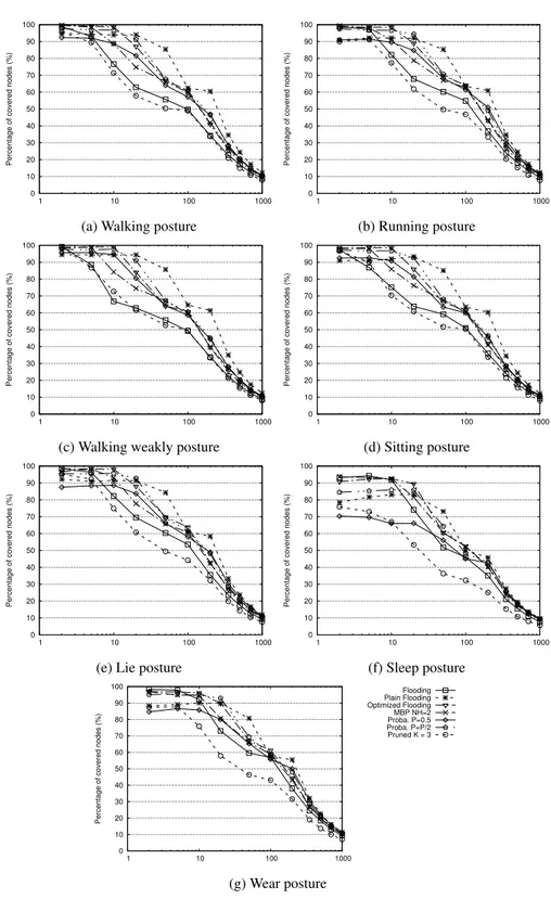
Figure 11 presents the average proportion of nodes covered over all packets, when the emis-sion throughput increases. This measure allows us to see how reliable the different protocols are under different loads.

(24)

We can notice that all protocols have the same behavior: starting from a few packets per second, which depends on the protocol (5 for MBP and Flooding; 10 for Optimized Flooding and Probabilistic Flooding (P=0.5 or P=P/2)) and on the posture, the percentage decreases rapidly to converge to similar values, around 10 %. The protocols classification is similar for all postures: Plain Floodingand Optimized Flooding resist slightly better, followed by Probabilistic Flooding (P=0.5 or P=P/2). The Pruned Flooding and Flooding strategies have the worst scalability. This classification follows the different approaches verbosity: the protocols that tend to let numerous copies of the same packet travel in the network have lower scalability when compared to more cautious protocols. There is no real effect of the posture on the general behavior of the different protocols, however the initial performance and the tripping point are different in function of the nodes relative mobility.

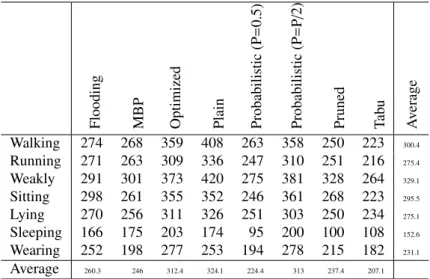
Table 3 reports the number of packets successfully received by all the nodes in the different postures for different protocols in the scenario where the source emits a saturating throughput of 1000 packets/s. We let emitter generate 10000 packets, most of which are dropped in the sender’s queue, as the wireless channel cannot sustain such a load. Figures reported in the table are the average over 50 simulations for each scenario.

These figures confirm that sleeping is, by far, the most challenging position for the different protocols, followed by wearing jacket. Concerning protocols, Flooding, MBP, Pruned Flooding, Probabilistic Flooding (P=0.5) and Tabu Flooding have lower success rates than Plain Flood-ing, Probabilistic Flooding (P=P/2) and Optimized Flooding. This indicates that neither the too verbose solutions nor the ones that rely on neighbors identification deal correctly with a high load, which is logical as both families generate a high data or control traffic. Indeed, the good ranking of Plain Flooding even suggests that a single transmission from all nodes is sufficient in most positions, except for Sleep where Optimized Flooding behaves slightly better.

Flooding MBP Optimized Plain Probabilistic

(P = 0.5) Probabilistic (P = P/ 2) Pruned Tab u A v erage Walking 274 268 359 408 263 358 250 223 300.4 Running 271 263 309 336 247 310 251 216 275.4 Weakly 291 301 373 420 275 381 328 264 329.1 Sitting 298 261 355 352 246 361 268 223 295.5 Lying 270 256 311 326 251 303 250 234 275.1 Sleeping 166 175 203 174 95 200 100 108 152.6 Wearing 252 198 277 253 194 278 215 182 231.1 Average 260.3 246 312.4 324.1 224.4 313 237.4 207.1

Table 3: Number of successfully broadcasted packets in function of the posture – saturated scenario

Table 4 reports the number of distinct packets received by each node, averaged over 50 sim-ulations and over all positions, truncated to 1 digit. The value for chest represents the number of packets that are received back from neighbors forwarding and may does not have any application-level meaning. This confirms that the most difficult nodes to reach are the ones located at least

(25)

0 10 20 30 40 50 60 70 80 90 100 1 10 100 1000

Percentage of covered nodes (%)

(a) Walking posture

0 10 20 30 40 50 60 70 80 90 100 1 10 100 1000

(b) Running posture 0 10 20 30 40 50 60 70 80 90 100 1 10 100 1000

0 10 20 30 40 50 60 70 80 90 100 1 10 100 1000

(d) Sitting posture 0 10 20 30 40 50 60 70 80 90 100 1 10 100 1000

(e) Lie posture

0 10 20 30 40 50 60 70 80 90 100 1 10 100 1000

(f) Sleep posture 0 10 20 30 40 50 60 70 80 90 100 1 10 100 1000

Flooding Plain Flooding Optimized Flooding MBP NH=2 Proba. P=0.5 Proba. P=P/2 Pruned K = 3 (g) Wear posture

Figure 11: Percentage of covered nodes per posture

(26)

two hops away from the source (Ankle and thigh). Here we can see that Plain Flooding is the most efficient protocol when it comes to reaching these "difficult" nodes, followed by Probabilis-tic Flooding (P=P/2) and Optimized Flooding.

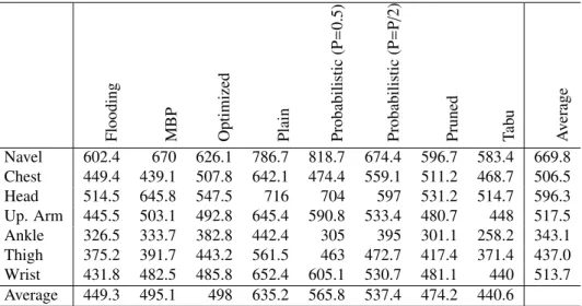
(P = 0.5) Probabilistic (P = P/ 2) Pruned Tab u A v erage Navel 602.4 670 626.1 786.7 818.7 674.4 596.7 583.4 669.8 Chest 449.4 439.1 507.8 642.1 474.4 559.1 511.2 468.7 506.5 Head 514.5 645.8 547.5 716 704 597 531.2 514.7 596.3 Up. Arm 445.5 503.1 492.8 645.4 590.8 533.4 480.7 448 517.5 Ankle 326.5 333.7 382.8 442.4 305 395 301.1 258.2 343.1 Thigh 375.2 391.7 443.2 561.5 463 472.7 417.4 371.4 437.0 Wrist 431.8 482.5 485.8 652.4 605.1 530.7 481.1 440 513.7 Average 449.3 495.1 498 635.2 565.8 537.4 474.2 440.6

Table 4: Number of successfully received packets in per node – saturated scenario ; all postures average

5.2. Drop causes

TableFigure 5 reports the number of dropped packets due to collisions and busy channel (drop before sending) per posture and Table 6 reports the same figure per node, averaged over the postures. First, it is worth noting that collisions and medium load evolve together, whihc is expected on a single channel. Comparing protocols, these results are coherent with the other statistics: verbose protocols such as Flooding, Tabu Flooding, Pruned Flooding and MBP are more prone to increase the medium load. Plain Flooding and Probabilistic Flooding (P=0.5 or P=P/2), on the opposite, have a lighter impact on the channel occupancy, while Optimized Floodinggenerates a quite high load. Concerning positons, the amount of collision is lower in positions whose success rate is low, which indicates that the success rate is more related to reachability of the nodes than to an excessive collisions amount.

When breaking down the drops per node, even if we can see variations among the nodes, the volume of collisions and packets dropped after failing to access the channel remains relatively uniform across the network. We can notice that central nodes suffer from relatively low collisions level even if they are relatively more prone to suffer from a busy channel. This can be explained by the fact that that these nodes act more often as emitters than the others. The wrist node appears to be suffering from both effects, while the ankle node appears more isolated. The head, upper arm have different but average profiles.

5.3. Unnecessary traffic load

Table 7 reports the average number of redundant copies of each packet received by each node. These figures are the average over 50 simulations and over all postures. We can see there that nodes which are direct neighbors of the source, such as the navel, but also the chest, head

(27)

Flooding MBP Optimized Plain Probabilistic (P = 0.5) Probabilistic (P = P/ 2) Pruned Tab u A v erage Walking Collisions 965.6 808.6 748.1 471.1 455.6 628.4 774.2 750.7 700.3 Busy channel 56.5 38.5 43.0 17.0 19.8 33.6 46.5 41.6 37.1 Running Collisions 950.0 865.7 716.6 476.1 412.9 608.5 806.4 830.0 708.3 Busy channel 43.5 29.2 31.9 12.6 11.7 23.6 37.9 35.6 28.3 Weakly Collisions 1048.5 858.4 832.6 495.4 537.3 684.9 898.4 870.2 778.2 Busy channel 64.1 45.9 51.0 19.9 27.5 40.0 56.2 50.6 44.4 Sitting Collisions 859.8 762.9 702.0 424.6 434.7 586.6 738.0 720.4 653.6 Busy channel 54.0 38.9 44.4 16.5 22.5 35.5 47.7 42.2 37.7 Lying Collisions 897.2 812.9 682.5 461.2 395.4 587.2 777.5 808.9 677.8 Busy channel 38.8 24.5 28.1 11.5 11.0 21.5 35.5 33.3 25.5 Sleeping Collisions 632.0 683.0 535.5 422.2 287.0 487.9 674.2 763.8 560.7 Busy channel 15.9 14.4 9.6 4.4 3.1 7.4 14.8 19.4 11.1 Wearing Collisions 878.6 794.5 696.3 499.2 389.6 612.3 777.4 888.5 692.1 Busy channel 27.2 17.7 20.7 9.6 6.7 16.0 26.0 29.5 19.2 Average Collisions 890.3 798.0 701.9 464.3 416.1 599.4 778.0 804.6 Busy channel 42.9 29.9 32.7 13.1 14.6 25.4 37.8 36.1

Table 5: Drop causes per posture

and upper arm, are more exposed than the others. These figures are somehow coherent with the successful packets ratio presented in Table 4, which seems to indicate that the nodes seeing the most traffic are also the better covered ones, yet the figures for the chest node, for instance, or the head node do not follow this pattern. Chest ranks 5th in terms of coeverage but 2nd in terms of redundant receptions, while head and, to a smaller extent, wrist are often covered and only experience moderate redundant receptions.

When it comes to protocols comparison, we can conform our previous conclusions: Flood-ingand Tabu Flooding are very verbose followed by MBP and Pruned Flooding, while Plain Floodingand Probabilistic Flooding (P=0.5 or P=P/2) are the most silent alternatives. Opti-mized Floodingscores fairly. Compared to the one single packet scenario, we can notice that Tabu Floodingused to have a good performance in terms of traffic load and now scales poorly due to the decomposition of the broadcast into multiple unicast transmissions.

5.4. Packets sequencing

Figure 12 presents the average per node of the proportion of de-sequenced packets, i.e. pack-ets that manage to reach the different nodes in the network, but after a subsequent packet has already been received.

In all cases, we can notice three phases: first the different protocols start experiencing out-of-order packets at a proportion that increases from 5 to 10 packets per seconds, depending on the

(28)

Flooding MBP Optimized Plain Probabilistic (P = 0.5) Probabilistic (P = P/ 2) Pruned Tab u A v erage Navel Collisions 834.9 681.1 635.3 390.4 358.0 528.5 695.9 728.2 606.5 Busy channel 50.7 35.0 40.6 17.9 19.9 31.8 46.1 42.2 35.5 Chest Collisions 840.5 732.9 644.5 369.9 317.2 527.3 747.3 823.9 625.4 Busy channel 57.7 36.6 46.0 13.8 20.3 35.1 53.6 45.3 38.5 Head Collisions 800.9 859.7 634.6 425.3 393.6 549.1 697.7 707.1 633.5 Busy channel 45.8 26.7 35.7 15.3 15.8 27.4 41.2 38.5 30.8 Up. Arm Collisions 939.1 767.2 742.6 516.5 454.1 645.5 798.7 817.3 710.1 Busy channel 51.9 36.4 38.8 15.9 17.5 30.2 44.5 44.0 34.9 Ankle Collisions 767.4 827.9 611.0 389.0 388.8 515.5 726.1 696.4 615.3 Busy channel 5.2 3.4 3.4 1.7 1.5 2.8 3.5 5.0 3.3 Thigh Collisions 988.8 852.5 808.8 575.3 501.7 706.1 881.2 909.5 778.0 Busy channel 29.5 28.1 20.4 8.9 8.2 16.5 23.8 26.5 20.2 Wrist Collisions 1060.2 864.6 836.8 583.5 499.2 723.9 899.3 950.0 802.2 Busy channel 59.3 42.9 43.7 18.1 19.1 33.8 52.0 50.8 40.0 Average Collisions 890.3 798.0 701.9 464.3 416.1 599.4 778.0 804.6 Busy channel 42.9 29.9 32.7 13.1 14.6 25.4 37.8 36.1

Table 6: Drop causes per Node

(P = 0.5) Probabilistic (P = P/ 2) Pruned Tab u A v erage Navel 92.7 4.2 26.2 6.2 19.7 15 29.1 92.5 35.7 Chest 51.2 8 5.7 3.7 4.7 3.8 48.5 23.8 18.7 Head 24.2 20.4 20.7 3.5 7.4 6.5 18 17 14.7 Up. Arm 29.2 30 9.2 2.1 14.7 7.1 21.4 34.2 18.5 Ankle 7 26.2 9 4 1.1 2.7 7.8 21.5 9.9 Thigh 19 29.7 5.1 1.4 4.1 2.2 6.1 23.4 11.4 Wrist 14 16.4 8.2 3.8 5.7 7.2 17.5 29 12.7 Average 33.9 19.3 12.0 3.5 8.2 6.4 21.2 34.5

Table 7: Number of redundant receptions per node – saturated scenario ; all postures average