Behavioral Application-dependent superscolor core modeling

(1)

HAL Id: tel-00942289

https://tel.archives-ouvertes.fr/tel-00942289

Submitted on 5 Feb 2014

HAL is a multi-disciplinary open access archive for the deposit and dissemination of sci-entific research documents, whether they are pub-lished or not. The documents may come from teaching and research institutions in France or abroad, or from public or private research centers.

L’archive ouverte pluridisciplinaire HAL, est destinée au dépôt et à la diffusion de documents scientifiques de niveau recherche, publiés ou non, émanant des établissements d’enseignement et de recherche français ou étrangers, des laboratoires publics ou privés.

modeling

Ricardo Andrés Velásquez Vélez

To cite this version:

Ricardo Andrés Velásquez Vélez. Behavioral Application-dependent superscolor core modeling. Other [cs.OH]. Université Rennes 1, 2013. English. �NNT : 2013REN1S100�. �tel-00942289�

(2)

ANNÉE 2013

THÈSE / UNIVERSITÉ DE RENNES 1

sous le sceau de l’Université Européenne de Bretagne

pour le grade de

DOCTEUR DE L’UNIVERSITÉ DE RENNES 1

Mention : INFORMATIQUE

École doctorale Matisse

présentée par

Ricardo Andrés V

ELÁSQUEZ

V

ÉLEZ

préparée à l’unité de recherche INRIA – Bretagne Atlantique

Institut National de Recherche en Informatique et Automatique

ISTIC

Behavioral

Application-dependent

Superscalar

Core Modeling

Thèse soutenue à Rennes le 19 April 2013

devant le jury composé de :

Smail NIAR

Professeur à l’Université de Valenciennes / Rapporteur

Lieven EECKHOUT

Professeur à l’Université de Gent/ Rapporteur

Frédéric PÉTROT

Professeur à l’Institut Polytechnique de Grenoble /

Examinateur

Steven DERRIEN

Professeur à l’université de Rennes 1/ Examinateur

André SEZNEC

Directeur de recherche à l’INRIA /Directeur de thèse

Pierre MICHAUD

(3)

(4)

2.3 Simulation methodologies . . . 18 2.3.1 Workload design . . . 18 2.3.1.1 Single-program workloads . . . 19 2.3.1.2 Multiprogram workloads . . . 20 2.3.2 Sampling simulation . . . 21 2.3.2.1 Statistical sampling . . . 21 2.3.2.2 Representative Sampling . . . 22 2.3.3 Statistical simulation . . . 23 2.4 Performance metrics . . . 24 2.4.1 Single-thread workloads . . . 24 1

(5)

2.4.2 Multi-thread workloads . . . 25

2.4.3 Multiprogram workloads . . . 25

2.4.3.1 Prevalent metrics . . . 25

2.4.3.2 Other metrics . . . 26

2.4.4 Average performance . . . 26

3 Behavioral Core Models 29 3.1 Introduction . . . 29

3.2 The limits of approximate microarchitecture modeling . . . 31

3.3 The PDCM behavioral core model . . . 33

3.3.1 PDCM simulation flow . . . 34

3.3.2 Adapting PDCM for detailed OoO core . . . 34

3.3.2.1 TLB misses and inter-request dependencies . . . 35

3.3.2.2 Write-backs . . . 36

3.3.2.3 Branch miss predictions . . . 36

3.3.2.4 Prefetching . . . 36

3.3.2.5 Delayed hits . . . 37

3.3.3 PDCM limitations . . . 38

3.4 BADCO: a new behavioral core model . . . 38

3.4.1 The BADCO machine . . . 39

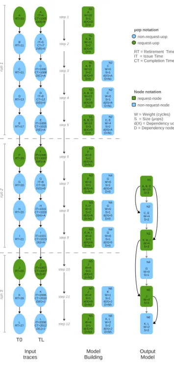
3.4.2 BADCO model building . . . 41

3.5 Experimental evaluation . . . 43

3.5.1 Metrics . . . 43

3.5.2 Quantitative accuracy . . . 45

3.5.3 Qualitative accuracy . . . 45

3.5.4 Simulation speed . . . 47

3.6 Modeling multicore architectures with BADCO . . . 49

3.6.1 Experimental setup . . . 50

3.6.2 Experimental results . . . 51

3.6.3 Multicore simulation speed . . . 52

3.7 Summary . . . 54

4 Multiprogram Workload Design 55 4.1 Introduction . . . 55

4.2 The problem of multiprogram workload design . . . 56

4.3 Random sampling . . . 57

4.4 Experimental evaluation . . . 59

4.4.1 Simulation setup . . . 59

4.5 Experimental results for random sampling . . . 60

4.5.1 Random sampling model validation . . . 60

4.5.2 Performance difference impacts the sample size . . . 61

(6)

Contents 3

4.6 Alternative sampling methods . . . 64

4.6.1 Balanced random sampling . . . 64

4.6.2 Stratified random sampling . . . 65

4.6.2.1 Benchmark stratification . . . 66

4.6.2.2 Workload stratification . . . 67

4.6.3 Actual degree of confidence . . . 67

4.7 Practical guidelines in multiprogram workload selection . . . 68

4.7.1 Simulation overhead: example . . . 69

4.8 Summary . . . 70

5 Conclusion 73 A Résumé en français 77 A.1 Introduction . . . 77

A.2 Contributions . . . 78

A.3 Modèles comportementaux . . . 79

A.3.1 Modèle comportemental PDCM . . . 80

A.3.2 BADCO : un nouveau modèle comportemental . . . 82

A.3.3 Évaluation expérimentale . . . 83

A.3.3.1 Précision simple cœur . . . 83

A.3.3.2 Précision multi-cœur . . . 84

A.3.3.3 Vitesse de simulation . . . 85

A.4 Sélection de charges de travail multiprogrammées . . . 86

A.4.1 Méthodes d’échantillonnage . . . 87

A.4.1.1 Échantillonnage aléatoire simple . . . 87

A.4.1.2 Échantillonnage aléatoire équilibré . . . 87

A.4.1.3 Échantillonnage aléatoire stratifié . . . 87

A.4.2 Évaluation expérimentale . . . 88

A.5 Conclusions . . . 89

Bibliography 99

List of Figures 101

(7)

(8)

Chapter 1

Introduction

Many engineering fields allow us to build prototypes that are identical to the target design. They may cost more, but it is still feasible to build them. These prototypes can be tested under normal and extreme conditions. Hence, it is possible to verify that the design works properly and to define its physical limits. However, most other engineering fields make extensive use of simulation. Simulation has brought significant improvements to cars, airplanes, tires, computer systems, etc. If the target complexity remains constant, like in the physical world for example, then the simulation perfor-mance improves as computers get faster. This is not the case for computer systems simulation, because computers’ complexity increases each new generation, and it in-creases faster than computers’ performance. Moreover, the production of prototypes is extremely expensive and time consuming.

In the beginning of the computer age, computer architects relied on intuition and simple models to choose among different design points. Current processors are too complex to trust intuition. Computer architects require proper performance evaluation tools and methodologies to overcome processor complexity, and to make correct design decisions. Simulators allow computer architects to verify their intuition, and to catch issues that were not considered at all or incorrectly. Meanwhile, correct methodologies give confidence and generality to research conclusions.

1.1 Context

In recent years, research in microarchitecture has shifted from single-core to multicore processors. More specifically, the research focus has moved from core microarchitecture to uncore microarchitecture. Cycle-accurate models for many-core processors featuring hundreds or even thousands of cores are out of reach for simulating realistic workloads. A large portion of the simulation time is spend in the cores, and it is this portion that grows linear with every processor generation. Approximate simulation methodologies, which trade off accuracy for simulation speed, are necessary for conducting certain

(9)

research. In particular, they are needed for studying the impact of resource sharing between cores, where the shared resources can be caches, on-chip network, memory bus, power, temperature, etc.

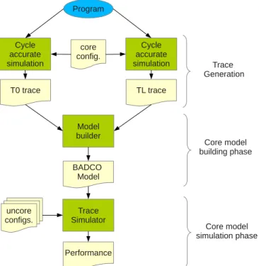
Behavioral superscalar core modeling is a possible way to trade off accuracy for simulation speed in situations where the focus of the study is not the core itself, but what is outside the core, i.e., the uncore. In this modeling approach, a superscalar core is viewed as a black box emitting requests to the uncore at certain times. One or more behavioral core models can be connected to a cycle-accurate uncore model. Behavioral core models are built from detailed simulations. Once the time to build the model is amortized, important simulation speedups can be obtained. Moreover, behavioral core models enable vendors to share core models of its processors in order that third parties can work on specific design of the uncore.

Multicore processors also demand for more advanced and rigorous simulation method-ologies. Many popular methodologies designed by computer architects for simulation of single core architectures must be adapted or even rethought for simulation of multicore architectures. For instance, sampled simulation and its different implementations have been created to reduce the amount of simulation time required, while still providing accurate simulation performance values for single thread programs. However, very few works have focused on how sampled simulation can be applied to multiprogram exe-cution. Furthermore, some of the problems associated with sampled simulation, such as the cold start effect, have not been studied in the context of multicore architecture simulation yet.

An important methodology problem that has not received enough attention is the problem of selecting multiprogram workloads for the evaluation of multicore through-put. The population of possible multiprogram workloads may be very large. Hence, most studies use a relatively small sample of a few tens, or sometimes a few hundreds of workloads. Assuming that all the benchmarks are equally important, we would like this sample to be representative of the whole workload population. Yet, there is no standard method in the computer architecture community for defining multiprogram workloads. There are some common practices, but not really a common method. More important, authors rarely demonstrate the representativeness of their workload samples. Indeed, it is difficult to assess the representativeness of a workload sample without simulating a much larger number of workloads, which is precisely what we want to avoid. Approx-imate microarchitecture simulation methods that trade accuracy for simulation speed offer a solution to this dilemma. We show in this thesis that approximate simulation can help select representative multiprogram workloads for situations that require the accuracy of cycle-accurate simulation.

(10)

Research Questions 7

1.2 Research Questions

Currently, many research studies are focused on multicore processors. The complex-ity of multicore architectures impose a huge challenge to simulation techniques and methodologies. Due to time cost, cycle accurate simulators are out of consideration for tasks such as design space exploration, while approximate simulation exists as an op-tion for faster simulaop-tion, but at the expense of accuracy. Moreover, common simulaop-tion methodologies such as sampling, warming and workload design must be reviewed and updated to target multicore experiments. The aim of this thesis is to provide computer architects with new simulation tools and methodologies that allow for faster and more rigorous evaluation of research ideas on multicore architectures. In particular, we first tackle the problem of slow simulation speed with behavioral core models; and second the problem of selecting multiprogram workloads.

Consequently, the main research questions of the thesis are:

• How, and at what cost, can behavioral core models model realistic superscalar core architectures?

• How, and at what cost, can behavioral core models speed up multicore simulation? • How can we select a representative sample of multiprogram workloads for

perfor-mance evaluation of multicore architectures?

1.3 Contributions

The main contributions of this thesis can be summarized as follows:

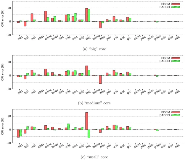
BADCO: a new method for defining behavioral core models We describe and study a new method for defining behavioral models for modern superscalar cores. The proposed Behavioral Application-Dependent Superscalar Core model, BADCO, predicts the execution time of a thread running on a superscalar core with an average error of less than 3.5 % in most cases. We show that BADCO is qualitatively accurate, being able to predict how performance changes when we change the uncore. The simulation speedups we obtained are typically between one and two orders of magnitude.

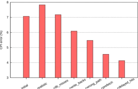
Adapting PDCM to model realistic core architectures We study the PDCM model, a previously proposed behavioral core model, evaluating its accuracy for model-ing modern superscalar core architectures. We identify the approximations that reduce PDCM’s accuracy for modeling realistic architectures. Then, we propose and implement some modifications to the PDCM model core features such as branch miss prediction and prefetch modules in level-1 caches. We reduce the average error from approximately 8 % with the original PDCM, to roughly 4 % with our improved PDCM model.

(11)

Workload stratification: a new methodology for selecting multiprogram work-loads We propose and compare different sampling methods for defining multiprogram workloads for multicore architectures. We evaluate their effectiveness on a case study that compares several multicore last-level cache replacement policies. We show that random sampling, the simplest method, is robust enough to define a representative sample of workloads, provided the sample is big enough. We propose a new method, workload stratification, which is very effective at reducing the sample size in situations where random sampling would require a large sample size. Workload stratification uses approximate simulation for estimating the required sample size.

New analytical model for computing the degree of confidence of random samples Confidence intervals are the most common method to compute the degree of confidence of random samples. We propose an alternative method where the degree of confidence is defined as the probability of drawing correct conclusions when comparing two design points. This analytical method computes the degree of confidence as a function of the sample size and the coefficient of variation. The method can be used either to compute the confidence of a sample or the sample size provided that we can measure the coefficient of variation. We show that an approximate simulator can help in the estimation of the coefficient of variation.

1.4 Thesis Outline

The remainder of this thesis is organized as follows. First, Chapter 2 presents the main theory and techniques related to computer simulation. Chapter 3 presents, evaluates and compares two behavioral core models in the context of single and multicore sim-ulation. Then, Chapter 4 presents and compares different sampling methodologies for selecting multiprogram workloads. Finally, Chapter 5 concludes this thesis by present-ing a summary of contributions, and provides some directions for future work.

(12)

Chapter 2

State of the Art

2.1 Introduction

Many simulation tools and methodologies have been proposed to evaluate the perfor-mance of computer systems accurately. In general, a rigorous perforperfor-mance evaluation for an idea/design implies that a computer architect has to make four important decision: choose the proper modeling/simulation technique, select an adequate baseline configu-ration, define a representative workload sample, and select a meaningful performance metric.

The modeling/simulation technique determines the balance between speed and ac-curacy. In order to overcome the problem of slow simulation tools and huge design space, computer architects use simulation techniques that increase the abstraction level and thus sacrifice accuracy to get speedup. The main simulation techniques include: detailed simulation, analytical modeling, approximate simulation, statistical simulation, sampled simulation, etc. Note that some of these techniques are orthogonal and may be combined.

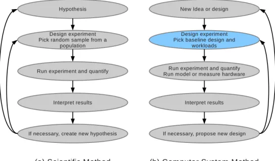
In [24], Eeckhout makes a comparison between the scientific method, in figure 2.1(a), and the computer system method, in figure 2.1(b). He notes that compared to the sci-entific method, the computer method losses rigorousness with selection of the baseline systems and the workload sample. The selection of the baseline system is generally arbi-trary, and in most cases something similar happens with the workload sample selection. Because conclusions may dependent on the baseline systems, the workload sample, or both, the computer method does not guarantee the generality of the conclusions. There is a strong need for making less subjective the task of workload selection. Rigorous performance evaluation is crucial for correct design and for driving research in the right direction.

In this chapter we present the state of the art of prevalent simulation tools and methodologies in the field of computer architecture. The chapter is organized as fol-lows: Section 2.2 presents a taxonomy of computer architecture simulators, and

(13)

Figure 2.1: Scientific method versus computer systems method.

cusses about common techniques to accelerate simulators; Then, Section 2.3 introduces prevalent simulation methodologies; Finally, Section 2.4 describes the most popular throughput metrics.

2.2 Computer architecture simulators

The target of computer simulators is to predict the behavior of computer systems. Gen-erally what we want to predict is timing performance, but other interesting behaviors are: power consumption, energy efficiency, temperature, reliability, yield, etc. Computer architects and software developers use simulators to verify intuitions about changes or new ideas in a computer’s micro/architecture (architects); and new software or software optimizations (software developers).

We want a simulator to be fast, accurate, and easy to expand with new function-alities. A fast simulator enables: wider exploration, deeper exploration, stronger confi-dence and automation. For software development, slowdowns of 10 to 100 are tolerated provided there is enough functionality. For computer architects, accuracy is the most desirable characteristic. However, very often computer architects face the need to trade off accuracy for speed. There are different levels of accuracy depending on the level of abstraction used by the simulator. For example, cycle-accurate simulators exactly match RTL cycle count for performance. It is difficult to quantify which is the minimum level of accuracy tolerated. In general, we want enough accuracy to make comparison and identify tendencies correctly.

(14)

Computer architecture simulators 11

2.2.1 Some simulator terminology

Functional-only simulators only execute the instructions in the target instruction set architecture (ISA) and sometimes emulate some other computer peripherals such as hard-disk, network, usb, etc. Functional-only simulators do not provide timing esti-mates. Many functional-only simulators have evolved into virtual machines, and many others have been extended with temporal models [66, 5, 6]. Functional-only simulators have average slowdowns between 1.25x and 10x depending in the provided functionality [2].

Application simulators or user-level simulators provide basic support for the OS and system calls. Application simulators do not simulate what happens upon an operating system call or interrupt. The most common approach is to ignore interrupts and emulate the effect of system calls [3, 64]. Application simulators have sufficient functionality for some workloads, e.g., SPEC CPU benchmarks spend little time executing system-level code [24].

system simulators give full support of the OS and the peripherals. A Full-system simulator can simulate a whole computer Full-system such that complete software stacks can run on the simulator [24]. Software applications, being simulated in a full-system simulator, have the illusion of running on real hardware. Well-known examples of full-system simulator are SimOS [83], Virtutech’s SimICs [66], AMD’s SimNow [5], etc.

Trace-driven simulators take program instructions and address traces, and feeds the full benchmark trace into a detailed microarchitecture timing simulator [24]. Trace-driven simulators separate functional simulation from timing simulation. The main advantage is that the functional simulation is performed once and can be used to eval-uate performance of many microarchitecture configurations. Some disadvantages of trace-driven simulation include: need for storing the trace files; the impossibility of modeling the effects along mispredicted paths; and impossibility to model the impact of the microarchitecture on inter-thread ordering when simulating multi-thread workloads. driven simulators combine functional with timing simulation. Execution-driven simulators do not have the disadvantages of trace-Execution-driven simulators and are the de-facto simulation approach [24]. The higher accuracy of execution-driven simulators comes at the cost of increased development time and lower simulation speed.

2.2.2 Simulator architectures

The simulator architecture characterizes simulators based on their major internal in-terfaces. These interfaces enable reuse and ease modifications and expansions. The

(15)

selection of the architecture has an impact on the simulator’s speed; the ability to start with a simple model and progressive increase level of detail (accuracy/refinability); the capacity to simulate a wide range of targets (generality); and the amount of work re-quired to write the simulator (effort).

Simulators are software programs characterized by successive state updates of the physical components they model. The way those states are updated may change from simulator to simulator, and depending on the abstraction level. For example, the up-dates can be generated by an approximate model at memory transaction level, or by an RTL model at register level. The number of state updates is correlated with the accuracy and speed of the simulator. Many state updates means higher accuracy and lower simulation speed. In general, computers architects prefer accuracy over speed and system developers prefer speed over accuracy.

A common characteristic among different simulator’s architectures is to split the work in two: functional model (FM) and timing model (TM). The functional model models the instruction set architecture (ISA) and the peripherals; It can execute directly the code or a trace of instructions. The timing model models the performance: number of cycles, power/thermal, reliability, etc. The timing models are approximations to the real counterparts, and the concept of accuracy of a timing simulation is needed to measure the fidelity of these simulators with respect to existing systems.

There exists at least four widely used architectures for cycle-accurate simulators: Integrated [92, 101], Functional-First [78, 2], Timing-First [67], and Timing-Directed [74, 8, 64, 3].

2.2.2.1 Integrated simulation

Integrated simulators model the functionality and the timing together. Hence, there is a single instance for each architectural/micro-architectural state. Such an instance defines the logical and physical behavior. Data paths, timing, functionality must all be correct. If the timing is broken, functionality likely will be broken too. As a consequence, integrated simulators are self-verifying.

In general, integrated simulators require a lot of work and they are also difficult to customize and parallelize. An integrated simulator requires an amount of work equiva-lent to that of an RTL simulator. The accuracy will be also close to RTL simulators but faster. Integration makes this kind of simulators difficult to customize and parallelize. There is a lot of work to make integrated simulators modular [92, 101]. Parallelization is possible in hardware, but then becomes an implementation.

Vachharajani et al. present Liberty Simulation Environment (LSE) [92]. More than a simulator, LSE is a programming model specialized to develop integrated simulators. The main target of LSE is to increase the re-usability of components. LSE abstracts the timing control through stalls. There are two kinds of stall: semantic and structural. Semantic stalls are related to the computation time of the components. Structural stalls are the ones that traditionally occur due to limited resources. LSE automatizes

(16)

the generation of most structural stalls.

PTLsim [101] is a full-system simulator for x86-64 architectures. The level of com-plexity is comparable to an RTL simulator. In order to increase performance and re-usability, PTLsim’s source code provides two libraries: Super Standard Template Library (SuperSTL) and Logic Standard Template Library (logicSTL). LogicSTL is an internally developed add-on to SuperSTL which supports a variety of structures useful for modeling sequential logic. Some of its primitives may look familiar to Verilog or VHDL programmers [100].

2.2.2.2 Functional-first

In a functional-first simulator, the TM fetches instructions from a trace. The trace can be generated on the fly (execution-driven) or it may be stored on disk and piped to the TM (trace-driven). The trace is used to predict the temporal behavior of the target. The TM may back-pressure the FM but otherwise doesn’t have any control over the functional model.

Functional-first simulators enable the FM and TM to be developed and optimized independently. There are no round-trip dependencies between both models and back-pressure is the only communication between models. The FM just needs to generate a trace. This job can be performed by a functional-only simulator, a binary instrumented tool such as pin, or a trace-capable hardware.

In brief, functional-first simulators make easy to parallelize between FM and TM, i.e., you may run FM and TM in different threads or even run the FM in a processor and the TM in an FPGA. They are fast simulators and require less development effort. On the other side, the accuracy, refinability, and generality are low. Functional-first simulators incur two main inaccuracies: modeling of mispredicted paths and the diver-gence in the ordering of memory accesses performed by the FM with respect to the TM [13]. This situation is especially critical for multicore systems. Cotson [2] and FAST [14] are examples of functional-first simulators.

COTSon is a multicore full-system simulator developed by AMD and HP [2]. COT-Son uses SimNow [5] as functional simulator and supports timing models with different levels of detail. The FM drives the simulation. COTSon uses dynamic sampling to measure the performance through the TM. Hence, TMs just work for small intervals, allowing the simulator to run faster. The IPC captured by the TMs is fed back to the FM. The FM uses the IPCs to control the progress of the different threads. Ad-ditionally to samples’ IPCs, COTSon also uses parameter fitting techniques to predict performance between samples.

FAST is a full system simulator for x86 architectures, whose TM runs on an FPGA [14]. FAST addresses one of the inaccuracies of functional-first simulators modeling the mispredicted path. Hence, the TM on the FPGA informs the FM when a misprediction occurs, then the FM provides the flow of instructions on the wrong-path. Once the TM solves the branch and communicates this to the FM, the FM starts to feed the TM

(17)

again with the correct path. 2.2.2.3 Timing-first

A timing-first simulator is generally an integrated simulator (full simulator) that runs in parallel with a functional-only simulator or oracle. The functional-only simulator provides the implementation of the instructions not available in the full simulator, and allows verification by comparing values with the full simulator. The main advantage of timing-first simulators is to remove the constraint of simulation exactness and complete-ness. Hence, it is not necessary to implement all the instructions in the full simulator from the beginning because the functional-only simulator can handle them. Timing-first simulators can improve accuracy compared to functional-only simulators for the instructions that are executed by the full simulator. Furthermore, timing-first simula-tors can only deal with a ISA supported by the functional-only simulator. In summary, timing-first simulators have low speed, high potential accuracy and refinability, medium generality, and the development time depends on how accurate one wants to make the simulator.

An example of timing-first simulator is GEMS [67]. GEMS uses SimICs [66] as func-tional (full-system) simulator. SimICs avoids implementing rare but effort-consuming instructions in the timing simulator. Timing modules interact with SimICs to deter-mine when it should execute an instruction. GEMS also provide independent timing models for the memory system (Ruby) and the superscalar core (Opal). This allows to configure the simulation with different levels of detail. Ruby is a timing simulator of a multiprocessor memory system that models: caches, cache controllers, system intercon-nect, memory controllers, and banks of main memory. Opal also known as TFSim [69] is a detailed TM that runs ahead of Simics’ functional simulation by fetching, decoding, predicting branches, dynamically scheduling, executing instructions, and speculatively accessing the memory hierarchy.

2.2.2.4 Timing-directed

Timing-directed simulators also split the work in functional modeling and time mod-eling. However, compared to functional-first or timing-first simulators, the coupling between the TM and the FM is higher. Every TM state has an equivalent FM state that is called at the correct time and in the correct order. The architectural state lives in the FM to simplify the TM. Execute-in-execute is a special case of timing-directed simulators [74]. In an execute-in-execute simulator, an instruction is executed in the FM when it is executed by the TM.

The FM in a timing-directed simulator is very target dependent, i.e., the FM is par-titioned exactly like the TM and only supports what the target supports. On the other side, the TM has no notion of values; instead, it gets the effective addresses from the FM, which it uses to determine cache hits and misses, access the branch predictor, etc.

(18)

Implementing a timing-directed simulator requires a minimum level of accuracy because neither TM nor FM can operate on its own. In summary, timing-directed simulators are slow (TM is the main bottleneck) and require a lot of development effort. Timing-directed simulators are difficult to parallelize across simulator boundaries. Moreover, they exhibit good refinability and generality .

2.2.3 Improving simulators performance

The main problem of computer architecture simulation is the simulation speed. Accu-rate simulators are slow. Industrial simulator, for example, may be from 10000 to 1 million times slower than native execution [24]. Besides, computer complexity grows faster than its speed, thus simulators become relatively slower with each new proces-sor generation. Multicore procesproces-sors aggravate the problem. There is at least a linear slowdown when simulating parallel cores on a sequential host. Moreover, the accuracy becomes more important due to the complexity of the parallel interactions.

There are two approaches to improve performance: (1) reducing the amount of work, either increasing efficiency or eliminating unnecessary work; (2) Exploit parallelism with multicore/multiprocessor host, FPGAs, or a combination of both.

2.2.4 Approximate simulators

Several approximate microarchitecture simulation methods have been proposed [20, 11, 52, 72, 61, 84, 102] (the list is not exhaustive). In general, these methods trade accuracy for simulation speed. They are usually advocated for design space exploration and, more generally, for situations where the slowness of cycle-accurate simulators limits their usefulness.

Trace-driven simulation is a classical way to implement approximate processor mod-els. Trace-driven simulation does not model exactly (and very often ignores) the impact of instructions fetched on mispredicted paths and it cannot simulate certain data mispec-ulation effects. The primary goal of these approximations is not to speed up simmispec-ulations but to decrease the simulator development time. A trace-driven simulator can be more or less detailed : the more detailed, the slower.

2.2.4.1 Analytical models

What we call in this work analytical model is a mathematical equation used to estimate the performance of a microarchitecture as a function of microarchitectural parameters. Naturally, analytical models are less accurate than cycle-accurate simulators. However, they are of great interest because once a model is build, it gives very good simulation performance, simply evaluating an equation; and also because they provide more fun-damental insights, apparent from the formula. Three methods have been used to build analytical models: statistical inference, neural networks and regression models.

(19)

The main goal of linear regression is to understand the effect of microarchitectural parameters and their interaction in the overall processor performance. Joseph et al. [49] use linear regression to create analytical models that estimate the overall processor performance. The selection of microarchitectural parameters involved in the model have a direct effect on the accuracy and the number of cycle-accurate simulations required. Insignificant parameters included in the model do not contribute to accuracy and in-crease the model building time. Therefore, a relevant parameter not considered leads to inaccurate models [24].

In several cases the assumption of linearity is too restrictive and the model requires to deal with non linear behavior. A common approach is to perform a transformation to the input and/or output variables and then use a linear regression method. Typical transformations are square root, logarithm, power, etc. The transformation is applied to the entire range of the variable. Hence, the transformation may work well in one range and bad in another [24]. Spline functions offer a way to deal with non-linearity without the drawbacks of variable transformations. A spline function is partitioned into intervals, each interval having its own fitting polynomials. In [57], Lee and Brooks use spline regression models to build multiprocessor performance models. Neural networks are an alternative approach for handling non linearity [45, 22, 50]. The accuracy of neural networks has been shown to be as good as spline-based regression models [58]. However, compared to neural networks, spline-based regression models provide more insight. Whereas, neural networks ease the automation of the building process.

2.2.4.2 Structural core models

Structural models speed up superscalar processor simulation by modeling only “first order" parameters, i.e., the parameters that are supposed to have the greatest perfor-mance impact in general. Structural models can be more or less accurate depending on how many parameters are modeled. Hence there is a tradeoff between accuracy and simulation speedup.

Loh described a time-stamping method [63] that processes dynamic instructions one by one instead of simulating cycle by cycle as in cycle-accurate performance models. A form of time-stamping had already been implemented in the DirectRSIM multiprocessor simulator [23, 90]. Loh’s time-stamping method uses scoreboards to model the impact of certain limited resources (e.g., ALUs). The main approximation is that the execution time for an instruction depends only on instructions preceding it in sequential order. This assumption is generally not exact in modern processors.

Fields et al. used a dependence graph model of superscalar processor performance to analyze quickly the microarchitecture performance bottlenecks [35]. Each node in the graph represents a dynamic instruction in a particular state, e.g., the fact that the in-struction is ready to execute. Directed edges between nodes represent dependences, e.g., the fact that an instruction cannot enter the reorder buffer (ROB) until the instruction that is ROB-size instructions ahead is retired.

(20)

Karkhanis and Smith described a “first-order" performance model [53], which was later refined [33, 12, 32]. Instructions are (quickly) processed one by one to obtain cer-tain statistics, like the CPI (average number of cycles per instruction) in the absence of miss events, the number of branch mispredictions, the number of non-overlapped long data cache misses, and so on. Eventually, these statistics are combined in a simple mathematical formula that gives an approximate global CPI. The model assumes that limited resources, like the issue width, either are large enough to not impact perfor-mance or are completely saturated (in a balanced microarchitecture, this assumption is generally not true [75]). Nevertheless, this model provides interesting insights. Recently, a method called interval simulation was introduced for building core models based on the first-order performance model [39, 84]. Interval simulation permits building a core model relatively quickly from scratch.

Another recently proposed structural core model, called In-N-Out, achieves simu-lation speedup by simulating only first-order parameters, like interval simusimu-lation, but also by storing in a trace some preprocessed microarchitecture-independent information (e.g., longest dependence chains lengths), considering that the time to generate the trace is paid only once and is amortized over several simulations [60].

2.2.4.3 Behavioral core models

Kanaujia et al. proposed a behavioral core model for accelerating the simulation of multicore processors running homogeneous multi-programmed workloads [52] : one core is simulated with a cycle-accurate model, and the others cores mimic the cycle-accurate core approximately.

Li et al. used a behavioral core model to study multicores running heterogeneous multi-programmed workloads [62]. Their behavioral model simulates not only perfor-mance but also power consumption and temperature. The core model consists of a trace of level-2 (L2) cache accesses annotated with access times and power values. This per-application trace is generated from a cycle-accurate simulation of a given applica-tion, in isolation and assuming a fixed L2 cache size. Then, this trace is used for fast multicore simulations. The model is not accurate because the recorded access times are different from the real ones. Therefore the authors do several multicore simulations to refine the model progressively, the L2 access times for the next simulation being corrected progressively based on statistics from the previous simulation. In the context of their study, the authors found that 3 multicore simulations were enough to reach a good accuracy.

The ASPEN behavioral core model was briefly described by Moses et al. [72]. This model consists of a trace containing load and store misses annotated with timestamps [72]. Based on the timestamps, they determine whether a memory access is blocking or non-blocking.

Lee et al. proposed and studied several behavioral core models [15, 61]. These models consist of a trace of L2 accesses annotated with some information, in particular

(21)

timestamps, like in the ASPEN model. They studied different modeling options and found that, for accuracy, it is important to consider memory-level parallelism. Their most accurate model, Pairwise Dependent Cache Miss (PDCM), simulates the effect of the reorder buffer and takes into account dependences between L2 accesses. We describe in Section 3.3 our implementation of PDCM for the Zesto microarchitecture model.

2.2.4.4 Behavioral core models for multicore simulation

Behavioral core models can be used to investigate various questions concerning the exe-cution of workloads consisting of multiple independent tasks [62, 102]. Once behavioral models have been built for a set of independent tasks, they can be easily combined to simulate a multicore running several tasks simultaneously. This is particularly interest-ing for studyinterest-ing a large number of combinations, as the time spent buildinterest-ing each model is largely amortized.

Simulating accurately the behavior of parallel programs is more difficult. Trace-driven simulation cannot simulate accurately the behavior of non-deterministic parallel programs for which the sequence of instructions executed by a thread may be strongly dependent on the timing of requests to the uncore [40]. Some previous studies have shown that trace-driven simulation could reproduce somewhat accurately the behavior of certain parallel programs [40, 39], and it may be possible to implement behavioral core models for such programs [15, 82]. Nevertheless, behavioral core modeling may not be the most appropriate simulation tool for studying the execution of parallel programs.

2.3 Simulation methodologies

2.3.1 Workload design

Workload design consists in selecting from the workload space (all existing applications), a reduced set of workloads that is representative of the whole space. Workload design plays an important role in the the computer system method. A poor workload design will probably lead to a suboptimal architecture design, or to misleading conclusions. The meaning of the term workload and its associated workload space can change according to the object of study. In a single-core architecture, a workload is a single program or benchmark; and the workload space is the set of all applications that may run in a single-core architecture. However, for an study on a multicore or SMT architecture, a workload is a set of n programs; and the workload space is the set of all possible combinations of n programs that cant execute on the multicore/SMT architecture. In this work, we define a multiprogram workload as the set of n independent programs that run simultaneously in a multicore architecture with n cores.

(22)

Simulation methodologies 19

2.3.1.1 Single-program workloads

When designing a representative workload, the goal is to select the smallest set of workloads that is representative of the workload space. The reference workload is the set of benchmarks that the experimenter believes to be representative of the workload space. In general, the reference workload space is still too big for practical simulation experiments. Hence, a reduced but still representative workload is necessary.

The design of a reference workload is a difficult task. The full workload space is huge and has different applications domains: general purpose, multimedia, scientific computing, bio-informatics, medical applications, commercial applications (databases and servers). As a consequence, it is possible to find several benchmark suits: SPEC-CPU [44, 91], MediaBench [59], PARSEC [7], DaCapo [9], STAMP [71], etc. Not all reference workloads are suited for every kind of study. Using the wrong reference workloads leads to suboptimal designs.

Another complexity on the design of reference workloads is that the workload space change on time. This is known as workload drift. Hence, we design future computer systems using yesterday’s benchmarks.

The third challenges is that the process of including benchmarks in a benchmark suite is subjective. Citron et al. [16] survey current practices in benchmark subsetting. They found that a common practice is to do subsetting based on program language, portability and simulation infrastructure. This practice leads to misleading performance numbers.

There are two main methodologies to create a reduced but representative benchmark suite: Principal components analysis (PCA) [27], and Placket and Burman design of experiment (PBE) [99]. The target of these techniques is to reduce the amount of work required for performance studies. Hence, the techniques want to discard redundant benchmarks, i.e. benchmarks with similar behavior or that stress the same aspects of the design. We also want to omit benchmarks that not provide any insight in the context of the target design.

PCA is a well known statistical data analysis technique [48]. The objective of this technique is to transform a large set of correlated variables into a smaller set of uncorrelated variables. PCA presents a lower dimensional picture that yet captures the essence of the full set, but that is easier to analyze and understand.

In [27, 26] Eeckhout et al. present a methodology to use PCA on the analysis of workload behavior. With this methodology, workloads are characterized by a p-dimensional space of p-important metrics: instruction mix, ILP, branch prediction, code footprint, memory working set, memory access patterns, etc. Due to the complexity of current systems, the number of p-variables is too large. Moreover, they may be correlated making difficult to visualize and/or reason about the workload space. Hence, PCA is used to transform the p-dimensional workload space into a q-dimensional space, where q ≪ p. The main hypothesis is that benchmarks close in the q-space have similar behavior. Then, Cluster Analysis [30] is used on the q-space to determine a reduced

(23)

but representative workload set.

Yi et al. in [99] use a Placket and Burman experiment [80] to understand how workload performance is affected by microarchitectural parameters. A PBE captures the effect of every microarchitectural parameter without simulating all possible com-binations of them. In particular, a PBE requires 2c cycle accurate simulations for c microarchitectural parameters. The outcome of a PBE is a ranking of the most sig-nificant microarchitecture performance bottlenecks. This ranking is a unique signature for a benchmark. Hence, comparing the rankings across benchmarks allows to discern how different benchmarks are. I.e., if for two benchmarks, the top N most significant parameters are the same and have the same order, then one can conclude that the benchmarks have similar behavior.

2.3.1.2 Multiprogram workloads

Only a few papers have explored the problem of defining representative multiprogram workloads. The most obvious systematic method for defining multiprogram workloads is random selection. The advantage of random workload selection is that it is simple and less susceptible to bias. Indeed, if the author of a study has a very good understanding of a problem, he/she can identify "important" workloads. However, the behavior of modern superscalar processors is sometimes quite complex, and accurate simulators are needed to capture unintuitive interactions. This is why research in computer architec-ture is mostly based on simulation. Defining multiprogram workloads a priori, based on one’s understanding of the studied problem, may inadvertently bias the conclusions of the study. Though random selection of workloads is a simple and obvious method, it is not clear how many workloads must be considered. Van Craeynest and Eeckhout have shown in a recent study [20] that using only a few tens of random workloads, as seen in some studies, does not permit evaluating accurately a throughput metric like weighted speedup [89] or harmonic mean of speedups [65]. In their experiments, about 150 random 4-thread workloads are necessary to be able to compute throughput with reasonable accuracy out of 29 individual SPEC CPU2006 benchmarks [91]. That is, ran-dom selection requires a sample of workloads larger than what is used in most studies. That may be a reason why most authors use a class-based selection method instead. In a class-based selection method, the experimenter classify benchmarks into classes and de-fine workloads from these classes. In the vast majority of cases, the classes are dede-fined "manually", based on the experimenters’ understanding of the problem under study. Among the studies using class-based workload selection, very few are fully automatic. In a recent study, Vandierendonck and Seznec use cluster analysis to define 4 classes among the SPEC CPU2000 benchmarks [96]. Van Biesbrouck et al. [94] described a fully automatic method to define workloads using microarchitecture-independent pro-filing data. Instead of classifying benchmarks, they apply cluster analysis directly on points representing workloads.

(24)

2.3.2 Sampling simulation

Sampling is an established method for representing a data set using a fraction of the data. In the simulation context, a sample is a contiguous interval of dynamic instruc-tions during program execution. Because simulating a benchmark to completion is too long, people generally simulate samples through the program’s execution. There are two main approaches in sampling simulation: statistical sampling [42, 97] and represen-tative sampling [41, 79]. Statistical sampling takes either random or periodic samples of instructions without special consideration of the sample location. Representative sam-pling carefully identifies phases in a program’s execution and then uses those phases to select the sample location. In general, functional-only simulation is used to go from one sample to the next. The functional-only simulation is much faster than the cycle-accurate simulation mode.

2.3.2.1 Statistical sampling

Statistical sampling has a rigorous mathematical foundation in the field of inferential statistics, which offers well-defined procedures to quantify and to ensure the quality of sample derived estimates. Computer architecture researchers have proposed several different sampling techniques to estimate a program’s behavior. Laha et al. in [56] propose a simulation method based on statistical techniques. The main target of the method was to reduce measurements in very large traces, and predict the mean miss rate and miss rate distribution of cache memory systems. They compared the sampled mean’s accuracy and examined the distribution of random sampling to show that it matched that of the real trace and using just 7 % of the information.

In [18], Thomas Conte uses statistical sampling of address traces to evaluate cache systems improving the performance and trace size of traditional cache simulation. In more recent work [19], Conte et al. provided a framework that took random samples from the execution. They computed the samples’ statistical metrics such as standard deviation, probabilistic error, and confidence bounds to predict the estimated results’ accuracy, and statistically analyzed the metric of interest such as instructions per cycle [98]. Conte and colleagues specified two sources of error in their sampling technique: non-sampling bias and sampling bias. Non-sampling bias or cold-start effect results from improperly warming up the processor. Sampling bias, on the other hand, is fundamental to the samples, since it quantifies how accurately the sample average represents the overall average. Two major parameters influence this error, the number of samples and the size of each sample in instructions [98].

The smaller the sample size, the faster the simulation. But this comes at the cost of increased overhead and complexity because of the need for accurate sample warm-up. To determine the amount of samples to take, the user determines a particular accuracy level for estimating the metric of interest. The benchmark is then simulated and N samples are collected, N being an initial value for the number of samples. Error and

(25)

confidence bounds are computed for the samples, and, if they satisfy the accuracy limit, we are done. Otherwise, more samples (> N) must be collected, and the error and confidence bounds must be recomputed for each collected sample set until the accuracy threshold is satisfied. The SMARTS [97] framework proposes an automated approach for applying this sampling technique.

2.3.2.2 Representative Sampling

Representative sampling contrasts with statistical sampling in that it first analyzes the program’s execution to identify and locate representative samples for each unique behavior in the program’s execution. The main advantage of this approach is that having fewer samples can reduce simulation time and also allows for a simpler simulation infrastructure.

Representative sampling is based on the identification of phases through the exe-cution of a program. A phase is a series of repeating patterns (loops and procedure calls). The phase behavior benefits simulation, because only a single sample per phase is required to have the general picture of the program execution. Sherwood et al. in [86, 87] present SimPoints, an automatic technique for finding and exploiting the phase behavior of programs independent of the micro/architecture. SimPoints is an infras-tructure that chooses a small number of representative samples that, when simulated, represent the program’s complete execution.

To accomplish this, SimPoints breaks a program’s execution into fixed-length inter-vals of execution, for example, 100 million instructions. A basic-block vector (BBV) is defined for each interval with the occurrences of each basic-block during the interval. The basic assumption here is that the program behavior is related to the code it is executing. Hence, the number of times that each basic block executes in a time interval is a fingerprint of the program execution. Different intervals give different fingerprints. SimPoints then compares two vectors by computing their distance (euclidean or man-hatan) from each other. Vectors close to each other are grouped into the same phase, or cluster, using the k-means algorithm from machine learning.

Only one interval is chosen from a cluster for detailed simulation because intervals with similar code signatures have similar architectural metrics. Simulating each of the representative samples together, one from each cluster, creates a complete and accurate representation of the program’s execution in minutes.

SimPoints requires two runs, one functional run to collect BBVs, and one run for the sampled performance simulation itself. Therefore, upon each software modification, the full functional run must be done again, which is not practical. This issue has been addressed with on-line SimPoints [41], which only requires a single run and finds clusters of BBVs on the fly.

(26)

2.3.3 Statistical simulation

The main purpose of statistical simulation is to reduce the amount of time expended in cycle accurate simulation [98]. Carl et al. introduce statistical simulation as an alternative to cycle accurate simulation and analytical models [10]. Statistical simulator collects several statistical profiles from the program execution. Instruction mixes and dependence relationships profiles are collected during functional-only simulation. Cache miss rates and branch miss prediction profiles are collected with execution/trace-driven simulation. Statistical profiles are used to generate a synthetic trace that has the same characteristics, but is significantly shorter than the original program. Statistical profiles are also used to generate statistical models of caches and predictors. Synthetic traces typically contains 100,000 to 1,000,000 instructions [98]. Finally, the synthetic trace is simulated with a very simple core model.

The simulation model required for statistical simulation is simpler because instruc-tions are synthesized into a small number of types. Moreover, statistical models for caches and predictors are also simpler than their detailed counterparts. Coupled with the very short traces, the simulation times for this kind of simulator are several orders of magnitude lower than cycle-accurate simulators.

The accuracy of statistical simulation have improved in recent research thanks to the inclusion of additional levels of correlation among program characteristics. Eeck-hout et al. in [25] improve the statistical modeling accuracy extending Carl’s work with a memory dependence profile and guaranteeing the syntactical correctness of the synthetic traces. Nussbaum et al. in [76] propose enhanced instruction models to gen-erate synthetic traces. Hence, instead of a global instruction mix profile, Nussbaum et al. propose new statistical profiles of instruction mixes correlated to the abstraction of basic blocks. The proposed profiles are: basic block branch distance profile, basic block size profile, and combinations of these two with a global mix profile. The most accurate statistical simulation frameworks known to date include statistical flow graphs to model paths of execution [28]; as well as accurate memory data flow models for delayed hits, load forwarding and cache miss correlation [38].

Statistical simulation has been also proposed for simulation of symmetric multicore architectures. Nussbaum et al. in [77] collect statistics about barrier distribution, lock accesses and critical section mixes to extend statistical simulation to symmetric multiprocessor systems. They reach speedups of two orders of magnitude with average errors of 10 %. Genbrugge et al. in [37] studied statistical simulation as a fast simulation technique for chip multiprocessor running multiprogram workloads. For this purpose, they collect additional statistical profiles of per-set cache accesses and LRU-Stacks.

Statistical simulation has several applications. The most obvious is uniprocessor power and performance design. Experiments show that statistical simulation achieves excellent relative accuracy, making it extremely useful for early design stage explo-ration. Joshi et al. evaluate the efficacy of statistical simulation as a design space exploration tool[51]. They apply a Plackett & Burman experiment [80] to measure the

(27)

representativeness of synthetic traces with respect to real applications, and found that the first 10 bottlenecks identified by the experiment are shared by both synthetic and real applications. Given that a statistical profile reflects the key properties of the pro-gram’s execution behavior, statistical simulation can accurately estimate performance and power[98]. This, combined with the simulation performance make it a perfect tool for design space exploration. Other applications of synthetic simulation include work-load characterization, program analysis, and system-level exploration/design studies.

2.4 Performance metrics

Performance metrics are the foundation of experimental research and development for evaluating new ideas or design features. In this section, we present the most rele-vant metrics for computing performance of computer systems with single-thread, multi-thread and multiprogram workloads.

2.4.1 Single-thread workloads

For single-thread workloads the performance metric is very well defined: the total exe-cution time T . In fact, Patterson and Hennessy in [43] sustain that the only consistent and reliable measure of performance is the execution time of real programs, and that all proposed alternatives have eventually led to misleading claims or even mistakes in computer design. Equation 2.1 presents the Iron Law of Performance:

T = N ∗ CP I ∗ 1

f (2.1)

where N is the number of instructions, CP I is the average number of cycles per instruc-tion, and f is the frequency. The equation relates the three sources of performance: Instructions Set Architecture (N), the microarchitecture (CP I), and the technology (f ). If N and f stay constant, then the CP I expresses the performance. The CPI is a lower is better performance metric. Some studies present the performance with CPI stacks, which show the number of cycles lost due to different characteristics of the system, like the cache hierarchy or branch predictor, and lead to a better understanding of each component’s effect on total system performance [11, 24].

Another important single-thread performance metric is the average number of in-structions per cycle or IP C. Where the IPC is the inverse of the CPI, i.e. IP C = 1

CP I.

Note also that the IPC is a higher is better metric. The IPC is very popular among com-puter architects, because it better characterizes a single-thread benchmark’s behavior than the total execution time [70]. Computer architects are usually more interested in the benchmark’s behavior, which they hope is representative, than in computing exactly the total execution time which generally depends on the program’s inputs.

(28)

Performance metrics 25

2.4.2 Multi-thread workloads

Performance metrics for multi-thread workloads are similar to single-thread, assuming that no other program is running in parallel. Hence, the most reliable performance met-ric is again the total execution time of the program. In the context of multi-thread work-loads, the IP C is considered a not reliable measure of performance [24]. The number of instructions can change from one run to the next due to spin-lock loop instructions, which do not contribute to performance. Moreover, a higher IP C not necessarily mean more performance, and the other way around. This effect is more pronounced with an increasing number of processors or when applications spend a significant amount of time in OS-mode [1].

The user-mode IP C (U-IPC ) is used in [42] as an alternative to the IP C, where only user-mode instructions are used to compute the IPC. This metric does not capture the performance of the system code. Emer and Clarck in [29] exclude the VMSNull process from the per-instructions statistics to address the spin-lock loop problem.

2.4.3 Multiprogram workloads

Simultaneous multi-threading processors and multicore processor have become main-stream. This has created a need for performance metrics for multiprogram workloads. A processor running a multiprogram workload executes multiple independent programs concurrently. The independent co-executing programs affect each other’s performance due to shared resources. As a result, the programs compete for resources in the last level cache, interconnection network, off-chip bandwidth to memory, and the memory itself. Several different metrics have been proposed for quantifying the throughput of multicore processors. There is no clear consensus about which metric should be used. Some studies even use several throughput metrics [70].

2.4.3.1 Prevalent metrics

Several throughput metrics based on the IPC are commonly used in SMT and mul-tiprogram studies. However, the fact that the metrics are based on IPC limits their applicability to single-thread benchmarks. The most frequently used ones are the IPC throughput, the weighted speedup, and the harmonic mean of speedups.

IPC throughput. In this work, we define the IPC throughput (IPCT) as the average of the IPCs of the co-executing programs. Equation 2.2 presents the IPCT metric in terms of individual program IPCs.

IP CT = 1 n n X i=1 IP Ci (2.2)

Where, IP Ci is the IPC of the executing program i and n is the number of

(29)

[24, 95]. Eeckhout in [24] sustain that the IPCT must not be used for multiprogram due its lack of meaning in terms of user or system perspective.

Weighted speedup. Snavelly and Tullsen [89] propose the weighted speedup (WSU) metric. The meaning of WSU relates to the number of jobs completed by unit of time [24]. Equation 2.3 presents the WSU metric in terms of individual program IPCs.

W SU = 1 n n X i=1 IP CM P i IP CSP i (2.3) Where, IP CM P

i is the IPC of the program i during multiprogram execution, and IP CiSP

is the IPC of the program i executing in single-program mode. If WSU is less than 1/n, then the co-execution of the programs take longer in the shared system than it will take in a back-to-back execution. Note that WSU is a higher is better metric.

Harmonic mean. The harmonic mean of speedups (HSU) has been proposed as a metric to balance fairness and throughput [65]. Equation 2.3 presents the HSU metric in terms of individual program IPCs.

HSU = n Pn i=1 IP CSP i IP CM P i (2.4) Where, IP CM P

i is the IPC of the program i during multiprogram execution, and IP CiSP

is the IPC of the program i executing in single-program mode. HSU is a higher is better metric.

2.4.3.2 Other metrics

Additionally to the prevalent performance metrics, there are other metrics that have been proposed to deal with fairness and consistency.

Performance metrics can be analyzed from three different point of view: system perspective, user perspective and fairness. Eyerman and Eeckhout in [31] propose per-formance metrics for both user and system perspective: system throughput and average normalized turnaround time respectively. Vandierendonck and Seznec in [95] compare different fairness metrics.

2.4.4 Average performance

In general, the performance of a computer system is not a single number. For instance, when evaluating a single-core architecture one may have multiple benchmarks and at the same time multiple performance values for different executions of each benchmark. In the same way, evaluating the performance of multicore architectures requires eval-uating multiple workload combinations. As a result, in order to compute the global

(30)

Performance metrics 27

performance of an architecture, it is necessary to do an average. The selection of the proper mean has been a long time debate with two points of view: mathematics and statistics. The maths perspective favoring arithmetic and harmonic means [88, 21, 47], meanwhile the statistic point of view favoring the geometric mean [36, 68]. Others as Hennessy and Patterson [43] have shown the strengths and weaknesses of each mean.

The mathematical perspective starts from understanding the physical meaning of the performance metric, and then derives the average in a way that makes sense [24]. In this approach there are no assumptions about the distribution of the performance values, neither about the chosen workloads.

The harmonic mean (H-mean) must be used when the metric of interest is a ratio A/B and A is exactly the same for all benchmarks. For example, if the metric is IPC and the simulation of all benchmarks correspond to a fixed number of instructions. Equation 2.5 presents the definition of the H-mean.

H-mean = _P_nn

i=1P M1 i

(2.5) where P Mi is a performance metric.

The arithmetic mean must be used when the metric is a ratio A/B and B is weighted equally among benchmarks. For example, if the metric is MIPS and all benchmarks are simulated during the same amount of time. Equation 2.6 presents the definition of A-mean. A-mean = 1 n n X i=1 P Mi (2.6)

The statistical perspective makes several assumptions to prove the suitability of the geometric mean (G-mean). First, it assumes that benchmarks are selected randomly from a broader workload space. And second, it assumes that the speedups follow a log-normal distribution. This last assumption implies that some benchmarks experience much larger speedups than others. Equation 2.7 presents the definition of the G-mean.

G-mean = n v u u t n Y i=1 P Mi (2.7)

An interesting property is that the G-mean allows computing average speedups between two machines by dividing the average speedups for these to machines relative to some reference machine.

We can summarize the prevalent throughput metrics (see section 2.4.3.1) and the way to compute global performance as follows: The per-workload throughput for work-load w is t(w) = X-mean k∈[1,K] IP Cwk IP Cref[bwk] (2.8)

(31)

where X-mean is the A-mean, H-mean or G-mean; IP Cwk is the IPC of the thread

running on core k, bwk ∈ [1, B] is the benchmark on core k, and IP Cref[b] is the IPC

for benchmark b running on a reference machine. The sample throughput is computed from the W per-workload throughput numbers:

T = X-mean

w∈[1,W ] t(w) (2.9)

A metric equivalent to the IPCT can be obtained by setting X-mean to A-mean and IP Cref[b] to 1. WSU and HSU are obtained by setting X-mean to A-mean and H-mean

respectively; and for IP Cref[b] we use the IPC for the benchmark running alone on the

(32)

Chapter 3

Behavioral Core Models

3.1 Introduction

Modern high-performance processors have a very complex behavior which reflects the complexity of the microarchitecture and of the applications running on it. Models are necessary to understand this behavior and take decisions.

Various sorts of models are used at different stages of the development of a proces-sor, and for different purposes. For instance, analytical models are generally used for gaining insight. Fast performance models are useful in research studies and, in early development stages, for comparing various options. As we take decisions and restrict the exploration to fewer points in the design space, models become more detailed. In general, there is a tradeoff between accuracy and simplicity. A “heavy" model, e.g., a RTL description, gives accurate performance numbers, but requires a lot of work and is not appropriate for research and design space exploration. A “light" model, e.g., a trace-driven performance simulator, can be used for research and exploration but pro-vides approximate numbers. Moreover, it is possible to use different levels of detail for different parts of the microarchitecture, depending on where we focus our attention.

In this study, what we call an application-dependent core model, or core model for short, is an approximate model of a superscalar core (including the level-1 caches) that can be connected to a detailed uncore model, where the uncore is everything that is not in the superscalar core (memory hierarchy including the L2 cache and beyond, commu-nication network between cores in a multicore chip, etc.) It must be emphasized that a core model is not a complete processor model [49, 57, 62, 45]. A complete processor model provides a global performance number, while a core model emits requests to the uncore (e.g., level-1 cache miss requests) and receives responses to its requests from the uncore. The request latency may impact the emission time of future requests. The primary goal of a core model is to allow reasonably fast simulations for studies where the focus is not on the core itself, in particular studies concerning the uncore.

Core models may be divided in two categories: structural models and behavioral 29