Detailed modeling of mountain wave PSCs

HAL Id: hal-00300869

https://hal.archives-ouvertes.fr/hal-00300869

HAL is a multi-disciplinary open access

archive for the deposit and dissemination of sci-entific research documents, whether they are pub-lished or not. The documents may come from teaching and research institutions in France or abroad, or from public or private research centers.

L’archive ouverte pluridisciplinaire HAL, est destinée au dépôt et à la diffusion de documents scientifiques de niveau recherche, publiés ou non, émanant des établissements d’enseignement et de recherche français ou étrangers, des laboratoires publics ou privés.

Detailed modeling of mountain wave PSCs

S. Fueglistaler, S. Buss, B. P. Luo, H. Wernli, H. Flentje, C. A. Hostetler, L.

R. Poole, K. S. Carslaw, T. Peter

To cite this version:

S. Fueglistaler, S. Buss, B. P. Luo, H. Wernli, H. Flentje, et al.. Detailed modeling of mountain wave PSCs. Atmospheric Chemistry and Physics Discussions, European Geosciences Union, 2003, 3 (1), pp.253-299. �hal-00300869�

ACPD

Full Screen / Esc

Print Version Interactive Discussion

c

EGU 2003

Atmos. Chem. Phys. Discuss., 3, 253–299, 2003 www.atmos-chem-phys.org/acpd/3/253/

c

European Geosciences Union 2003

Atmospheric Chemistry and Physics Discussions

Detailed modeling of mountain wave

PSCs

S. Fueglistaler1, S. Buss1, B. P. Luo1, H. Wernli1, H. Flentje2, C. A. Hostetler3, L. R. Poole3, K. S. Carslaw4, and Th. Peter1

1

Atmospheric and Climate Science, ETH Z ¨urich, Switzerland

2

DLR Oberpfaffenhofen, 82230 Wessling, Germany

3

NASA Langley Research Center, Hampton, VA, USA

4

School of the Environment, Univ. of Leeds, Leeds, UK

Received: 6 November 2002 – Accepted: 27 December 2002 – Published: 13 January 2003 Correspondence to: S. Fueglistaler (stefanf@atmos.umnw.ethz.ch)

ACPD

Full Screen / Esc

Print Version Interactive Discussion

c

EGU 2003

Abstract

Polar stratospheric clouds (PSCs) play a key role in polar ozone depletion. In the Arc-tic, PSCs can occur on the mesoscale due to orographically induced gravity waves. Here we present a detailed study of a mountain wave PSC event on 25–27 January 2000 over Scandinavia. The mountain wave PSCs were intensively observed by in-situ

5

and remote-sensing techniques during the second phase of the SOLVE/THESEO-2000 Arctic campaign. We use these excellent data of PSC observations on 3 successive days to analyze the PSCs and to perform a detailed comparison with modeled clouds. We simulated the 3-dimensional PSC structure on all 3 days with a mesoscale numeri-cal weather prediction (NWP) model and a microphysinumeri-cal box model (using

state-of-the-10

art nucleation rates for ice and nitric acid trihydrate particles). We show that the com-bined mesoscale/microphysical model is capable to reproduce the PSC measurements within the uncertainty of data interpretation with respect to spatial dimensions, temporal development and microphysical properties, without manipulating temperatures or us-ing other tunus-ing parameters. In contrast, microphysical modelus-ing based upon coarser

15

scale global NWP data, e.g. current ECMWF analysis data, cannot reproduce obser-vations, in particular the occurrence of ice and nitric acid trihydrate clouds. Combined mesoscale/microphysical modeling may be used for detailed a posteriori PSC analysis and for future Arctic campaign flight and mission planning. The fact that remote sensing alone cannot further constrain model results due to uncertainities in the interpretation

20

of measurements, underlines the need for synchronous in-situ PSC observations in campaigns.

1. Introduction

Polar stratospheric clouds (PSCs) play a key role in polar ozone depletion. On the aerosol surface, heterogeneous chemical reactions take place that activate chlorine

25

ACPD

Full Screen / Esc

Print Version Interactive Discussion

c

EGU 2003

atomic chlorine radicals (Solomon et al.,1986;Tolbert et al.,1987):

ClONO₂+ HCl −→ Cl₂+ HNO₃ (1)

and

HCl+ HOCl −→ Cl₂+ H₂O (2)

Cl₂+ hν −→ Cl + Cl (3)

5

The chlorine radicals then destroy ozone in catalytic cycles (Molina and Molina,1987;

McElroy et al.,1986).

In addition, PSCs can permanently remove HNO₃ through sedimentation, a pro-cess termed denitrification, which enhances halogen-catalyzed chemical reactions and hence further promotes ozone destruction (WMO, 1999; Waibel et al., 1999;

10

Tabazadeh et al.,2000;Gao et al.,2001).

In contrast to Antarctica where a stable vortex prevails each winter, in the Arctic the vortex is less stable and synoptic temperatures remain often above the tempera-tures required for PSC formation. However, local mechanisms such as orographically induced gravity waves that propagate into the stratosphere can lead to adiabatic

cool-15

ing (and warming). In the cold phases of these waves PSCs may form even though synoptic scale temperatures are too high. These so-called mountain wave PSCs are located in the coldest regions over and in the lee of mountains, and often are quasi-stationary (i.e. change slowly compared with the time-scale given by the passage of the air through the region where temperatures allow PSC formation). Repeated

occur-20

rence of mountain wave PSCs can ‘process’ a significant fraction of the air in the polar vortex, despite their relatively small spatial dimension (Carslaw et al.,1998b).

Based on lidar observations by Browell et al. (1990), Toon et al. (1990) identified three distinct types of PSCs. Type 1a and 1b both show low to moderate backscatter ratios (BSR). In contrast to type 1b which was later identified as supercooled ternary

25

ACPD

Full Screen / Esc

Print Version Interactive Discussion

c

EGU 2003

et al., 1994), type 1a shows moderate aerosol depolarization (δ_aerosol), which Biele

et al. (2001) interpreted as containing small number densities (n _{. 10}−2cm−3) of as-pherical particles, most likely nitric acid trihydrate (NAT). Type 2 PSCs show high BSRs and moderate to high depolarisation, attributed to water ice particles. Later,Tsias et al.

(1999) identified type 1a-enh PSCs as similar to type 1a but with enhanced NAT

parti-5

cle number densities (n_{& 0.1 cm}−3). First evidence from in-situ measurements for the presence of NAT particles in PSCs was given byVoigt et al.(2000) from a balloon-borne experiment during the SOLVE/THESEO-2000 campaign. During the same campaign,

Fahey et al.(2001) detected for the first time very large HNO₃-containing (presumably NAT) particles in very low number densities (so-called ‘NAT-rocks’) which can efficiently

10

denitrify the polar stratosphere. Apart from ternary solution droplets and NAT the exis-tence of other HNO₃ containing hydrates, such as nitric acid dihydrate (NAD), is also still under debate.

Carslaw et al.(1998a) and Wirth et al.(1999) successfully modeled lidar measure-ments of mountain wave PSCs from flights that were parallel to the wind direction

(so-15

called quasi-Lagrangian measurements). They used a microphysical box model that calculated the PSC microphysics along a manually inferred trajectory, and without ex-act knowledge of ice or NAT nucleation rates. Using T-Matrix calculations for aspherical solid particles (Mishchenko,1991) and Mie calculations with an index of refraction as a function of aerosol composition, temperature and wavelength for the liquid aerosol

20

(Krieger et al., 2000), it was shown that the simulated lidar signal inferred from the modeled microphysics could be brought into good agreement with the observations, provided that the trajectory was chosen carefully and that the number densities of ice and NAT particles were chosen within plausible limits.

2. Mesoscale/microphysical modeling approach

25

Here we significantly improve the method of Carslaw et al. (1998a) and Wirth et al.

tra-ACPD

Full Screen / Esc

Print Version Interactive Discussion

c

EGU 2003

jectories from mesoscale numerical weather prediction (NWP) models. This greatly reduces the degree of freedom of the model. Trajectories from NWP models further-more allow us to simulate the 3-dimensional structure of PSCs, and allow predictions of PSC occurrences where no measurements are available. We use trajectories from the mesoscale High Resolution Model (HRM, cf. Section3.5) and compare them with

5

trajectories from ECMWF analysis data.

An updated version of the microphysical box model is used, which calculates the nucleation of ice and NAT particles. We use the nucleation rates given byKoop et al.

(2000) for the homogeneous freezing of ice particles and those provided byLuo et al.

(2002) for the NAT nucleation on ice surfaces exposed to the gas phase, instead of

10

adjusting the solid particle number densities manually as was done byCarslaw et al.

(1998a) and Wirth et al. (1999). The approach chosen in this study uses the current understanding of numerical weather prediction models and microphysical processes in a self-consistent way without any ‘tuning’, such that the simulations can be run fully automatically. This enables to obtain the morphology of PSCs in 2-D or 3-D

calcula-15

tions instead of focusing on one or two selected trajectories. We compare the results of these simulations to measurements allowing to judge the accuracy of the state-of-the-art modeling.

The combined mesoscale/microphysical model is applied to the period 25–27 Jan-uary over Scandinavia. The data acquired in this period during the

SOLVE/THESEO-20

2000 Arctic campaign provide probably the most complete collection of data of a moun-tain wave PSC event. For all three successive days the simulations were performed with exactly the same setup, showing the robustness of the approach.

ACPD

Full Screen / Esc

Print Version Interactive Discussion

c

EGU 2003

3. Data and tools

3.1. Synoptic situation, 25–27 January 2000

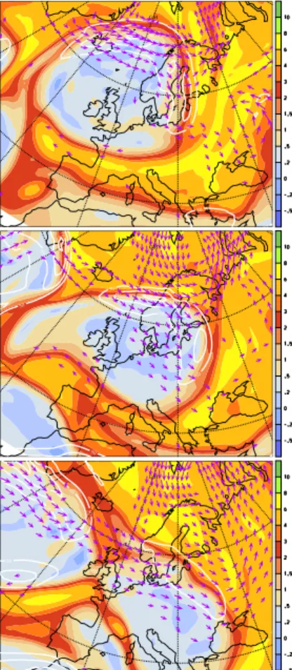
The meteorological situation leading to the mountain wave PSCs on 25–27 January over Scandinavia was discussed byD ¨ornbrack et al.(2002). Figure 1 shows the po-tential vorticity (PV) field on the 345 K isentropic surface, wind speed in the upper

5

troposphere (250 hPa) and wind vectors in the lower troposphere (900 hPa) for 25– 27 January 2000. The isentropic PV charts are well suited, for instance, to identify large-scale upper-tropospheric anticyclones (characterized by PV values < 2 pvu) and jet-stream regions (characterized by strong horizontal PV gradients). In agreement with Doernbrack et al. we note for 25 January the existence of an extreme upper-level

10

anticyclone over the UK, Iceland and Norway with strong low-level winds towards north-ern Norway and a northerly upper tropospheric jet over Scandinavia. In the course of the 3 days the anticyclone shifts southward and on 26 January a very strong jet is directly over central Scandinavia. The jet is almost parallel to strong near surface west-erlies, which provides very favourable conditions for excitation and vertical propagation

15

of mountain waves. On 27 January the anticyclone shifted further south, leaving rela-tively weak low- and upper-level winds over Scandinavia, except for the southernmost part with upper-level wind speeds ∼ 50 m/s.

3.2. PSC measurement

In this study lidar data is used from the NASA LaRC Aerosol Lidar (a piggy-back

instru-20

ment to the NASA GSFC AROTEL lidar) on board the NASA DC-8 aircraft (532 nm, 1064 nm) and the DLR OLEX lidar system on board the Falcon aircraft (354 nm, 532 nm, 1064 nm) (Flentje et al., 1999). Both systems measure total backscatter at all wavelengths and depolarization at 532 nm, which allows discrimination of spher-ical (STS) and aspherspher-ical (e.g. NAT and ice) particles. In addition, we will refer to the

25

ACPD

Full Screen / Esc

Print Version Interactive Discussion

c

EGU 2003

in-situ measurements on board the stratospheric research aircraft ER-2 on 27 January (Northway et al.,2002). Table 1 provides an overview of the platforms in operation on 25-27 January and from the data used in this study. The data is analyzed in Sect.4. 3.3. Analysis of lidar data

A lidar system emits a laser pulse and measures the backscatter from aerosols and air

5

molecules as a function of time. The backscatter ratio BSR is defined as

BSR= 1 + β

aerosol

βai r , (4)

where βaerosol is the backscatter coefficient of aerosol and βai r is the backscatter coefficient of air molecules (Rayleigh-scattering). The lidar system measures the total backscatter coefficient βtotal = βaerosol + βai r, and in order to obtain the backscatter

10

ratio, the backscatter coefficient βai r has to be calculated as a function of air density. The depolarization of the scattered laser pulse yields information about the shape of the scatterer. The aerosol depolarization is defined as:

δaerosol = β aerosol ⊥ βaerosol k (5)

where βaerosol_⊥ is the perpendicular aerosol backscatter coefficient and β_kaerosol is the

15

parallel aerosol backscatter coefficient. The color ratio is defined as the ratio of the aerosol backscattering coefficient at two wavelengths λ₁, λ₂with λ₁< λ₂:

CR(λ₁/λ₂)= βaerosol_λ 1 βaerosol_λ 2 (6)

The color ratio is very sensitive to the size of the scatterers, but independent of the number of scatterers. We will use the following notation: the backscatter ratio at

ACPD

Full Screen / Esc

Print Version Interactive Discussion

c

EGU 2003

1064nm ≡ BSR(1064), the color ratio βaerosol₅₃₂ /β₁₀₆₄aerosol≡ CR(532/1064), and the aerosol depolarization at 532nm ≡ δaer(532).

Based on long term lidar observations over Ny Alesund, Spitsbergen (78.9◦N, 11.9◦E) and T-Matrix calculations, Biele et al. (2001) presented a classification of li-dar data. They classify PSCs into the following types: type 1a (aspherical particles,

5

most likely NAT, low particle number densities n ≈ 10−2cm−3), type 1a-enh (aspher-ical particles, most likely NAT, high particle number densities n _{& 0.1 cm}−3), type 1b (ternary HNO₃/H₂SO₄/H₂O aerosol droplets (STS), n ≈ 10 cm−3), type mix (spheri-cal and aspheri(spheri-cal particles, likely NAT and STS particles mixed externally and not in thermodynamic equilibrium) and type 2 (ice particles, n=1-10 cm−3). We will use this

10

classification as a reference in our lidar data interpretation.

The backscatter of aspherical particles may be calculated using the T-Matrix method (Mishchenko,1991) (with spheroids of aspect ratio 0.5-1.5 as proxies for ice and NAT particles). The index of refraction is 1.31 for ice and 1.48 for NAT (Middlebrook et al.,

1994;Toon et al.,1994), that of STS obtained fromKrieger et al.(2000).

15

3.4. Microphysical modeling

A microphysical box model is used to calculate the evolution of the aerosol along a trajectory. The thermodynamics governing the condensation/evaporation kinetics of water and nitric acid by the aqueous sulfuric acid aerosol is calculated from an ion-interaction model (Pitzer,1991;Luo et al.,1995;Meilinger et al.,1995). The aerosol

20

size distribution is assumed to be log-normal with an initial mode radius of 0.06 µm and a mode width of 1.6 at T = 210 K. All calculations were performed with n = 13 cm−3 background aerosol particles, the sensitvity of the model results on background aerosol number density being small. The size distribution is modeled using 26 size bins for the liquid aerosol. Homogeneous ice nuleation in STS droplets is calculated from the

25

nucleation rates by Koop et al. (2000), and the ice vapor pressure is calculated in accordance with Marti and Mauersberger (1993). NAT nucleation on exposed ice

ACPD

Full Screen / Esc

Print Version Interactive Discussion

c

EGU 2003

surfaces is calculated in accordance withLuo et al.(2002), and the NAT vapor pressure is taken from Hanson and Mauersberger (1988). For each timestep, the number of nucleating ice and NAT particles is calculated for each size bin and transferred to new bins of their own. Upon evaporation of ice and NAT particles, the resulting droplets return into their original size bin.

5

The water mixing ratio in the Arctic stratosphere is taken from a linear interpolation of measured water mixing ratios on 27 January 2000 with a mixing ratio χ_H2O= 4.2 ppmv at 400 K and χ_H2O = 6.3 ppmv at 600 K (Schiller et al., 2002). In agreement with Arctic mid-winter measurements (Kleinb ¨ohl et al.,2003), an HNO₃profile with constant volume mixing ratio of 7.5 ppmv is used (altitude-dependent deviations in the order of

10

30 % may be expected in a real profile, but do not significantly alter model results). 3.5. Mesoscale modeling

Mesoscale numerical modeling studies (that include validation with observations) of gravity waves over Scandinavia that propagate into the stratosphere and lead to wave-induced PSCs were performed previously by D ¨ornbrack et al. (1999, 2001).

Fur-15

thermore, D ¨ornbrack et al. (2002) modeled 25-27 January 2000 episode with the mesoscale MM5 model. Here we calculated a series of mesoscale simulations with the High Resolution Model (HRM) (Majewski et al.,1991). A former version of this limited-area model was used operationally by the German and Swiss Weather Services until early 2001 and is widely used in the hindcast mode for regional climate simulations (e.g.

20

L ¨uthi et al.(1996)). The model integrates the set of primitive equations in the hydro-static limit. The initial and boundary conditions are taken from ECMWF analyses, and a radiative upper boundary condition prevents wave reflection. We use a dry physics ver-sion of the model without radiation and a horizontal resolution of 0.125◦(corresponding to ∼14 km) and 60 vertical levels up to 4 hPa (regularly spaced in log p). Further details

25

of the model setup can be found in Buss et al. (A gravity wave induced ice cloud over Greenland: Model validation and investigation of dynamical mechanisms, manuscript in preparation). Sensitivity studies showed that the simulation of the gravity wave and

ACPD

Full Screen / Esc

Print Version Interactive Discussion

c

EGU 2003

the associated temperature fields is sensitive to horizontal and vertical resolution and the initialization time, but insensitive to the height of the uppermost model level as well as inclusion of radiatation and moisture. For the simulations presented here, the orog-raphy was low-pass filtered with a conservative diffusion operator in order to eliminate the grid-scale components of the gravity wave. The simulations were started every 24

5

hours for integration periods of 36 hours, and the simulation steps 12-36 hours were used for the trajectory calculations.

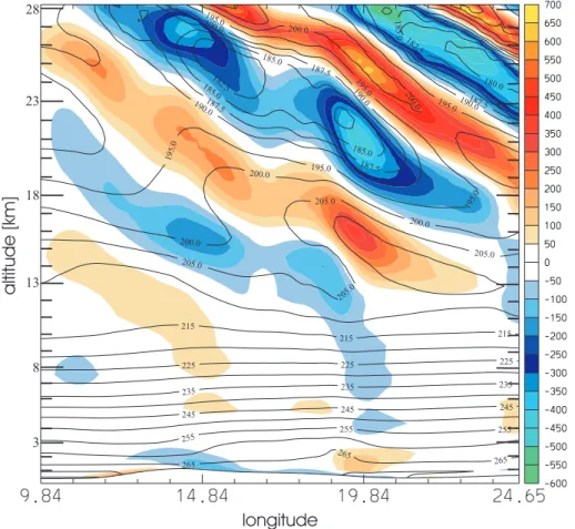
Figure2shows a vertical cross-section of the HRM simulation at 15:00 UTC, 26 Jan-uary. The propagating gravity wave becomes evident from the tilted bands of hori-zontal divergence and convergence whose amplitude increases with height. The

su-10

perimposed temperature field reveals two regions with temperatures below 185 K at 21–27 km altitude, in agreement with the location of PSCs (data shown below).

4. Classification of lidar data

Figure 3 shows an overview of the lidar measurements on 25-27 January. The lidar data was classified with the classification ofBiele et al.(2001) and shows PSCs over

15

Scandinavia on all 3 successive days. Figure4 shows the flight path of the selected lidar data segments, and Fig. 5 shows the results of the classification of these data segments according toBiele et al.(2001).

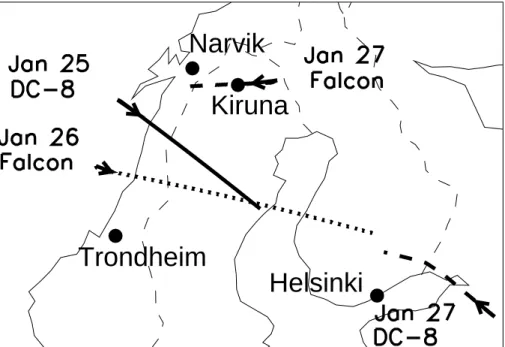
4.1. 25 January 2000

The DC-8 crossed the Scandinavian mountain ridge three times, and on each crossing

20

PSCs were observed, consisting of ice, STS, and likely NAT (see Fig.3). The LaRC lidar measurement between 15:03 UTC and 15:38 UTC (Figs.3and5a) are represen-tative for all lidar observations over Scandinavia on this day. The classification shows a large ice cloud over the Scandinavian mountain ridge, followed downstream by a type ‘mix’ cloud and finally a type 1a-enh PSC. This sequence of PSC type has been

ACPD

Full Screen / Esc

Print Version Interactive Discussion

c

EGU 2003

observed before [eg. Carslaw et al.(1998a);Wirth et al.(1999)] and is interpreted as follows. As the air approaches the mountain ridge, it is rapidly lifted and adiabatically cooled. When temperatures reach the necessary supercooling of ∼ 3 K, ice nuleation begins, leading to ice PSCs with high particle number densities due to the high cool-ing rates (∼ 30 K/h). Very rapid coolcool-ing also prevents the background aerosol to take

5

up HNO₃ before ice nucleation sets in, and the liquid aerosol droplets are initially out of thermodynamic equilibrium with the gas phase. Only during the evolutin of the ice cloud, the liquid takes up HNO₃ and depletes the gas phase. Behind the ridge the air sinks back to its original altitude, the temperature rises and the ice particles evap-orate. Depending on temperature, also the liquid ternary solution droplets evaporate

10

HNO₃and develop back to binary H₂SO₄/H₂O droplets. Eventually, the NAT particles evaporate when the temperature rises above the existence temperature T_NAT, which is about 8 K above T_ice (Hanson and Mauersberger,1988). Zondlo et al.(2000) provide a comprehensive overview over these processes.

Based on the LaRC lidar data, Hu et al.(2002) estimated ice particle number

den-15

sities in this PSC n_ice = 2 − 5 cm−3 with a mode radius r = 1.2 − 2 µm. NAT par-ticle number densities were estimated as n_NAT = 0.1 − 0.5 cm−3 with a mode radius

r = 0.4 − 1 µm, in general agreement with our analysis (not shown). Balloon-borne

in-situ measurements on this day at 20:30–22:30 UTC (see Fig.3) show the presence of STS and NAT particles downwind of the Scandinavian mountain ridge at altitudes

22-20

23 km, with a NAT particle number density of n ≈ 0.1 cm−3and a radius r = 0.5 −1 µm (Voigt et al.,2000).

4.2. 26 January 2000

Lidar observations on board of the Falcon aircraft show the presence of large ice PSCs over Scandinavia and patches of STS and type 1a-enh PSCs over the Atlantic ocean.

25

Downstream of the large ice cloud over Scandinavia (see Fig. 5b, at 200 - 600 km, and Fig.3) the Falcon observed a second ice PSC over Finland (see Fig.5b, at 750-850 km, and Fig.3). This rather unique observation of 2 large successive PSCs was

ACPD

Full Screen / Esc

Print Version Interactive Discussion

c

EGU 2003

chosen as a test case for the combined mesoscale/microphysical modeling approach (Sect. 5). The first ice PSC was also observed by ground-based FTIR, and based on the FTIR data, Hoepfner et al. (2001) estimated the average ice particle number densities n_ice = 2-5 cm−3, with a corresponding particle radius r = 2 − 1 µm, in general agreement with the analysis presented in Sect.5. Directly downstream of the first ice

5

PSC, following a small region of type “mix”, only a tiny margin of the PSC is identified as type 1a/1a-enh (see Fig.5b, at 300-650 km and 22-26 km alt.). A few isolated NAT “streaks” leave the lower part of the first ice cloud (see Fig.5b at ∼ 700 km). The PSC upstream of the first ice cloud (see Fig.5b, at 0-200 km, altitude ≈ 22 km) is classified as 1a-enh/mix/STS and is part of several stratified PSC patches observed at ≈ 22 km

10

altitude over the Atlantic (see Fig.3).

The second ice cloud shows a clearer type 1a-enh signal downstream. Unfortu-nately, the aircraft turned northward (and hence the subsequent flight leg is not quasi-Lagrangian) just when the type 1a-enh signal appears (see right edge of Fig.5b). The classification of STS below the second ice cloud indicates that NAT particles

(originat-15

ing from the first ice cloud), if present at all, must be small (r < 0.5 µm) and in very low number densities n_NAT ≈ 0.01 cm−3, such that the liquid droplets dominate the lidar backscatter.

4.3. 27 January 2000

On 27 January PSCs were sparse compared to the two preceding days. At 13:45 UTC

20

the Falcon observed a small (≈ 30 km in wind direction) ice PSC near Kiruna, about 50 km downstream of Kebnekaise, the highest peak in northern Scandinavia (18◦33’E/ 67◦53’N, elevation 2111 m). Downstream of and just below the ice PSC there is STS (see Figs.3and5c). The small geographical dimensions of the cloud indicates that in general temperatures were above the ice nucleation temperature, but single mountains

25

such as Kebnekaise may generate gravity waves of small horizontal dimensions and thus localized cooling.

ACPD

Full Screen / Esc

Print Version Interactive Discussion

c

EGU 2003

Helsinki/St.Petersburg (13:00–13:15 UTC, Figs. 3 and 5d). On the subsequent crossing of the mountain ridge, only STS was observed. The cloud near Helsinki classifies as type 1a-enh, type 1a and a small section as type 1b (STS). A hypothesis for the genesis of this NAT cloud will be presented in Sect.6.

In addition to the lidar data, in-situ measurements on board the NASA ER-2

strato-5

spheric research aircraft are available for this day. The ER-2 left Kiruna at ∼ 09:00 UTC and headed south over Finland towards Russia, from where it returned to Kiruna. Dur-ing the entire flight, the NO_y instrument found particulate matter at two positions only: on the outbound flight at ∼ 10:00 UTC, 27.83◦E/61.44◦N, and on the incoming flight at ∼ 13:15 UTC, 29.45◦E/59.9◦N. The two locations are in agreement with the lidar

ob-10

servation of the type 1a-enh PSC discussed above. Based on the NO_y data,Northway

et al. (2002) estimated a particle radius r ≈ 3 µm (outgoing flight leg) and r ≈ 4 µm (incoming flight leg) in low number densities n_NAT ≈ 3 × 10−4cm−3. T-Matrix calcula-tions for NAT particles of these sizes and number densities yield a backscatter ratio BSR(1064)_{. 1.25, which is far from the observed values BSR(1064) ≈ 3-15. The}

ob-15

served color ratio CR(532/1064) ≈ 1.1-3 of the lidar observation indicates that the cloud mainly consists of smaller particles (from T-Matrix calculations we estimate r ≈ 0.8 µm,

n_NAT ≈ 0.3 cm−3, corresponding to ∼ 3 ppmv HNO₃in the solid phase). This discrep-ancy between in-situ NO_y and lidar data may be resolved by the fact that the altitude of the ER-2 measurement (∼20 km) is at the extreme bottom of the PSC observed

20

by the lidar (see Fig. 5d). It can be speculated whether these larger particles at the cloud bottom result from sedimentation processes as proposed byFueglistaler et al.

(2002a); Dhaniyala et al. (2002). In addition, the NAT number densities at the edges of the cloud may be smaller due to less favorable nucleation conditions at cloud forma-tion time. Both processes can lead to the observed low number density. In sum we

25

may conclude that this cloud consists of NAT particles with r _{. 4 µm, most likely with}

r ≈ 0.8 µm and nNAT ≈ 0.3 cm −3

ACPD

Full Screen / Esc

Print Version Interactive Discussion

c

EGU 2003

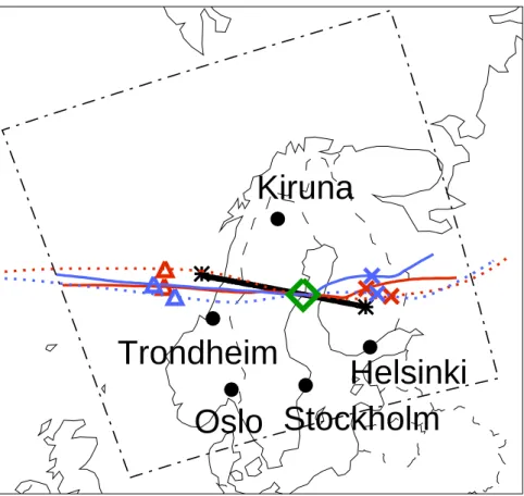
5. Detailed PSC modeling, 26 January 2000

A comprehensive microphysical box model (Luo et al.,2002) was used with trajecto-ries from NWP models. Forward and backward trajectotrajecto-ries were calculated starting at 20.37◦E/63.75◦N, 15:00 UTC between 400 K and 650 K potential temperature in in-crements of 2 K (corresponding to a vertical resolution ∼ 100 m, yielding a total of 126

5

trajectories), from both ECMWF analysis data and the HRM simulation. Figure6shows the flight path of the Falcon on 26 January (flight leg 3, black), ECMWF and HRM tra-jectories at 500 K (red) and 600 K (blue) and the trajectory starting position (green). The figure shows that the flight path is quasi-Lagrangian (i.e. parallel to the wind di-rection) and consequently the microphysical calculations along these trajectories can

10

be directly compared to the observations. Minor deviations between observations and calculated simulations should not come as a surprise, since flight path and trajecto-ries are not perfectly aligned, and the mountain wave cannot be considered as strictly stationary.

The simulated backscatter ratio BSR(1064) based on the results of the

microphys-15

ical calculations along the trajectories is shown in Fig.7 together with the measured backscatter ratio BSR(1064). This allows a direct comparison of simulations and mea-surements, while the underlying microphyiscal results, such as particle types and num-ber densities, are shown later (see Fig.9). Model results along trajectories are plotted in the geometry of the flight path (positions are resampled to equal distance from the

20

reference position where flight path and all trajectories intersect).

A comparison of the HRM-based PSC simulation (Fig.7b) with the measured lidar signal (Fig. 7a) shows that the simulation is in good agreement with the measure-ment. In particular, the shape of first ice cloud over Scandinavia fits the observation very well, and hence corroborates the HRM mesoscale simulation in combination with

25

the modeling of the ice nucleation. Also the second ice cloud is in general agree-ment with measureagree-ments, although its shape shows a tilt westward with height which is too strong compared to the measurement. Measured and simulated lidar

backscat-ACPD

Full Screen / Esc

Print Version Interactive Discussion

c

EGU 2003

ter ratios agree well and deviations are on average less than 25%. We conclude that the mesoscale/microphysical model simulation correctly reproduces the cloud micro-physics, in particular the particle types, number densities and sizes. It is emphasized again at this point that the simulation uses the meteorological parameters temperature and pressure from the HRM simulation without any modification, and that the

micro-5

physical box model calculates the nucleation of ice and NAT particles from nucleation rates rather than from prescribed values as in previous studies.

Upon closer inspection of measurement and simulation we note again the wrong tilt of the second ice cloud. A part of this tilt is an effect of the deviation between flight path and trajectories, however it is also apparent in the temperature field of the HRM

10

simulation. This tilt is also observed in the main ice cloud, where it causes trajectories to descend too soon compared to the measurement (i.e. ice particles evaporate too soon in the simulation, compare the ice regions with BSR(1064) > 100 at 24-25 km altitude in the measurement and simulation, Figs.7a,b). Further we note that the HRM-based simulation cannot reproduce the small scale waves (with wavelength_{. 20 km}

15

and amplitude _{. 5 K) superimposed on the dominant wave number observed in the} lidar data. It is clear that the mesoscale model with a spatial resolution of ∼ 15 km cannot resolve these waves. Calculations with a manually modified trajectory with these small scale waves superimposed on the HRM trajectory show that these waves can affect the microphysical properties quantitatively, but do not change the qualitative

20

properties of the cloud (calculations shown in the Appendix).

The simulation cannot reproduce the small PSC at 22 km altitude upstream of the first ice cloud, in Sect.4.2identified as STS and NAT, due to two reasons. Firstly, the microphysical model requires ice particles to initiate NAT nucleation, but the HRM sim-ulation temperatures do not reach the ice nucleation temperature upstream of

Scandi-25

navia. Secondly, the HRM backtrajectories are slightly further south than the flight path for this section over the Atlantic (see Fig.6). As will be shown later, a trough of air cold enough to form STS is present in the simulation at the location where the upstream PSC was observed, but its southern edge is just missed by the HRM trajectories.

ACPD

Full Screen / Esc

Print Version Interactive Discussion

c

EGU 2003

In contrast to the HRM-based simulation, the ECMWF-based simulation (Fig. 7c) fails to produce both ice clouds. ECMWF analysis temperatures also reach the ice frost point (see Fig.8a), but not the required supercooling for ice nucleation. An additional cooling of 1-2 K would lead to an ice PSC in a narrow altitude range around 510 K (not shown). In the ECMWF-based simulation the STS cloud upstream of the large

5

ice cloud is present, since ECMWF trajectories around the 500 K isentrope are further north (see Fig.6) than the HRM trajectories. Again, trajectories do not reach the ice nucleation temperature further upstream, and consequently the microphysical model fails to produce the observed NAT particles. A hypothesis on the origin of these NAT clouds is beyond the scope of this paper, but we note that these clouds might be a

10

challenge to test hypotheses on NAT nucleation.

Figure8shows an overview of the minimum temperatures and the calculated maxi-mum NAT saturation ratios in the presence of ice (S_NAT) along the trajectories used for this simulation. As expected from the lower spatial resolution, ECMWF analysis un-derestimates orographically induced temperature deviations from synoptic scale

tem-15

peratures. In addition, the underestimation of the wave amplitude yields NAT super-saturations considerably lower than the HRM-based trajectories. The latter yield very high NAT supersaturations of S_{NAT& 200, in agreement with the high supersaturations} found in manually constructed trajectories byLuo et al.(2002).

Figure 9a shows the maximum cooling rates found in the HRM trajectories and

20

ECMWF trajectories. The latter cannot reproduce the strong cooling rates found in mountain gravity waves and remain below 10 K/h. In contrast, the HRM trajectories show maximum cooling rates of 30–50 K/h, in accordance with manually constructed trajectories (Luo et al., 2002). The maximum cooling rates largely control the STS aerosol. With high cooling rates_{& 20 K/h the H2}O/HNO₃ uptake of the STS droplets

25

cannot keep pace with the decrease in vapor pressure, and the STS aerosol is out of equilibrium with the surrounding gas phase, resulting in extremely high NAT supersat-urations with respect to ice as shown in Fig.8b.

nu-ACPD

Full Screen / Esc

Print Version Interactive Discussion

c

EGU 2003

cleation, which controls the resulting ice particle number density. The largest droplets are to freeze first (due to their volume) and begin to deplete the gas phase. As a result, the ice saturation ratio (S_ice = p_part/p_vapor) decreases. When the saturation ratio falls below the supersaturation required for ice nucleation, further ice nucleation is inhib-ited. At high cooling rates_{& 15 K/h the decrease in partial pressure is compensated or}

5

even overcompensated by a decrease in vapor pressure, such that all droplets freeze (we will refer to this as 100% ice activation). The majority of cooling rates at onset of nucleation in the HRM trajectories is in the range 10–25 K/h. Consequently, most tra-jectories show ∼ 100% ice activation, despite the fact that nucleation begins at cooling rates significantly lower than the maximum values along the trajectories. In most cases,

10

the cooling rate further decreases during the next 3 min after onset of nucleation, but still remains too high in most cases to restrict resulting ice particle number density. The 3 min timeframe is motivated by the priod of continuous nucleation, which ranges from a few tens of seconds (rapid cooling) to a few minutes (slow cooling).

Figure10shows a summary of ice and NAT particle number densities in the

simula-15

tion. As expected from the cooling rates of the trajectories, the simulation yields almost 100% ice activation (n_ice ≈ 10 cm−3) at all altitudes where ice nucleation occurs. This is different for NAT nucleation on ice. The generally lower cooling rates at altitudes of 500–550 K (see Fig. 9b) allow the liquid aerosol to grow to larger sizes, and super-saturations with respect to NAT remain lower than at higher altitudes. Consequently,

20

the NAT nucleation rate calculated according toLuo et al.(2002) is lower, resulting in

n_NAT ≈ 0.1 − 0.5 cm−3. At higher altitudes the simulations yield NAT number densities of n_NAT ≈ 2 − 8 cm−3.

In order to quantify the accuracy of the modeled NAT and ice number densities, a detailed analysis of the lidar observations has been performed and is shown in the

Ap-25

pendix. The basic conclusion is that the mesoscale/microphysical model yields results in general agreement with measurements, and that the temperatures and cooling rates of mesoscale models such as HRM suffice to model mountain wave PSCs.

ACPD

Full Screen / Esc

Print Version Interactive Discussion

c

EGU 2003

6. Modeling of PSC evolution, 25–27 January 2000

In the previous section it was shown that the combined mesoscale/microphysical mod-eling approach yields results in good agreement with observations. Now we will use this approach to model the 3-dimensional evolution of the PSCs on 25–27 January 2000. Similar to the previous simulation we calculated trajectories from the HRM

sim-5

ulation and used these trajectories as input for the microphysical boxmodel. For this simulation we calculated for each day 200 trajectories on two potential temperature lev-els, started along a line from 12◦E/59◦N to 28◦E/72◦N. Based on the altitude level of PSC observations in the lidar data, simulations for 500 and 550 K potential temperature are shown for 25 and 26 January in Figs.11and12. On 27 January the simulations for

10

490 and 500 K are shown. Based on the times of the lidar observations, trajectories were started 15:00 UTC for 25 and 26 January and 11:00 UTC for 27 January.

6.1. 25 January 2000

The simulations show STS, NAT and ice clouds both on the 500 K and 550 K level. From a comparison with measurements (see Fig. 3), it is apparent that the

simula-15

tion overestimates temperatures over northern Scandinavia by 1–3 K. The simulations show mainly STS in this region, whereas the measurements show a large ice PSC near Kiruna. The ice PSCs over central Scandianvia are correctly modeled (indicated in Fig.11by BSR(1064) > 50, see also Fig.12). An inspection of NAT number densities in the trajectories that fit best the track of the balloon-borne experiment (near Kiruna)

20

presented byVoigt et al. (2000) shows NAT number densities n_NAT ≈ 0.1 cm−3. This value is in good agreement with the measured n_NAT ≈ 0.1 cm−3 (Voigt et al., 2000). Over central Scandinavia, the simulation yields n_NAT= 0.2-3 cm−3 (see Fig.12), which is also in good agreement with the results of the analysis of lidar data by Hu et al.

(2002), who estimated for this region n_NAT = 0.1 − 0.5 cm−3.

ACPD

Full Screen / Esc

Print Version Interactive Discussion

c

EGU 2003

6.2. 26 January

The simulation of the Falcon measurement (see Sect.4.2) showed that the simulation and the measurements of this day are in almost prefect agreement with respect to PSC type and spatial dimensions. This is also apparent in these simulations on the 500 K and 550 K isentropes. These simulations furthermore show that NAT clouds

down-5

stream of the northern part of the first ice PSC prevail downstream until the trajectories leave the domain of the simulation (the region with BSR(1064) ≈ 15, identification of NAT in the simulation after inspection of the data of the microphysical simulation, Fig.12). The presence of a region where the NAT PSC evaporates ∼ 200 km down-stream of the ice cloud highlights again the fact that, depending on the temperature

10

history, NAT can also be absent downstream of an ice PSC. It was earlier mentioned that the simulation of the vertical cross-section of 26 January based on HRM data does not show the observed STS cloud upstream of the ice PSC. The simulations shown here support the explanation suggested earlier that the slight displacement of the flight path and the trajectories is responsible for the disagreement. The horizontal

15

simulation reveals a pool of cold air located over the Atlantic, giving rise to STS clouds (BSR(1064) ≈ 3, identification of STS after inspection of the data of the microphysi-cal simulation). The simulated STS cloud is in agreement with observed STS clouds (see Fig.3), and ceases to exist at approximately the latitude where the Falcon aircraft turned eastward.

20

6.3. 27 January

The simulation of this day misses the small ice PSC ∼ 50 km downstream of Keb-nekaise (18◦33’E/67◦53’N, elevation 2111 m), but correctly predicts the observed STS cloud at the same location. Apparently, the HRM model slightly overestimates tem-peratures in this region. Considering the limited horizontal resolution (∼ 15 km) of the

25

HRM model and the smoothed orography, it seems plausible that the model underes-timates gravity waves caused by high, but horizontally small orographic features such

ACPD

Full Screen / Esc

Print Version Interactive Discussion

c

EGU 2003

as Kebnekaise.

The presence of an STS cloud over central Scandinavia in the simulation (with BSR(1064)_{. 10) is confirmed by the LaRC measurements on board the DC-8 (see} Fig. 3). The simulation does not show the observed NAT PSC near Helsinki/St. Pe-tersburg (see Figs. 3 and 5d), but holds a plausible explanation for the cloud. The

5

simulation shows the presence of a small ice cloud over southern Scandinavia (near Oslo), which gives rise to a NAT cloud downstream (the small line in the horizontal sim-ulation with BSR(1064)= 2−10, identification of NAT after inspection of the data of the microphysical simulation, Fig.12). In the simulation, temperatures further downstream are slightly too high such that the NAT particles evaporate shortly before the air

trajec-10

tory intersects with the flight path. We have refrained from lowering the temperatures by ∼ 1 K which would be required to produce a ‘match’ with the observed type 1a-enh PSC, to remain in accordance with all other simulations where all meteorological pa-rameters of the NWP models remained unaltered. An inspection of the data of the microphysical simulation (see Fig. 12) shows a number density of the ice cloud near

15

Oslo n_ice = 0.01 − 8 cm−3 (i.e. also very slow cooling rates at the onset of nucleation). The simulated NAT cloud downstream shows n_NAT = 0.01 − 2 cm−3(i.e. a large range of number densities), which is in agreement with our earlier calculations based on the measured lidar data, which concluded n_NAT ≈ 0.3 cm−3and r ≈ 0.8 µm.

7. Conclusions

20

We presented a detailed modeling study of orographically induced gravity wave PSCs over Scandinavia on 25–27 January 2000 by means of a combined mesoscale/microphysical model. Extensive observation of this PSC event during the second phase of the SOLVE/THESEO-2000 Arctic campaign provides an excellent data set of ground-based, balloon-borne and aircraft-borne in-situ and remote sensing

25

measurements. We analyzed lidar data of the DLR OLEX system on board the Falcon aircraft and of the NASA LaRC system on board the DC-8. In addition, we compared

ACPD

Full Screen / Esc

Print Version Interactive Discussion

c

EGU 2003

the model results with data of the NO_yinstrument on board the NASA ER-2 (Northway

et al.,2002) and balloon-borne mass spectrometer data (Voigt et al.,2000).

The model simulations use trajectory calculations based on mesoscale simulations with the High Resolution Model (HRM) as input for our microphysical box model. All microphysical calculations use the meteorological information of the trajectories without

5

modifications (i.e. without “tuning” of the temperature). We calculate a lidar signal from the microphysical simulation with T-Matrix calculations for aspherical particles and Mie calculations for liquid particles. The comparison of simulations and measurements shows:

(a) The mesoscale HRM simulations of orographically induced gravity waves over

10

Scandinavia are in good agreement with lidar observations. As a general tendency, the wave amplitude appears to be slightly underestimated rather than overestimated, such that the simulations do not always yield ice when observations indicate the pres-ence of ice. However, in general the mesoscale simulation captures minimum tempera-tures and cooling rates well. Sensitivity studies show that the results of the mesoscale

15

modeling are robust, i.e. that for different model setups the results do not critically differ. We conclude from this study that the mesoscale modeling is sufficiently reliable to model the microphysics of mountain wave ice PSCs over Scandinavia, even though it still misses very small ice clouds which may be caused by orographic features that are either not present in the model orography or cause gravity waves which cannot be

20

resolved even with a horizontal resolution of ∼ 15 km.

Simulations with ECMWF analysis data show that the model, as a consequence of its synoptic scope and coarse resolution, severely underestimates lowest temperatures and cooling rates. Consequently, ECMWF data (and data of other NWP models with similar spatial resolution) are only suited for the study of liquid PSCs on a synoptic

25

scale.

(b) The simulations show that in mountain wave PSC events the ice PSC

observa-tions are in agreement with simulaobserva-tions assuming homogeneous ice nucleation and using the parametrization ofKoop et al.(2000). The accuracy of the mesoscale

trajec-ACPD

Full Screen / Esc

Print Version Interactive Discussion

c

EGU 2003

tory calculations is not sufficient to resolve details of the ice PSCs, but on a statistical basis the simulations yielded both ice number densities and particle sizes within the range of observations. We estimate the accuracy of the modeled particle number den-sities within a factor 2 for ice particles. A more precise estimation of the accuracy is not (yet) possible due to the uncertainties in the interpretation of the (lidar) data.

5

(c) This modeling study assumes NAT nucleation on ice according to the process

de-scribed byLuo et al.(2002). All observations of NAT in the region of interest could be explained with this process except patches of NAT clouds over the Atlantic, which we have not further analyzed in this study. This study supports the assumption that NAT forms in (mountain wave) ice PSCs, though it does not exclude other nucleation

mech-10

anisms. The accuracy of the modeled NAT number density is estimated to be within a factor 10, the uncertainty again largely caused by uncertainties in the interpretation of the measurements. The importance of combined in-situ and lidar measurements to finally overcome limitations in the lidar data retrieval cannot be overemphasized.

(d) If NAT nucleation on ice is of importance to the denitrification of the polar

strato-15

sphere (e.g. via sedimentation of NAT particles out of high number density NAT clouds as proposed by Fueglistaler et al., 2002a,b; Dhaniyala et al., 2002), then Chemical Transport Models (CTM) using synoptic scale temperature and wind fields miss a key element in the process of ozone destruction. Ice PSCs cannot be simulated realiably with synoptic scale temperature fields, and consequently the formation of NAT

parti-20

cles, their sedimentation and the resulting denitrification is not accurate.

In summary, this study shows that the combined mesoscale/microphysical modeling approach yields results in good agreement with observations and enables the inves-tiagation of the 3-dimensional structure of mountain wave PSCs. The results of this approach are the first of their kind and show a level of detail in the modeling and

com-25

parison with measurements not performed before. It is shown that the current under-standing of PSC microphysics and mesoscale dynamics modeling suffices to explain the key characteristics of mountain wave PSC events. However, the study also implies that currently available data do not suffice to draw new conclusions about the

micro-ACPD

Full Screen / Esc

Print Version Interactive Discussion

c

EGU 2003

physics of PSCs (despite the excellence of the SOLVE/THESEO-2000 campaign data). It is conceivable that future Arctic campaigns use not only meteorological forecasts, but also microphysical calculations based on mesoscale forecasts to guide mission planning. This approach could contribute to observations that allow to reject or prove suggested microphysical processes in PSCs, and hence to a significant improvement

5

of our understanding of PSC formation.

Appendix: Detailed lidar data retrieval 26 Jan 2000

Figure 13 shows the measured color ratio CR(532/1064), scatterplots of the data in the δaer(532)/BSR(1064) plane (Figs. 13b, c, d) together with color ratios calculated with the T-Matrix method for ice and NAT particles (Figs.13e, f; the particle shape is a

10

spheroid with aspect ratio 0.5 to 1.5).

Four regions of particular interest are indicated in Fig.13a. Regions “A” and “B” refer to two regions of the ice cloud with a distinct color ratio. Data of region “A” shows a higher color ratio and a tendency towards lower aerosol depolarization (see Fig.13b) compared to region “B” (note that the plotting in a scatterplot leads to an overplot of a

15

small fraction of data with high color ratio and high aerosol depolarization). Regions “C” and “D” cover areas of interest with respect to the occurrence of NAT particles. Data of these regions cannot be univocally identified in the scatterplot due to noise in the depolarization data at BSR(1064). 5 (probably caused by an iced window, H. Flenje, pers. comm.).

20

Ice particles

The observed difference in color ratio in the ice cloud between regions above ∼ 23 km (“A”) and below (“B”) indicates that the sizes of the ice particles in the two regions differ. Region “A” shows a high backscatter and a color ratio CR(532/1064) = 5 − 9. Based on the T-Matrix calculations shown in Fig. 13e, we estimate ice particle sizes

ACPD

Full Screen / Esc

Print Version Interactive Discussion

c

EGU 2003

r = 1 − 1.5 µm (with aspect ratio ∼ 0.9) in this region. In thermodynamic equilibrium

at T ≈ T_ice− 3 K a particle size of r ≤ 1.5µm requires n_ice ≥ 10 cm−3. This implies that basically the entire background aerosol froze, which in turn requires cooling rates

> 10 K/h at the onset of ice nucleation (based on sensitivity studies for different cooling

rates, calculated with the microphysical box model). The calculated ice number

densi-5

ties in the simulation in this region of n_ice = 10 − 12 cm−3(see Fig.10) agree well with these considerations based on the lidar data.

Region “B” shows a similar BSR(1064) as region “A”, but has a significantly lower color ratio CR(532/1064) < 1.5. An inspection of the T-Matrix calculations (see Fig. 13e) shows that the observations can be explained by ice particles of size

10

r _{& 1.8 µm and aspect ratio 0.9, with a corresponding particle number density} n_{ice . 5cm}−3. Calculations show that altitude-dependent variations in available wa-ter vapor affect ice particle sizes, but cannot be the only reason for the different color ratios of regions “A” and “B”. Rather, we consider a different particle shape of ice parti-cles in the two regions a likely cause. Figure13e shows that particles with aspect ratio

15

∼ 0.65 show moderate color ratios CR(532/1064) . 2 for practically all particle sizes. This is in accordance with the fact that a distinct peak in color ratio, as expected for growing ice particles with aspect ratio_{& 0.8, is not observed in region “B”. In principle,} also very slow cooling rates (_{. 2.5 K/h) could lead to the observed low color ratios,} even for particles with aspect ratio 0.85. Cooling rates_{. 2.5 K/h lead to nice . 1 cm}−3

20

ice particles, which follow a wide size distribution, such that the distinct peak in color ratio at r ≈ 1 µm diminishes. An estimation of cooling rates based on the lidar data of the STS cloud upstream of the ice cloud yields an average cooling rate ∼ 10 K/h (in agreement with the HRM simulation, Fig. 8b), which is considerably higher than the required 2.5 K/h. Even under the assumption of lower cooling rates at the begin

25

of nucleation, an aspect ratio ∼ 0.85 for ice particles appears unlikely. Minor varia-tions in the cooling rate of ±1 K/h (which can be safely expected for the stratosphere) inevitably lead to variations in particle number density that cause significantly higher than observed color ratios. Thus, we consider differing aspect ratios in region “A” and

ACPD

Full Screen / Esc

Print Version Interactive Discussion

c

EGU 2003

“B” the most likely hypothesis for the systematic difference in color ratio.

On the reason for a systematic difference in particle shapes of region “A” and “B” we can only speculate. As outlined above, cooling rates are lower upstream of region “B” (though still high enough to freeze most of the background aerosol). Consequently, the ice particles of region “B” nucleated in larger droplets and grew in an environment

5

closer to the thermodynamic equilibrium, which could favour crystal growth along the preferred axes, and hence a more prolate shape.

To conclude this discussion of the ice PSC, we note that the mesoscale HRM simu-lation cannot help to support or reject any of the hypotheses presented above. On the one hand, the HRM simulation underestimates the cooling rates upstream of region

10

“A”, as indicated by the presence of STS upstream of the ice region in the simulation in contrast to the observation (see Fig.7b). On the other hand, the mean cooling rates upstream of region “B” appear realistic from a comparison of the horizontal dimensions of the STS upstream of region “B”. Yet, the cooling rates at the location of ice nucle-ation is still too high (see Fig.9b) to severly reduce the number of freezing particles

15

(see Fig.10). The extreme sensitivity of ice nucleation rates on cooling rates would re-quire trajectories with an accuracy in cooling rates within ±0.5 K/h, which is far beyond from what current NWP models can deliver.

NAT particles

The lidar classification discussed in Sect. 4.2 shows a substantial fraction of pixels

20

directly downwind of the ice cloud (region “D”) classified as “NAT” or “mixed”, but the signal is noisy. Here we compare the signal in the two regions “C” and “D” (Figs.13c, d). Region “C” is clearly classified as STS, “mix” and a layer of NAT particles. The layer dominated by NAT shows a distinct color ratio CR(532/1064)= 1 − 2, whereas the other parts of region “C” show CR(532/1064)_{& 3.25. A comparison with T-Matrix}

25

calculations (Fig. 13f) shows that the observed signal (significant depolarization and color ratio CR(532/1064)= 1 − 2) is in agreement with NAT particles with r & 0.5µm. The observed backscatter ratio BSR(1064)= 5 − 30 indicates n_NAT = 0.5 − 3 cm−3NAT

ACPD

Full Screen / Esc

Print Version Interactive Discussion

c

EGU 2003

particles (with r = 0.5µm), with a corresponding HNO₃ mixing ratio 1–5 ppbv in the solid phase.

Region “D” shows similar aerosol depolarization as region “C”, but a lower backscat-ter ratio (BSR(1064) = 5 − 15) and color ratios CR(532/1064) = 1.5 − 3.25. This indicates that region ‘D’ contains NAT particles with a size r _{. 0.5µm and particle}

5

number densities of n = 0.5 − 10 cm−3, corresponding to < 3 ppbv HNO₃ in the solid phase. This analysis shows that n= 0.5 − 10 cm−3NAT particles may well be present downwind of the ice PSC, but the period of time where temperatures are too high for STS but still below T_NAT is too small to cause a clear 1a-enh classification.

Simulation results of a manually optimized trajectory

10

Figure 14 shows a detailed comparison of microphysical and optical parameters be-tween model calculations along the HRM 550 K trajectory and a manually modified trajectory (based on the 550 K HRM trajectory and lidar data interpretation; the white line in Fig. 7a shows the location of the trajectory in the geometry of the lidar data). The figure shows that much of the inconsistency between measured lidar signal and

15

HRM-based simulations can be explained by a few shortcomings in the HRM trajec-tory. In particular, the spatial wavelength of the main gravity wave over Scandinavia is underestimated in the HRM simulation, and temperatures of the manual trajectory remain longer below T_ice (see Fig.14a), and hence ice particles prevail.

The cooling rates of the manual trajectory were adjusted in the area where ice

nu-20

cleation occurs, such that the observed and modeled lidar backscatter agree. For this trajectory, n_ice≈ 10 cm−3yield an inferred lidar signal in best agreement with the obser-vations. The temperature variations due to the small scale waves (not resolved in the HRM simulation) lead to a variation of the simulated lidar backscatter in good agree-ment with the observed variation of BSR(1064) in the ice cloud. While the simulated

25

backscatter ratio at 1064 nm is in good agreement with observations (independently of aspect ratio), it is more difficult to correctly model CR(532/1064) and aerosol de-polarization. Figures14b/c show the observed and simulated color ratios and aerosol

ACPD

Full Screen / Esc

Print Version Interactive Discussion

c

EGU 2003

depolarizations. For the second ice cloud, which has a lidar signal similar to the ear-lier discussed region “B”, we used an ice particle aspect ratio 0.7, in accordance with our earlier considerations (all other calculations used an aspect ratio 0.85 for ice parti-cles). The calculation with aspect ratio 0.85 for ice particles is in good agreement with measured color ratios in the first ice cloud, but overestimates aerosol depolarization.

5

In contrast, the calculation with aspect ratio 0.7 for the second ice cloud is in good agreement with observed aerosol depolarization, but overestimates color ratios.

As a result of the rapid cooling, the model yields downwind of the first ice PSC (at ∼ 13–14:00 UTC) n_NAT ≈ 10 cm−3 NAT particles (i.e. on most ice particles a NAT parti-cle nuparti-cleated). Backscatter, color ratio and depolarization of the sections where NAT

10

particles prevail are in general agreement with the observations. Deviations may be explained by the fact that it is difficult to follow the air flow in the lidar image, and con-sequently the manual trajectory is not perfectly quasi-Lagrangian (note the increased scatter in the lidar data around 13:30–14:00 UTC). Downwind of the second PSC the simulation yields n_NAT= 5 − 10 cm−3NAT particles (again almost 100 % activation).

15

In summary, the manually modified trajectory improves the agreement between sim-ulation and measurement, but does not fundamentally change the results obtained with the HRM trajectories. The original HRM trajectory may not be able to resolve details, but yields particle number densities and sizes very similar (within a factor 2) to the man-ually optimized trajectory. From this detailed analysis we conclude that the combined

20

mesoscale/microphysical modeling approach yields results in general agreement with measurements, and that temperatures and cooling rates of mesoscale models such as HRM suffice to model mountain wave PSCs.

Acknowledgements. SF and SB have been supported through the EC-project THESEO-2000/EuroSOLVE (under contract BBW 99.0218-2, EVK2-CT-1999-00047) and through an

25

ETHZ-internal research project. BL has been supported through the EC-project MapScore. We thank D. L ¨uthi for his help with the setup of the HRM model. We thank A. D ¨ornbrack, C. Schiller, T. Deshler, and C. Voigt for fruitful discussions.

ACPD

Full Screen / Esc

Print Version Interactive Discussion

c

EGU 2003

References

Biele, J., Tsias, A., Luo, B. P., Carslaw, K. S., Neuber, R., Beyerle, G., and Peter, Th.: Nonequi-librium coexistence of solid and liquid particles in Arctic stratospheric clouds, J. Geophys. Res., 106, 22991–23007, 2001. 256,260,262,288,290

Browell, E. V., Butler, C. F., Ismail, S., Robinette, P. A., Carter, A. F., Higdon, N. S., Toon, O.

5

B., Schoeberl, M. R., and Tuck, A. F.: Airborne Lidar Observations In The Wintertime Arctic Stratosphere: Polar Stratospheric Clouds, Geophys. Res. Lett., 17, 385–388, 1990. 255

Carslaw, K. S., Luo, B. P., Clegg, S. L., Peter, Th., Brimblecombe, P., and Crutzen, P. J.: Strato-spheric aerosol growth and HNO₃gas phase depletion from coupled HNO₃and water uptake by liquid particles, Geophys. Res. Lett., 21, 2479–2482, 1994. 255

10

Carslaw, K. S., Wirth, M., Tsias, A., Luo, B. P., D ¨ornbrack, A., Leutbecher, M., Volkert, H., Renger, W., Bacmeister, J. T., and Peter, Th.: Particle microphysics and chemistry in re-motely observed mountain polar stratospheric clouds, J. Geophys. Res., 103, 5785–5796, 1998a. 256,257,263

Carslaw, K. S., Wirth, M., Tsias, A., Luo, B. P., D ¨ornbrack, A., Leutbecher, M., Volkert, H.,

15

Renger, W., Bacmeister, J. T., Reimer, E., and Peter, Th.: Increased stratospheric ozone depletion due to mountain-induced atmospheric waves, Nature, 391, 675–678, 1998b. 255

Dhaniyala, S., McKinney, K. A., and Wennberg, P. O.: Lee-wave clouds and denitrification of the polar stratosphere, Geophys. Res. Lett., 29, 9, 1322, doi:10.1029/2001GL013900, 2002.

265,274

20

D ¨ornbrack, A., Leutbecher, M., Kivi, R., and Kyr ¨o, E.: Mountain wave-induced record low strato-spheric temperatures above northern Scandinavia, Tellus, 51A, 951–963, 1999. 261

D ¨ornbrack, A., Leutbecher, M., Reichardt, J., Behrendt, A., M ¨uller, K.-P., and Baumgarten, G.: Relevance of mountain wave cooling for the formation of polar stratospheric clouds over Scandinavia: Mesoscale dynamics and observations for January 1997, J. Geophys. Res.,

25

106, 1569–1581, 2001. 261

Doernbrack, A., Birner, Th., Fix, A., Flentje, H., Meister, A., Schmid, H., Browell, E. V., Mahoney, M. J.: Evidence for inertia-gravity waves forming polar stratospheric clouds over Scandinavia, J. Geophys. Res., 7, D20, 8287, doi:10.1029/2001JD000452, 2002. 258,261

Fahey, D.W., Gao, R. S., Carslaw, K. S., Kettleborough, J., Popp, P. J., Northway, M. J., Holecek,

30

J. C., Ciciora, S. C., McLaughlin, R. J., Baumgardner, D. G., Gandrud, B., Wennberg, P. O., Dhaniyala, S., McKinney, K. A., Peter, Th., Salawitch, R. J., Bui, T. P., Elkins, J. W., Webster,