UNIVERSITÉ DE MONTRÉAL
COMPUTATION OF FREQUENCY DEPENDENT NETWORK EQUIVALENTS USING VECTOR FITTING, MATRIX PENCIL METHOD AND LOEWNER MATRIX
JESÚS MORALES RODRÍGUEZ DÉPARTEMENT DE GÉNIE ÉLECTRIQUE ÉCOLE POLYTECHNIQUE DE MONTRÉAL
THÈSE PRÉSENTÉE EN VUE DE L’OBTENTION DU DIPLÔME DE PHILOSOPHIAE DOCTOR
(GÉNIE ÉLECTRIQUE) MAI 2019
UNIVERSITÉ DE MONTRÉAL
ÉCOLE POLYTECHNIQUE DE MONTRÉAL
Cette thèse intitulée :
COMPUTATION OF FREQUENCY DEPENDENT NETWORK EQUIVALENTS USING VECTOR FITTING, MATRIX PENCIL METHOD AND LOEWNER MATRIX
présentée par : MORALES RODRÍGUEZ Jesús
en vue de l’obtention du diplôme de : Philosophiae Doctor a été dûment acceptée par le jury d’examen constitué de :
M. HOUSHANG Karimi, Ph. D., président
M. MAHSEREDJIAN Jean, Ph. D., membre et directeur de recherche M. KOÇAR Ilhan, Ph. D., membre et codirecteur de recherche
M. RAMIREZ Abner, Ph. D., membre et codirecteur de recherche M. SHESHYEKANI Keyhan, Ph. D., membre
DEDICATION
ACKNOWLEDGEMENTS
Firstly, I would like to thank professors Jean Mahseredjian and Ilhan Kocar for their trust since the first contact we had for coming to Polytechnique de Montréal, but also for the guidance and for sharing their expertise as researchers during my PhD studies.
Equally, I would like to express my enormous gratitude to professor Abner Ramírez, first, for encouraging me to come to Canada to pursue the PhD degree, and second, for his wise advices, not only as a professor but also as a friend.
Also, my sincere thanks to professor Keyhan Sheshyekani for his very valuable advices and guidance during my PhD.
I would like to specially thank the person who encourages me every day to achieve my personal goals, who has changed the way I understand life, and therefore, has been very important during this stage of my life, Gwendoline.
Also, many thanks to my family, my parents Jesus and Pilar, and my sisters Janine and Jessica, for the encouragement and for the unconditional support in both, good and difficult times.
Many thanks to my department colleagues, who are my friends at the same time, Miguel, Haoyan, Ming, Anton, Aramis, Reza, professor Akiro Ametani, Isabel, Masashi, Baki, Thomas, Nazak, Diane, David, Aboutaleb, Serigne, Louis, Willy and Edgar, for all the good moments we have spent together.
Finally, I would like to thank the chair partners: Polytechnique de Montréal, CNSRC, Hydro-Québec, Opal-RT, EDF and RTE for the financial support.
RÉSUMÉ
Cette thèse présente l’analyse des techniques existantes et des nouveaux développements pour le calcul d’équivalents de réseaux électriques (FDNEs en anglais). Les FDNEs sont des modèles rationnels d’ordre réduit de dispositifs ou de parties de réseaux, utilisés pour l’accélération des simulations de transitoires électromagnétiques. Un FDNE est calculé de façon à ce que sa réponse fréquentielle corresponde à celle du système original dans une bande de fréquences definie. Ce qui permet la réduction de l’ordre du modèle et par conséquent, la réduction du temps de calcul des simulations dans le domaine du temps.
Pour l’application de la technique FDNE, le système original et le modèle équivalent doivent être linéaires, causals et passifs. Ces caractéristiques sont étudiées en détail dans cette thèse, ainsi que la dérivation mathématique de la matrice Hamiltonienne et la matrice de singularité associée pour l’évaluation de la passivité des FDNEs.
Les FDNEs sont calculés à l’aide d’une technique d’ajustement de courbes. Ensuite, la passivité du modèle doit être évaluée, et, si des violations de passivité sont découvertes, une technique pour forcer la passivité du modèle doit être appliquée pour assurer la stabilité numérique du modèle. Dans la littérature, les techniques existantes pour l’ajustement de courbes et pour forcer la passivité des modèles rationnels sont nombreuses, donc, les plus matures ont été sélectionnées et étudiées. Les théories de ces techniques sont analysées et comparées avec des exemples numériques. À partir des résultats obtenus des ces études, la technique Vector Fitting (VF) est reconnue comme la plus précise. Cependant, les techniques Matrix Pencil Method (MPM) et Loewner Matrix (LM) sont reconnues comme des techniques utiles pour l’identification de l’ordre des modèles équivalents. Finalement, une nouvelle technique est proposée en combinant les techniques étudiées. La méthodologie proposée est plus efficace que les techniques étudiées appliquées de façon individuelle.
En ce qui concerne la passivité des modèles FDNE, un problème majeur avec les techniques qui forcent la passivité est identifié comme suit. Pour des FDNEs d’ordre élevé, ou des FDNEs dotés de nombreux ports de connexion, ou une combinaison des deux, les techniques étudiées, Fast Residue Perturbation (FRP), Hamiltonian Matrix Perturbation (HMP) et Semidefinite Programming (SDP) sont numériquement très coûteuses, et parfois incapables de trouver une solution. Donc, une nouvelle technique, nommée Pole-Selective Residue Perturbation (PSRP) est
proposée. Contrairement aux techniques traditionnelles, la technique PSRP calcule les perturbations de façon algébrique, permettant une meilleure performance numérique que les techniques FRP, HMP et SDP. En plus, la technique proposée permet de trouver des solutions aux problèmes pour lesquels les techniques traditionnelles échouent.
ABSTRACT
This thesis presents a thorough analysis of existing techniques and new developments for the calculation of Frequency-Dependent Network Equivalents (FDNEs). FDNEs consist of reduced-order rational models of devices or subnetworks aimed at acceleration of electromagnetic transient (EMT) simulations. A FDNE is calculated such that the frequency-response of the original model is matched for a finite frequency band, this allows the reduction of the model order and consequently, the reduction of computational burden in time-domain simulations.
For the application of the FDNE approach, both, the original and equivalent (FDNE) models are required to be linear, causal and passive. These modeling requirements are studied in detail in this thesis. Also, the mathematical derivation of the Hamiltonian matrix and associated singularity test matrix for the passivity assessment of rational models is reviewed.
The computation of FDNEs is achieved by applying a curve fitting approach to identify the system’s equivalent rational model. Then, the passivity of the model must be assessed, and, in case that passivity violations are revealed, a passivity enforcement technique must be applied to guarantee numerical stability of the model in transient simulations.
Since different techniques exist for both, rational modeling and passivity enforcement, the most relevant are chosen and further studied. The theories of these techniques are first revisited, then, the studied techniques are compared with numerical examples. From these numerical studies, the Vector Fitting (VF) technique is demonstrated to be the most accurate technique for rational modeling. However, the Matrix Pencil Method (MPM) and Loewner Matrix (LM) technique are shown to be useful methods for model order identification. Thus, a novel fitting technique, consisting of a combination of the above-mentioned techniques, is proposed. The new methodology is demonstrated to be more efficient than any of the involved techniques applied independently.
Regarding the passivity enforcement stage, a major issue is identified as follows. For high-order FDNE models, or FDNEs with many connection ports, or a combination of both, available passivity enforcement techniques, such as the Fast Residue Perturbation (FRP), Hamiltonian Matrix Perturbation (HMP) and Semidefinite Programming (SDP), are either computationally very expensive or unable to find a solution due to the large computational burden required. Then, a novel passivity enforcement technique named Pole-Selective Residue Perturbation (PSRP) is
proposed. Unlike the existing techniques, the PSRP method consists of algebraic calculations, instead of solving optimization problems as required by the traditional methods. This feature of the proposed technique allows improved computational performance compared to the FRP, HMP and SDP techniques. Additionally, the proposed method allows finding a solution to problems for which the traditional techniques fail.
TABLE OF CONTENTS
DEDICATION ... III ACKNOWLEDGEMENTS ... IV RÉSUMÉ ... V ABSTRACT ... VII TABLE OF CONTENTS ... IX LIST OF TABLES ... XIII LIST OF FIGURES ... XV LIST OF SYMBOLS AND ABBREVIATIONS ... XIX LIST OF APPENDICES ... XX CHAPTER 1 INTRODUCTION ... 1 1.1 Literature review ... 2 1.2 Motivation ... 4 1.3 Scope ... 5 1.4 Contributions ... 8 1.5 Thesis outline ... 9CHAPTER 2 PRELIMINARIES ON RATIONAL MODELING ... 10
2.1 Modeling requirements ... 12 2.1.1 Time invariance ... 12 2.1.2 Linearity ... 12 2.1.3 Causality ... 13 2.1.4 Stability ... 14 2.1.5 Passivity ... 16
2.1.7 Positive real lemma ... 19
2.2 Conclusions ... 21
CHAPTER 3 RATIONAL MODELING TECHNIQUES ... 22
3.1 Fitting techniques ... 22
3.1.1 Vector Fitting Technique ... 22
3.1.2 Matrix Pencil Method ... 28
3.1.3 Loewner Matrix Technique ... 32
3.2 Passivity assessment of rational models ... 35
3.2.1 Hamiltonian matrix ... 35
3.2.2 Singularity test matrix ... 39
3.3 Passivity enforcement of rational models ... 41
3.3.1 Passivity enforcement of asymptotic matrices ... 43
3.3.2 Fast residue perturbation technique ... 44
3.3.3 Hamiltonian matrix perturbation technique ... 51
3.3.4 Semidefinite programming-based convex optimization technique ... 55
3.4 Conclusions ... 57
CHAPTER 4 NUMERICAL COMPARISONS OF FITTING TECHNIQUES ... 58
4.1 Fitting accuracy ... 58
4.2 Case study 1: analytical function ... 59
4.3 Case study 2: power transformer ... 63
4.4 Case study 3: pi-circuit ... 64
4.5 Case study 4: distribution network ... 67
4.6 Case study 5: cross-bonded cable system ... 70
4.8 Conclusions ... 74
CHAPTER 5 A NOVEL FITTING APPROACH ... 75
5.1 Convergence of the pole relocation process by the VF method ... 75
5.2 Impact of the model order on passivity ... 78
5.3 Model order determination by MPM and LM methods ... 80
5.4 Combined MPM-VF and LM-VF rational fitting approaches ... 81
5.4.1 Advantages of the proposed technique ... 82
5.4.2 Limitations of the proposed technique ... 83
5.5 Evaluation of the proposed technique ... 83
5.5.1 Case study 1: overhead single-phase transmission line ... 83
5.5.2 Case study 2: distribution network ... 85
5.5.3 Case study 3: 400-kV transmission network ... 86
5.6 Discussion ... 89
5.7 Conclusions ... 89
CHAPTER 6 A NEW PASSIVITY ENFORCEMENT TECHNIQUE ... 90
6.1 Limitations of traditional passivity enforcement techniques ... 90
6.2 Causes of passivity violations ... 91
6.3 Pole-selective residue perturbation (PSRP) technique ... 93
6.3.1 Dominant poles ... 93
6.3.2 Residue perturbations by the PSRP method ... 94
6.3.3 Numerical considerations by the PSRP method ... 96
6.3.4 Iterative scheme by the PSRP method ... 99
6.4 Evaluation of the PSRP method ... 101
6.4.2 Case study 2: IEEE 39-bus benchmark ... 104
6.4.3 Case study 3: cross-bonded cable system ... 108
6.5 Conclusions ... 111
CHAPTER 7 CONCLUSIONS AND RECOMENDATIONS ... 112
7.1 Summary ... 112
7.2 Future work ... 113
BIBLIOGRAPHY ... 114
LIST OF TABLES
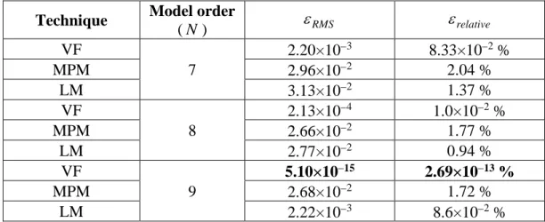
Table 4.1. Comparison of fitting accuracy for the analytical function (4.3) with N = . ... 603 Table 4.2. Comparison of fitting accuracy for the analytical function (4.3) using = 1 10−5 for
model order identification via MPM and LM techniques. ... 61 Table 4.3. Summary of the fitting errors for the analytical function (4.3) for different fitting
techniques and model orders. ... 62 Table 4.4. Comparison of fitting accuracy for the transformer case study with N = . ... 646 Table 4.5. Comparison of fitting techniques for the fitting of the admittance matrix of the circuit of
Figure 4.6. ... 67 Table 4.6. Parameters of the 225-kV cable system of Figure 4.15. ... 71 Table 4.7. Resulting model orders for different threshold values for the 225-kV cable system of
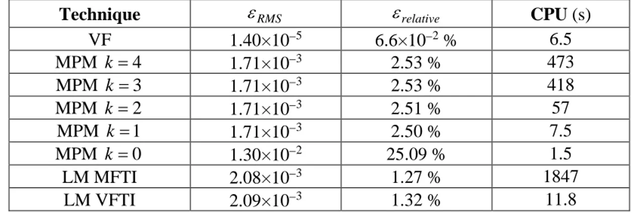
Figure 4.15. ... 71 Table 4.8. Fitting errors and CPU times for the fitting of the cable system of Figure 4.16 with fitting
order N =50, applying the VF, MPM and LM techniques. ... 73 Table 5.1. Comparison of the fitting accuracy by VF, MPM and LM for the fitting of the frequency-response of the distribution network of Figure 4.9 with different model orders. ... 78 Table 5.2. Model order identification by MPM and LM techniques applied to frequency-response
of the distribution network of Figure 4.9. ... 80 Table 5.3. Single-phase transmission line physical characteristics. ... 83 Table 5.4. Evaluation of the proposed techniques (MPM-VF and LM-VF) against MPM and LM
techniques applied to the distribution network case study of Figure 4.9. ... 85 Table 5.5. Fitting accuracy by the proposed approach (MPM-VF) for the fitting of the transmission
network system of Figure 5.8 with different values of . ... 88 Table 5.6. Evaluation of the RMS error by the proposed MPM-VF technique and the VF method
Table 6.1. Passivity enforcement by FRP, HMP and SDP methods for the FDNE of the distribution network case study with order N =60. ... 91 Table 6.2. Passivity enforcement performances by FRP, HMP and SDP methods for a rational
model with order N =100 for the 400-kV transmission network case study of Figure 5.8. . 91 Table 6.3. Complex-conjugate pair of poles with highest resonant frequencies for the rational
model with N =100 of the 400-kV transmission network. ... 93 Table 6.4. Comparison of the efficiency and fitting deviation by the PSRP, FRP, and HMP
techniques, for different model orders for the 400-kV transmission network FDNE. ... 101 Table 6.5. Comparison of the passivity enforcement techniques for different model orders for the
IEEE 39-Bus benchmark case study. ... 105 Table 6.6. Dominant poles for the passivity enforcement by the PSRP method for the 100-poles
FDNE for the IEEE 39-Bus benchmark case study. ... 107 Table 6.7. Comparison of the passivity enforcement techniques for different fitting bands for the
LIST OF FIGURES
Figure 1.1. Application of the FDNE approach. ... 1
Figure 1.2. 500-kV transmission network studied in [26], redrawn in EMTP. ... 5
Figure 1.3. 345-kV transmission network. ... 6
Figure 1.4. 225-kV Cross-bonded transmission cable system. ... 7
Figure 2.1. Time-invariant system. ... 12
Figure 2.2. Responses of a linear system. ... 13
Figure 3.1. Hamiltonian matrix perturbation scheme. ... 51
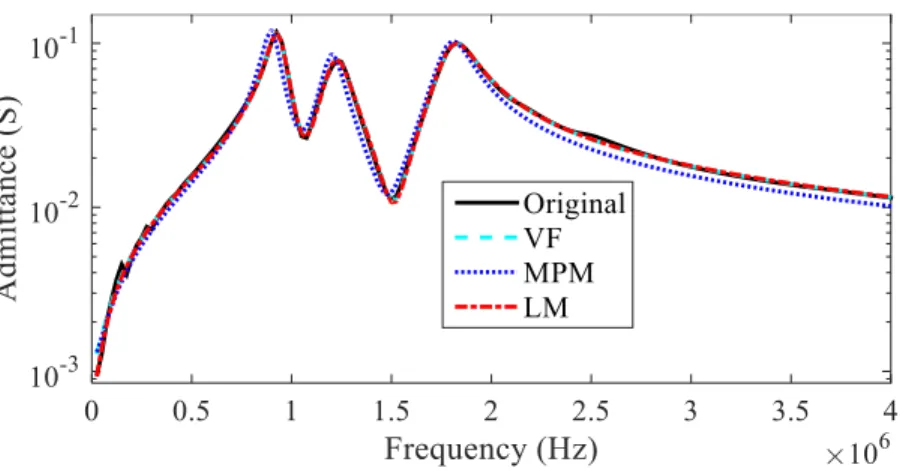
Figure 4.1. Magnitude of the frequency response of the analytical function (4.3) together with the fitted counterparts by VF, MPM and LM techniques. ... 59
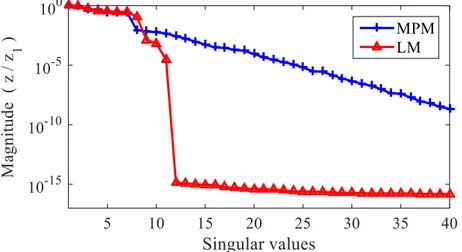
Figure 4.2. MPM- and LM-pencil singular values for the fitting of the function (4.3). ... 60
Figure 4.3. MPM-pencil singular values for the fitting of the function (4.3) with the asymptotic term d subtracted... 62
Figure 4.4. MPM- and LM-pencil singular values for the admittance function of the 11kV/230V transformer case study. ... 63
Figure 4.5. Magnitude fitting curves for the 11kV/230V transformer case study. ... 63
Figure 4.6. Pi circuit case study. ... 64
Figure 4.7. MPM- and LM-pencil singular values for the admittance matrix of the circuit of Figure 4.6. ... 65
Figure 4.8. Magnitude of the elements of the admittance matrix of the circuit of Figure 4.6 and fitted counterparts by the VF, MPM and LM techniques, (a) element Y
( )
1,1 , (b) element( )
1, 2 Y and (c) element Y( )
2, 2 . ... 66Figure 4.9. Distribution network case study, taken from [64]. ... 67
Figure 4.10. Magnitude of the elements of the admittance matrix of the distribution network of Figure 4.9 measured from nodes A and B. ... 68
Figure 4.11. MPM- and LM-pencil singular values for the admittance matrix of the distribution
network of Figure 4.9. ... 68
Figure 4.12. RMS error resulting from using different tolerance values via MPM and LM for the fitting of the distribution network of Figure 4.9. ... 69
Figure 4.13. Relative fitting errors by VF, MPM and LM, for different fitting orders for the fitting of the admittance matrix of the distribution network of Figure 4.9. ... 69
Figure 4.14. Cross-bonded cable subsection. ... 70
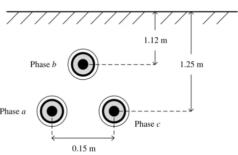
Figure 4.15. Geometry of the studied 225-kV cross-bonded cable system. ... 70
Figure 4.16. Magnitude of admittance matrix elements of the cross-bonded cable system. ... 71
Figure 4.17. MPM- and LM-pencil singular values for the admittance matrix of the cable system of Figure 4.15. ... 72
Figure 5.1. Convergence of the pole relocation process of the VF technique for the fitting of the transformer zero-sequence admittance. ... 77
Figure 5.2. Convergence of the pole relocation process of the VF technique for the fitting of the distribution network of Figure 4.9 with different model orders. ... 77
Figure 5.3. Eigenvalues of the conductance matrix of the VF-fitted model for the distribution network of Figure 4.9 with model orders: (a) N =40, (b) N =80 and (c) N =60. ... 79
Figure 5.4. Flowchart of the proposed combined fitting approach. ... 81
Figure 5.5. Magnitude plot by the proposed technique (LM-VF) for the transmission line case study, (a) characteristic admittance Yc
( )
s , (b) propagation function Γ( )
s . ... 84Figure 5.6. Comparison of the convergence of the pole relocation process by VF with different initial poles and the proposed approach (LM-VF), for the fitting of the characteristic admittance Yc
( )
s of the transmission line case study. ... 85Figure 5.7. Comparison of the convergence of the pole relocation process by the proposed approach (MPM-VF and LM-VF) against VF. ... 86
Figure 5.9. Magnitude of the admittance matrix entries Y
( )
1,1 and Y( )
1, 2 of the transmission network of Figure 5.8. ... 87 Figure 6.1. Eigenvalues of the conductance matrix of the original frequency-response and fittedrational model with N =100 for the 400-kV transmission network example. ... 92 Figure 6.2. Eigenvalues of the initially fitted (non-passive) and perturbed (passive) model for the
400-kV transmission network with N =100. ... 98 Figure 6.3. Illustration of multiple passivity violation intervals. ... 99 Figure 6.4. Iterative scheme proposed for the PSRP technique. ... 100 Figure 6.5. Admittance matrix elements of the external zone of the 400-kV transmission system of
Figure 5.8 together with their fitted counterparts. ... 102 Figure 6.6. Admittance matrix elements of the external zone of the 400-kV transmission system of
Figure 5.8 after passivity enforcement by the PSRP method. ... 102 Figure 6.7. Eigenvalues of the conductance matrix for the fitting of the 400-kV transmission system
of Figure 5.8 with N =150 before and after passivity enforcement by PSRP. ... 103 Figure 6.8. Time-domain simulation with passive 100-order FDNE model of 400-kV transmission
system; voltages at ADAPA bus. ... 103 Figure 6.9. Zoom of Figure 6.8. ... 104 Figure 6.10. IEEE 39-Bus benchmark. ... 105 Figure 6.11. Eigenvalues of the conductance matrix for the FDNE of the IEEE 39-Bus benchmark
with order N =90 before and after passivity enforcement by PSRP. ... 106 Figure 6.12. Eigenvalues of the conductance matrix for the FDNE of the IEEE 39-Bus benchmark
with order N =100 before and after passivity enforcement by PSRP. ... 106 Figure 6.13. Transient voltages at bus B3 of the network of Figure 6.10. ... 107 Figure 6.14. Zoom of the plot of Figure 6.13, phase b of the transient voltage at bus B3. ... 108 Figure 6.15. Eigenvalues of the conductance matrix of the cross-bonded cable system FDNE model
Figure 6.16. Zoom to the plot of Figure 6.15. ... 109 Figure 6.17. Transient voltage at phase a of bus m of the network of Figure 1.4. ... 110 Figure 6.18. Zoom of the transient voltage of Figure 6.17. ... 110
LIST OF SYMBOLS AND ABBREVIATIONS
BIBO Bounded-input bounded-outputCFIFT Closed-form inverse Fourier transform CPU Central processing unit
EMT Electromagnetic transients
EMTP Electromagnetic transient program
FD Frequency domain
FFT Fast Fourier transform FRP Fast residue perturbation
HMP Hamiltonian matrix perturbation HVDC High voltage direct current IFFT Inverse fast Fourier transform
LM Loewner matrix
LTI Linear time invariant MPM Matrix pencil method PRL Positive real lemma
PSRP Pole-selective residue perturbation ROC Region of convergence
SDP Semidefinite programming
TD Time domain
VF Vector fitting
LIST OF APPENDICES
Appendix A – State-space form of rational models ... 120 Appendix B – s-domain ROC for causal and BIBO-stable systems ... 123 Appendix C – Implementation of FDNEs in EMTP ... 125
CHAPTER 1
INTRODUCTION
The increasing complexity of modern electrical networks around the world has made essential the use of simulation software for electromagnetic transient (EMT) analysis. EMT-type simulations are widely used for design, operation and analysis of power systems. The large number of nodes in modern electrical networks, together with the complexity of its components results in very high computational burden for EMT-type simulations. This issue can be addressed using Frequency-Dependent Network Equivalents (FDNEs).
The computation of an FDNE requires to divide the network under study into study- and external-zone. The external zone is replaced by the FDNE as illustrated in Figure 1.1. The FDNE constitutes an equivalent reduced-order model of the external zone of the network, which allows the acceleration of time-domain computations. A restriction of FDNEs is that only linear and passive devices can be modelled.
In general, the calculation of FDNEs involves the following steps: 1. computation of the frequency response of the external zone of the network (impedance, admittance, scattering parameters or transfer function), 2. identification of the frequency response, normally achieved via a curve fitting technique, 3. passivity assessment of the identified frequency response and, if required, 4. passivity enforcement. The passivity condition is related to the inability of the model to generate energy, this condition is vital for the numerical stability of FDNE models in time-domain (TD) simulations. The FDNE approach is not a novel technique and many research works have been conducted on this topic. Thus, several techniques exist for the calculation of FDNEs and passivity enforcement as discussed in the literature review presented next.
Study zone
(Detailed models)
Port 1 Port 2 Port pExternal zone
(FDNE)
1.1 Literature review
Since the decade of 1950, some techniques to calculate the parameters of transfer functions of electrical systems from experimentally-obtained frequency responses have been developed; for example, [1-3] in the field of automatic control. In the field of power systems, those techniques were developed two decades later. In 1970, a Transient Network Analyzer (TNA) combined with digital computer for the simulation of open-end switching lines was developed [4]. The TNA consisted of a small-scale physical implementation used with a similar purpose than FDNEs. However, with the development of computers, the TNA looks impractical at present.
The calculation of FDNEs has emerged together with the necessity of accurately representing system components with distributed-parameters nature, such as transmission lines and transformers. In the decade of 1970, for example, a combination of resistive, inductive, and capacitive (RLC) elements in the form of interconnected cascade modules, were used for the representation of transmission lines [5, 6]. This technique was enhanced in 1980 and 1981 for lossless and lossy models, respectively [7, 8]. The same concept was utilized for the modeling of network equivalents for transient analysis in 1983, as reported in [9]. Using the same idea (RLC branches), but with a different procedure for the parameters determination, an alternative approach was proposed in 1984 in [10], and later extended to multiport systems in 1993 in [11].
A different approach for the computation of FDNEs, consisting of difference-equation models was proposed in [12] and [13, 14], published in 1993 and 2004, respectively. The difference-equation models are, however, limited to single-port systems, and for this reason they have never been very popular.
In 1993, an alternative technique to interface equivalent models by means of the Fast Fourier Transform (FFT) was proposed in [15]. This approach takes advantage of the delay produced by a transmission line to connect the study- with the external-zone. This technique is, however, very restrictive since a transmission line must be the breakpoint between the study- and external-zone. The Vector Fitting (VF) technique first appeared in 1998 for the modeling of transmission lines [16, 17]. In the same year, the application of the VF technique was extended to power transformers [18], and finally to FDNEs in 1999 [19]. A further analysis of the VF method, given in [20], recognizes the VF technique as an improved version of Sanathanan and Koerner method published
in 1963 [21]. Some improvements for the application of VF to multiport systems were published in 2002 for the fitting of admittance matrices in [22]. An alternative application of the VF technique in the z-domain was also proposed in 2007 in [23].
In 2003, a two-layer network equivalent was proposed [24]. In this approach, the external-zone is divided in two layers: a surface layer, consisting of a transmission line connected directly to the study-zone, and an inner layer, containing the rest of the network. The restriction of this technique is that it requires the surface layer to be a transmission line modeled as in [25].
Frequency-band partitioning was proposed in 2005 as an alternative fitting technique [26]. This frequency partitioning allows the computation of rational models via the solution of simple overdetermined system of equations. The reliability of this approach is however, dependent on the user’s expertise to define the frequency partitions.
In addition to the above-mentioned frequency-domain identification methods, dynamic equivalents can also be computed from time-domain responses. This is the case of the Matrix Pencil Method (MPM) [27], which was published in 1995, as an extension of [28]. Alternative time-domain identification approaches are the Prony method [29] and the TD-VF method [30], published in 1995 and 2003, respectively.
One of the most important questions in the computation of FDNEs is how to determine the fitting model order. Since 2010, a partial solution to this question was given by applying the MPM method in FD, as proposed in [31, 32]. Also, different Loewner-matrix based methods as reported in [33-35] include the model order identification feature. These techniques utilise singular value decomposition (SVD) to find a suitable model order. Moreover, these two techniques are non-iterative. Another model order identification method was proposed in 2016 [36]. This method consists of a combination of the Prony method with SVD.
As mentioned before, an essential requirement of FDNEs to perform numerically stable simulations is passivity. Passivity-guaranteed fitting methods are reported in [37] and [38], published in 2011 and 2017, respectively. In [37], genetic algorithms are applied to identify the coefficients of the equivalent model. On the other hand, the method in [38] consists of Brune’s realizations, which is an old approach, appeared around 1931 [39]. These passivity-guaranteed approaches are, however, only available for single-port systems.
Since the rest of existing fitting techniques cannot guarantee the passivity of FDNEs, a passivity assessment is always necessary, and if passivity violations are revealed, passivity must be enforced. Passivity can be assessed by computing the eigenvalues of the Hamiltonian matrix associated to the FDNE (state-space) model [40]. Alternatively, passivity can be assessed via the singularity test matrix [41]. As its name indicates, this matrix is half-size of the Hamiltonian matrix, then, it is computationally more efficient.
In the context of passivity enforcement, several methods have been reported in the literature. One of the most popular is the Fast-Residue Perturbation (FRP) technique, which consists of the solution of an optimisation problem via quadratic programming [42]. Another popular technique is the perturbation of the Hamiltonian matrix associated to the state-space representation of the rational model, which in turn, results in the perturbation of the state-space FDNE model [40]. Also, Positive Real Lemma (PRL) -based techniques have been proposed for passivity enforcement. Under this approach, the resulting optimization problem can be solved via Semidefinite Programming (SDP) as in [43]. A more recent approach was proposed in [44], which is an improved version of the SDP technique.
To conclude this literature review, it is remarked that there exist surveys about the computation of dynamic equivalents, some of them are given in [45-48], and chapter 10 of [49]. These references have been the primary source of information for this thesis.
1.2 Motivation
Although the use of FDNEs has been widely reported in the literature, and several approaches exist, the accuracy of the equivalent models relies on both, the techniques applied, and the user’s expertise. For example, a common user may utilize a very accurate fitting technique but a bad model order estimation, which can result in a poor accuracy of the approximation. Also, since FDNEs are prone to violate passivity, a suitable passivity enforcement technique should be selected and appropriately applied for accurate and stable solution. As it will be later demonstrated, in some cases, the existing passivity enforcement methods require large CPU times to enforce passivity, or in the worst scenario, they are unable to find a solution due to the large computational burden required. These issues constitute the main challenges and motivation of this thesis to create improved methods for the computation of FDNEs.
1.3 Scope
In this section, some important facts about the use of FDNEs are shown. Firstly, it is highlighted that with the development of computers and simulation software, some problems that used to be challenging in the past, are much easier to be solved nowadays. As preliminary example, the 500-kV transmission network used in [26] for the calculation of an FDNE, has been reproduced in EMTP [50]. The resulting draw is presented in Figure 1.2.
Figure 1.2. 500-kV transmission network studied in [26], redrawn in EMTP.
Capacitor bank External zone Study zone + 17.1kVRMSLL /_37.6?i AC1 + 7.96uH L1 + 0.0262 R1 + 18.1uH L2 1 2 +30 500/15 DY_1 1 2 +30 500/20 DY_2 + L5 0.160mH +C5 1nF 1nF +C6 + LD1 ?v 58,57.4mH + LD5 ?v 130,3.45mH + 16.5kVRMSLL /_12.4?i AC2 + 7.96uH L6 + 0.0262 R3 + 18.1uH L7 + LD2 ?v 86.6,86.6mH + 10mH L8 + 2.75 R4 + 0.587mH L9 + 6.27mH L3 + 0.367mH L4 + 1.72 R2 1 2 +30 500/15 DY_3 + 14.5mH L10 + 3.97 R5 + 0.847mH L11 + 16.5kVRMSLL /_10.4?i AC3 + 7.96uH L12 + 0.0262 R6 + 18.1uH L13 1 2 +30 500/15 DY_4 + 14.5mH ?i L14 + 3.97 R7 + 0.847mH L15 + LD6 ?v 129,3.41mH +C3 2650uF +C2 2650uF +C1 2650uF + LD4 ?v 14.8,6.71mH b a c b a c + 21.75kVRMSLL /_24.5?i AC4 + 7.96uH L16 + 0.0262 R8 + 18.1uH L17 1 2 +30 500/15 DY_5 + 4.89mH L18 + 1.34 R9 + 0.286mH L19 b a c b a c + LD3 ?v 85.1,89.4mH +C4 1nF + WB model WB_TL1 + W B m o d e l W B _ T L 5 + W B m o d e l W B _ T L 7 + W B m o d e l W B _ T L 6 + WB model WB_TL2 + WB model WB_TL3 + 1 2 3 4 5 6 WB model WB_TL4 +7.09ms|100|0 CB1 + 1|10|0?v CB2 BUS3 BUS6 a c BUS7 BUS8 BUS9 BUS2 BUS5 BUS4 BUS1 BUS10 BUS12 BUS11
Computing the TD simulation for the example of Figure 1.2 using a simulation time of 30 ms and a time-step of 5 μs, the resulting CPU simulation time is 0.32 s. Thus, it can be seen that the use of an FDNE is not worth it for this example since the simulation can be achieved very quickly. Another case where the application of FDNEs is not meaningful is the simulation of networks with highly-complex devices that cannot be included into the FDNE model, such as windfarms (WF) and HVDC systems. An example of such cases is the 345-kV network of Figure 1.3.
Figure 1.3. 345-kV transmission network.
SM PowerPlant_09 B38 SM PowerPlant_06 B35 SM PowerPlant_01 SM B31AndLoad SLACK PowerPlant_02 SM PowerPlant_03 B32 SM PowerPlant_05 B34 SM PowerPlant_04 B33 SM PowerPlant_07 B36 + 317.70 bus26_28 + 101.20 bus28_29 + 418.90 bus26_29 Load29 Load26 + 216.50 bus25_26 Load28 Load25 PI + b u s0 2 _ 2 5 5 8 km CP + b u s0 2 _ 0 3 1 0 1 .2 0 + b u s0 3 _ 1 8 8 9 .1 0 Load18 Load3 PI + b u s0 1 _ 0 2 2 7 6 km + b u s0 1 _ 3 9 1 6 7 .6 0 + b u s0 3 _ 0 4 1 4 2 .8 0 Load4 Load39 + b u s0 4 _ 0 5 8 5 .8 0 PI + b u s0 5 _ 0 6 1 7 km + b u s0 6 _ 0 7 6 1 .7 0 Load7 PI + 3 1 km b u s0 7 _ 0 8 + b u s0 5 _ 0 8 7 5 .1 0 + b u s0 9 _ 3 9 1 6 7 .6 0 + b u s0 8 _ 0 9 2 4 3 .3 0 Load8 + b u s2 6 _ 2 7 9 8 .5 0 + b u s1 7 _ 2 7 1 1 6 .0 0 PI + bus17_18 55km PI + b u s1 6 _ 1 7 60km PI + b u s1 6 _ 2 4 40km + b u s1 5 _ 1 6 6 3 .0 0 + b u s1 6 _ 2 1 9 0 .5 0 + b u s1 4 _ 1 5 1 4 5 .4 0 + b u s1 6 _ 1 9 1 3 0 .7 0 + b u s2 2 _ 2 3 6 4 .3 0 + b u s2 3 _ 2 4 2 3 4 .6 0 + bus21_22 93.80 + bus04_14 86.50 PI + b u s0 6 _ 1 1 5 5 km 2 3 1 xfo19_20 530/300/12.5 tap=1.06 1400MVA + b u s1 3 _ 1 4 6 7 .7 0 PI + 2 9 km b u s1 0 _ 1 3 PI + 2 9 km b u s1 0 _ 1 1 Load27 Load24 Load16 Load12 Load20 Load23 Load15 + BUS24_shunt 368uS 92MVAR@500kV Load21 F F a u lt BRKB3B4 BRKB4B3 1 2 -30 503/25 xf o 1 2 _ 1 3 200MVA tap=1.006 1 2 -30 503/25 xf o 1 2 _ 1 1 200MVA tap=1.006 offshore_WP 500kV / 220kV 500kV / 220kV onshore_WP B29 V1:1.04/_1.1 B28 V1:1.03/_-1.7 V1:1.02/_-3.8 B25 B7 V1:0.97/_-10.0 B39 V1:1.03/_-8.4 V1:1.02/_-9.3 B9 B8 V1:0.97/_-10.4 B27 V1:1.00/_-7.4 B26 V1:1.02/_-5.3 B17 V1:1.00/_-7.2 B18 V1:1.00/_-8.2 B23 V1:1.03/_0.6 B24 V1:1.01/_-6.0 B22 V1:1.04/_0.8 B21 V1:1.01/_-3.7 B6 V1:0.98/_-7.8 V1:0.99/_-6.1 B11 B19 V1:1.04/_-0.9 B13 V1:0.99/_-5.9 B10 V1:1.00/_-5.2 V1:0.98/_-2.0 300kV B20 V1:1.01/_-6.1 B16 B3 V1:0.99/_-8.5 B14 V1:0.99/_-7.5 B5 V1:0.98/_-8.5 V1:0.97/_-9.6 V1:0.99/_-7.7 B15 V1:0.96/_-36.1 B12 V1:0.97/_-9.6 B4 B1 V1:1.03/_-6.1 B2 V1:1.00/_-5.3
For the application of the FDNE approach in the test network of Figure 1.3, the study-zone must necessarily contain the WFs since those are nonlinear devices and they cannot be modeled by FDNEs. Different tests using FDNEs have been applied to this network; however, no substantial computational saving is achieved. The reason is that, most of the computational burden is demanded by the nonlinear devices, and since those are kept modeled in detail (inside the study-zone), the application of an FDNE cannot substantially accelerate the simulation.
An example that demonstrates the capabilities of FDNEs is the 225-kV cross-bonded cable system studied in [51] and shown in Figure 1.4. The cross-bonded cable of Figure 1.4 consists of 17 blocks, each of them containing 3 sections of the frequency dependent cable model based on [52]. The total cable length is 64 km and the shortest cable section propagation delay is 4.87×10⁻⁵ s. Further details about the cable modeling are given in [51, 53] and in section 4.6 of this thesis. For this example, it is important to remark that the simulation time-step cannot be larger than the above-mentioned (shortest) propagation delay.
Unlike other cable modelling techniques, such as the homogeneous model [52], the FDNE technique allows to tune the accuracy of the model by selecting the desired fitting frequency band and model order. Additionally, the use of an FDNE eliminates the restriction of the largest possible time-step, imposed by the shortest time-delay of the cable model.
Using a FDNE fitted for a frequency band from 1 Hz to 5 kHz, for a simulation time of 0.1 s and time-step of 4 μs, the CPU simulation time is reduced from 13 s to 0.59 s, i.e., an acceleration factor of 21 is obtained. Alternatively, using a time-step of 20 μs, the simulation CPU time can be reduced to 0.22 s, i.e. an acceleration factor of 58 is obtained.
Figure 1.4. 225-kV Cross-bonded transmission cable system.
Network equivalent SW Sheath grounding resistance Surge arrester Bus k Bus m +ZnO + + + + + + Cross-bonded cable +ZnO c b a c b a
Moreover, the use of FDNEs is especially advantageous for statistical studies. To cite an example, statistical studies are used for the determination of the maximum overvoltage due to a breaker switching, for which the simulations are repeated several times (50 times or more, for example) with different closing instants to find the critical voltage values.
The examples presented above show that the computational savings obtained by using FDNEs depend on several factors, such as number of nodes of the network, complexity of the models involved, number of connections ports, fitting frequency band, FDNE model order, simulation time, simulation time-step, among others. Therefore, it is emphasized that this thesis does not focus on the computational savings by using FDNEs since they depend on all the abovementioned factors. The scope of this thesis relies on the study of the FDNE modeling requirements, and the methodologies involved in the computation of FDNEs, such as fitting techniques, model order determination, and passivity enforcement.
Note that the simulation results presented in this chapter and all the simulation results presented in this thesis are achieved using a 16-GB of RAM, i7-4900MQ@2.80 GHz processor and 64-bit Windows operating system computer.
1.4 Contributions
The first contribution of this thesis consists of the proposal of a novel fitting procedure based on the Loewner-Matrix (LM) method. This new methodology is more straightforward than the traditional one in terms of extraction of unstable poles. Furthermore, the sparsity of the model obtained by the proposed strategy allows better computational efficiency in time-domain than the traditional LM technique. Subsequently, a comparative study of existing fitting techniques is presented. This study reveals some discoveries that had not been reported in the literature.
The second contribution of this thesis consists of a new fitting method that combines the Vector Fitting (VF) technique with either LM or the Matrix-Pencil-Method (MPM), which allows an easy model order identification and high fitting accuracy. The proposed technique achieves improved computational performance than the existing methods.
The third contribution of this thesis is the proposal of a novel passivity enforcement technique. Unlike existing methods, the proposed technique requires minimal computational effort, which make it advantageous for FDNEs with substantial number of connection ports and model order.
1.5 Thesis outline
Chapter 1 introduces the research topic, including a brief analysis about the computational savings by using FDNEs. This analysis defines the scope of the research.
In Chapter 2, the theoretical background for the calculation of FDNEs is presented, including: a study on the physical and mathematical requirements for FDNE modeling, such as linearity, causality and passivity.
Chapter 3 presents a review on: 1. Vector Fitting (VF), Matrix Pencil Method (MPM) and Loewner Matrix (LM) fitting techniques; 2. passivity assessment methods; and, 3. passivity enforcement techniques, such as the Fast Residue Perturbation (FRP), Hamiltonian Matrix Perturbation (HMP) and Semidefinite Programming (SDP) methods.
In Chapter 4, numerical analysis and comparisons between the VF, MPM and LM fitting techniques are presented. These studies reveal the capabilities and weakness of each technique. Also, some recommendations are given for the efficient application of the outlined methods. Different frequency-domain functions are fitted and analyzed in this chapter.
Based on the discoveries obtained in Chapter 4, a new fitting technique is proposed in Chapter 5. The proposed technique consists of a combination of the MPM or the LM method with the VF technique. The proposed technique is demonstrated to achieve better computational performance than the involved techniques applied individually.
In Chapter 6, the passivity enforcement techniques Fast Residue Perturbation (FRP), Hamiltonian Matrix Perturbations (HMP) and Semidefinite Programming, are first evaluated with some numerical examples, revealing their limitations. Then, a novel passivity enforcement technique, named Pole-Selective Residue Perturbation (PSRP) is presented. The proposed technique is demonstrated to achieve similar (slight) deviation of the rational model after passivity enforcement, while achieving a much better computational performance.
Finally, a summary of the work presented in this thesis is given in Chapter 7, followed by some ideas for future work.
CHAPTER 2
PRELIMINARIES ON RATIONAL MODELING
Rational modeling constitutes a powerful tool for reliable representation of dynamic systems in time-domain simulations. Dynamic systems can be usually represented by differential equations in time-domain. Sometimes, however, the determination of the differential equations for some devices/systems is not straightforward, such as the case of devices with distributed parameters nature. For those cases, rational modeling is an effective alternative.The process of calculating the coefficients of the rational model is known as identification process. This identification process is usually achieved by fitting the curve drawn by the frequency-response of the device/system under study. In the field of power systems, rational modeling is usually applied to frequency-dependent elements such as transmission lines/cables and transformers and to obtain frequency dependent network equivalents (FDNEs).
As revealed in the literature review given in Chapter 1, several fitting approaches have been proposed for the identification of dynamic systems; however, it is a tremendous task to study all the existing methods. This thesis focuses on the study of three of them: the VF, MPM and LM techniques. The VF is primarily considered since its use is very popular in both, research and industry applications. Moreover, the VF technique has been continuously improved. On the other hand, recent papers have been published about the MPM and LM methods, which demonstrate attractive features, such as, automatic model order determination, no need of initial poles guessing, and no need of iterative methods.
The VF, MPM and LM techniques produce rational/state-space models whose transfer function match the frequency response of the subnetwork or device being modeled over a finite frequency band. This frequency response can be given in admittance-, impedance-, scattering-parameters or transfer functions. Since this thesis focuses on FDNE modeling for EMT-simulations, admittance-parameters are of especial interest for compatibility with the EMTP software [50]. The rational models computed in this thesis are obtained using Matlab [54]. Note that the definitions given in this thesis for admittance-parameters also apply to impedance-parameters functions, whereas for transfer functions and scattering-parameters some definitions and/or modeling requirements, such as passivity may be slightly different.
Under the abovementioned considerations, the input data to the VF, MPM and LM techniques is the frequency-sampled admittance matrix
( )
( )
( )
( )
( )
11 1 1 p p pp y s y s s y s y s = Y , (2.1)where p denotes the number of ports, and the corresponding frequency points 1 Ns
s= s s , (2.2)
where s= j, =2 f being f the frequency in Hz and Ns is the number of frequency samples. The output model given by the VF and MPM fitting techniques is the rational model
( )
1 N n fitted n n s s s a = = + + −
R Y D E , (2.3)where coefficients an and Rn are denoted as the poles and residue matrices, respectively; D and E are constant matrices, which define the asymptotic frequency-response of the model; and N denotes the order of the model.
The rational model in (2.3) can equivalently be expressed in state-space form, which is also the model obtained by the LM method as
( )
t =( )
t +( )
tx Ax Bv , (2.4)
( )
t =( )
t +( )
t +( )
ti Cx Dv Ev , (2.5)
where the input vector v
( )
t denotes node voltages and the output vector i( )
t denotes branch currents. Thus, the fitted frequency-response can equivalently be expressed as the transfer function of the outlined state-space model as( )
(
)
1fitted s s s
−
= − + +
Y C I A B D E, (2.6)
where I denotes the identity matrix. The conversion from the rational model (2.3) to the state-space form (2.4)-(2.5) is given in Appendix A.
2.1 Modeling requirements
Both, the subnetwork or device to be modeled by a rational function as given in (2.3), or equivalently, by the state-space model as given in (2.4)-(2.5), and the equivalent model, must fulfill certain requirements for a realistic physical representation, such as time invariance, linearity, causality, stability, and passivity. These requirements are revisited next.
2.1.1 Time invariance
A system that produces an output signal y t
( )
due the input signal x t( )
is time invariant if the response due to a time-shifted input x t(
−)
is also time-shifted by the same period interval [55]. The time-invariance property is illustrated in Figure 2.1.Time-invariant system Time-invariant system
(
)
x t− y t(
−)
( )
x t y t( )
Figure 2.1. Time-invariant system.
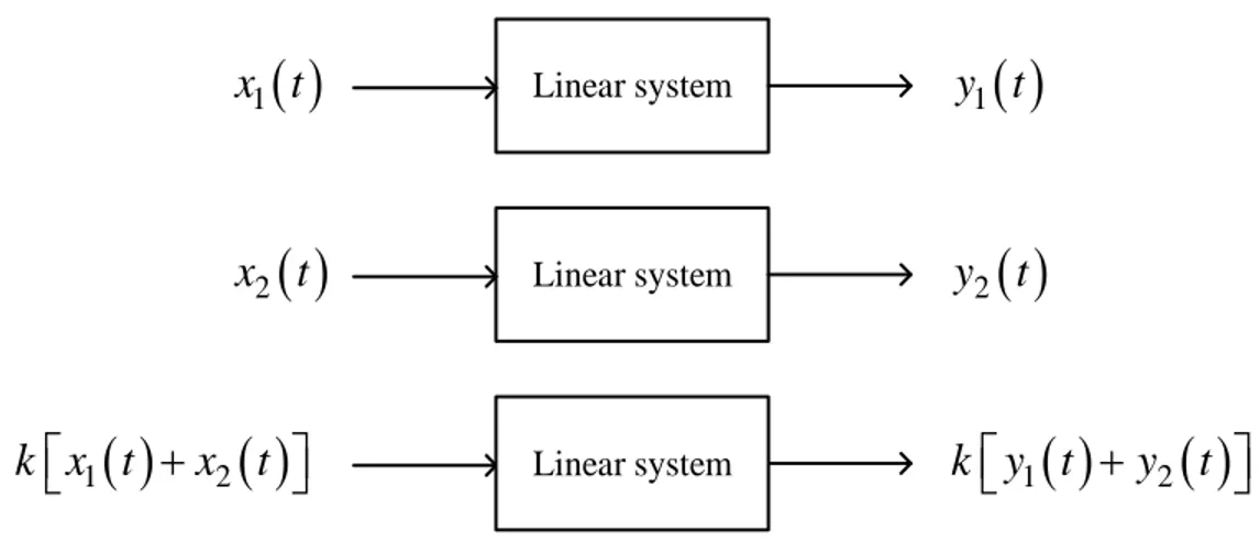
2.1.2 Linearity
A given system is linear if it satisfies the superposition principle [55]. To recall the superposition principle, let us consider that a given system produces the output signals y t1
( )
and y2( )
t due to the input signals x t1( )
and x2( )
t , respectively. Then, the system is linear if it produces an output( )
( )
1 2
y t +y t due to the input x t1
( )
+x2( )
t . Also, the system must satisfy the scalability condition, i.e., if the system receives an input signal kx t( )
, the output produced must be ky t( )
, being k an arbitrary scalar value. The linearity property is illustrated in Figure 2.2.The systems studied in this thesis are both linear and time invariant, which are usually referred in the literature as LTI systems.
Linear system
( )
( )
1 2k x t
+
x t
k y t
1( )
+
y
2( )
t
( )
1x t
y t
1( )
Linear system( )
2x
t
y
2( )
t
Linear systemFigure 2.2. Responses of a linear system.
2.1.3 Causality
Another important property of the systems studied in this thesis is causality. An LTI system is causal if it produces output signals that only depend on instantaneous and past (history) values of the applied input signal(s). In other words, a causal system cannot anticipate the response due to future input values [55].
The time-domain output of a single-port LTI system is given by the convolution integral
( )
( ) (
)
y t +h x t d −
=
− , (2.7)where x t
( )
and y t( )
denote the input and output signals, respectively, and h t( )
denotes the impulse response of the system. For a causal system, h t( )
must respect the following condition( )
0h t = , . t 0 (2.8) Supossing that an input is applied to the system at time t = , the causality condition in (2.8) 0 ensures that the system will have null response for negative times in (2.7). For multiport systems, this condition applies to every element of the corresponding impulse response matrix, also referred in the literature as transfer matrix.
The bilateral Laplace transform of h t
( )
, denoted in this thesis as H s( )
is the transfer function( )
( )
, stH s +h t e− dt −
It is recalled that the Laplace transform of any TD signal exists, if and only if, the integral given at the right side in (2.9) converges to a finite value. Thus, the Laplace transform of any signal may be defined for certain values of s and not for others. The set of values of s for which the Laplace transform integral converges is known as the region of convergence (ROC).
For time-domain signals whose response is zero for t , such as 0 h t
( )
of a causal system, the ROC only comprises the right half side of the complex plane (
s 0: s ), the demonstration is given in Appendix B of this thesis. This condition implies that the transfer function H s( )
of a causal system must be defined for
s 0: s . Non-causal systems are unrealizable in real-life systems, and they are not considered in this thesis. Furthermore, the rational model studied in this thesis, as defined in (2.3), is always defined for
s 0: s . Moreover, when this model is discretized and implemented in domain simulations, the output of the model at every time-step is only dependent on past (history) and present values of the input(s). Thus, the system described by the rational model (2.3) is considered causal.2.1.4 Stability
2.1.4.1 Input-output stability
An LTI system is said to be stable if for any magnitude-bounded input, defined as
( )
x t K , , t (2.10)
a magnitude-bounded output is obtained at any time, i.e.,
( )
y t M , , t (2.11)
where K and M are real scalar values. This condition is also known as BIBO (bounded-input bounded-output) stability [55].
The requirement for an LTI system to be BIBO stable is that its impulse response h t
( )
must be bounded and finite as t → . This is equivalent to state that the impulse response of a BIBO system is integrable, i.e.,( )
h t dt +
−
. (2.12)This condition guarantees that for any bounded input x t
( )
with finite duration (applied up to a certain time t ), the output will be bounded and it will have a transient nature, i.e., it will vanish as t → .The condition for BIBO stability given in (2.12), can be also analyzed in the frequency-domain by analyzing the Laplace-Transform ROC of h t
( )
. As demonstrated in Appendix B, the ROC of h t( )
of a causal system only includes the right-half complex plane without including the imaginary axis; however, if causality and BIBO stability features are combined, the ROC also includes the imaginary axis. The proof is also provided in Appendix B.Then, a necessary condition for causal and BIBO stable systems is that the transfer function H s
( )
or H( )
s for multiport systems, must be defined, analytic and bounded for
s 0: s . Note that in this section we use H( )
s as a generic transfer function, although the transfer function studied in this thesis is an admittance-parameters matrix, denoted as Y( )
s .2.1.4.2 Internal stability
Another (equivalent) stability analysis can be achieved in terms of the internal constitution of the state-space model as given in (2.4)-(2.5) or, equivalently, the rational model given in (2.3). The requirement for this model to be stable is that all the poles must have negative real part.
To demonstrate the importance of this fact, let us use a generic residue-pole element of the rational model (2.3) for an arbitrary entry of the generic transfer function H
( )
s , i.e.( )
r H ss a
=
− (2.13)
and its time-domain representation (according to the inverse Laplace transform) as
( )
ath t =re . (2.14)
( )
j 0tu t =e , (2.15)
where is the angular frequency, the resulting output becomes 0
( )
( ) ( )
at j 0ty t =h t u t =re e . (2.16)
where denotes convolution.
From (2.16), it can be inferred that the requirement for the output y t
( )
to be bounded is that the convoluted signals h t( )
and u t( )
must be both, bounded. Since the input signal has been set as a sinusoidal function, it is bounded. On the other hand, the condition for h t( )
to be bounded, considering the general case in which a is a complex value, is that the real part of a must be negative, otherwise, h t( )
would be an exponentially growing function (unbounded).This condition can be alternatively analyzed from (2.14) as follows. If the real part of a is negative, the impulse response (2.14) vanishes for t → , such that h t
( )
is integrable, satisfying the condition in (2.12) for BIBO stability.2.1.5 Passivity
The most challenging requirement to fulfill when computing rational models, such as for FDNEs, is passivity. A passive system is defined as a system that can absorb energy at any time, but it can only deliver energy if some energy was previously stored in it, and this delivered energy cannot exceed the amount of energy previously stored in it at any time [56]. This definition can be analyzed in terms of power and energy as follows.
The instantaneous power absorbed by the dynamic system given in (2.4)-(2.5) is:
( )
( ) ( )
Tp t = v t i t . (2.17)
Based on (2.17), the cumulative energy absorbed by the system up to the arbitrary time ta is
( )
ta( )
,E t p t dt −
=
. (2.18)( )
0E t , . t (2.19) This definition is, however, useless in practice since it requires analyzing specific pairs of input and output signals, and it is impossible to analyze all the possible inputs to a given system. Also, it is important to consider that for a non-passive model, the time-domain simulation can be numerically unstable, such that output variables can be meaningless.
Alternatively, the instantaneous power entering a generic multiport system as given in (2.17) can be expressed in terms of frequency-domain variables, i.e.
( )
( ) ( )
H
( )
H( ) ( )
p t = V s I s = V s Y s V s . (2.20)
where V
( )
s and I( )
s are the vectors of voltages and currents, respectively, and Y( )
s is the admittance matrix represented by a rational model. This expression can be rewritten as( )
( )
T s t( ) ( )
st
p t = V s e Y s V s e , (2.21)
or, in a simpler form
( )
T( )
2 s t p t = u Y s u e , (2.22) where( )
s = u V . (2.23)Considering (2.22), the cumulative energy up to an arbitrary time t as defined in (2.18) is a
( )
( )
,
( )
2
2 a s t t T e E t p t dt s s − = =
u Y u , (2.24)where the condition
s 0 must be respected to guarantee the integral’s convergence. According to (2.19), the system represented by Y( )
s is passive if and only if its cumulative energy is nonnegative at any time. From (2.24), it can be observed that neither the term
2 2 s t e s , nor ucan make E t
( )
0. Thus, the passivity condition relies on the nonnegative definiteness of the admittance matrix Y( )
s [56]. This condition can be mathematically defined as( )
( )
1 0 2 H s s + Y Y ,
s 0. (2.25)The left side of the inequality in (2.25) denotes the Hermitian part of Y
( )
s . In the case of Y( )
s being symmetric, the Hermitian part of Y( )
s is equal to its real part, or equivalently the conductance matrix G( )
s . From (2.25), it can be stated that a multiport system represented by the admittance matrix Y( )
s is passive if and only if its Hermitian part is nonnegative definite for the right-half side of the complex plane.The nonnegative definiteness of Y
( )
s as indicated in (2.25) is equivalent to requiring the Hermitian part of Y( )
s to have all its eigenvalues nonnegative, i.e.,( )
( )
eig Y s +Y s H 0,
s 0. (2.26)2.1.6 Positive real matrix theorem
So far, the conditions for causality, stability, and passivity of rational models based on the Laplace transform have been revisited. These conditions can be equivalently verified using the Fourier transform [56, 57], which is a particular case of the Laplace transform where the real part of the complex variable s= + j is zero, i.e., s= j. Using the Fourier transform the conditions for causality, stability and passivity stand as for the Laplace domain, but they must be fulfilled only for the imaginary axis, i.e., s= j, instead of all the right-half complex plane.
Considering the Fourier transform, the positive real theorem for rational matrices englobes the previously studied conditions for causality, stability and passivity as follows.
A rational matrix represented by Y
( )
s , where s= j, is positive real if and only if 1. Y( )
s is defined and analytic for 03. Y
( )
s =Y( )
−s4. Y
( )
s +Y( )
s H 0, 5. Y
( )
s →sE when s → , E being constant, real, symmetric and nonnegative definite. A quick analysis of the positive real matrix theorem reveals that the first and second points imply stability and causality of the rational model denoted by Y( )
s ; the third point guarantees that the impulse response is only real; the fourth point is the requirement for the rational model to be passive; finally, the fifth point establishes the asymptotic behaviour of the system.Then, the positive real theorem summarizes the requirements of rational models for stable, causal and passive characterization of LTI systems, as required for FDNE modeling. Each point of this theorem is, however, not necessarily tested when computing a rational model. The fitting techniques studied in this thesis guarantee the symmetry of the model; also, the generated poles are forced to have negative real part. On the other hand, the nonnegative definiteness of the model (fourth point), which is the condition for passivity, cannot be guaranteed.
It is important to mention that the positive real theorem stands for rational model without purely imaginary poles, such case requires a special treatment [56]. The methodologies presented in this thesis do not produce rational models with purely imaginary poles.
2.1.7 Positive real lemma
The positive real lemma gives an alternative method for evaluating the passivity of a state-space model from a point of view of dissipative energy. Let us consider a generic function V
(
x( )
t)
as the function of the energy storage by a system at any time. According to (2.18), the change of energy (or cumulative energy) in the system for a period of time
t0 t1
can be expressed as( )
( )
1( )
( )
( )
0 1 0 , 1 0 t t Vx t −V x t
p t dt=E t −E t , ,t0 t1 (2.27) where x( )
t denotes the state vector of the state-space model under study. Equation (2.27) implies that the energy stored during a given period of time can never exceed the cumulative energy E t( )
during that period. This definition is consistent with the passivity definition given in section 2.1.5.Then, dividing (2.27) by the time interval
(
t1−t0)
→0 the following expression is obtained dV( )
t p t( )
dt x . (2.28)According to the Lyapunov stability criterion [56], it is sufficient to consider the quadratic storage function
( )
( )
T( )
Vx t =x t Px t :P=PT 0 (2.29) to evaluate the system passivity. Then, the derivative of (2.29), as required in the left side of (2.28) becomes
( )
1(
( ) ( ) ( )
( )
)
2 T T dV t t t t t dt x = + x Px x Px , (2.30)and the power absorbed by the system, as given at the right side of (2.28) can be expressed as
( )
1( ) ( ) ( ) ( )
2
T T
p t = v t i t +i t v t . (2.31)
Substituting (2.30) and (2.31) in (2.28) results into
( ) ( ) ( )
T( )
( ) ( ) ( ) ( )
T T Tt t + t t t t + t t
x Px x Px v i i v , (2.32)
Substituting the state-space model equations (2.4) and (2.5) in (2.32), the inequality becomes
+
T + T
+
T
+
+ +
TAx Bv Px x P Ax Bv v Cx Dv Cx Dv v. (2.33)
After some algebraic manipulations, (2.33) can be written as
(
)
0 T T T T T T + − − − + A P PA PB C x x v v B P C D D . (2.34)Finally, considering (2.34) and the constraint condition P=PT 0 in (2.29), the positive real lemma is derived as follows:
The system described by the state space model (2.4)-(2.5) is passive, if and only if 0 T =P P such that
(
)
0 T T T T + − − − + A P PA PB C B P C D D . (2.35)Both, the positive real matrix theorem and the positive real lemma, give sufficiency conditions to claim passivity of rational models.
2.2 Conclusions
This chapter presents an overview on the physical and mathematic requirements for rational modeling, such as linearity, causality, stability and passivity. As it is studied in this chapter, the most challenging requirement to fulfill is passivity, which can be guaranteed if the rational model respects the positive real matrix theorem or the positive real lemma, which give sufficient conditions for passivity.
CHAPTER 3
RATIONAL MODELING TECHNIQUES
3.1 Fitting techniques
In this section, the theories of Vector Fitting (VF), Matrix Pencil Method (MPM), and Loewner matrix (LM) techniques are reviewed. This review sets the basis for further studies about fitting presented in Chapter 4.
3.1.1 Vector Fitting Technique
To start with the analysis of the VF method, the fitting of a generic scalar function f s
( )
is first analyzed. This case is equivalent to the fitting of the frequency-response of a single-port system. The corresponding fitted model (scalar case of (2.3)) is( )
1 N n fitted n n r f s d se s a = = + + −
. (3.1)The VF technique computes the rational model (3.1) in two stages. In the first stage, the poles of the system (an) are computed, in the second stage, the residues rn, and asymptotic terms d and e are obtained.
3.1.1.1 Poles computation
In the first stage of the original VF technique [19], the poles of the system are obtained in an iterative relocation process from an initial (guessed) set of poles, denoted in this thesis as an. As for this first version of the VF technique, VF introduces the auxiliary function
( )
1 1 N n n n c s s a = = + −
, (3.2)to create the augmented problem