Mathematical modeling in elastography.

HAL Id: pastel-00004165

https://pastel.archives-ouvertes.fr/pastel-00004165

HAL is a multi-disciplinary open access archive for the deposit and dissemination of sci-entific research documents, whether they are pub-lished or not. The documents may come from teaching and research institutions in France or abroad, or from public or private research centers.

L’archive ouverte pluridisciplinaire HAL, est destinée au dépôt et à la diffusion de documents scientifiques de niveau recherche, publiés ou non, émanant des établissements d’enseignement et de recherche français ou étrangers, des laboratoires publics ou privés.

To cite this version:

Anastasia Kozhemyak. Mathematical modeling in elastography.. Mathematics [math]. Ecole Poly-technique X, 2008. English. �pastel-00004165�

Th`ese pour l’obtention du titre de

DOCTEUR DE L’´ECOLE POLYTECHNIQUE Sp´ecialit´e : Math´ematiques Appliqu´ees

pr´esent´ee et soutenue par Anastasia KOZHEMYAK

Mathematical Models and Reconstruction Methods

for Emerging Biomedical Imaging Techniques

Jury

Ioan IONESCU (Pr´esident du jury) Mark ASCH (Rapporteur)

Vilmos KOMORNIK (Rapporteur) Habib AMMARI (Directeur de th`ese) Kamel HAMDACHE (Examinateur)

Roman NOVIKOV (Examinateur)

´

ECOLE POLYTECHNIQUE – CENTRE DE MATH´EMATHIQUES APPLIQU´EES

Remerciements

Je tiens en premier lieu `a remercier tr`es chaleureusement Habib Ammari, mon directeur de th`ese, pour son soutien au cours de ces quatre ann´ees. Son ouverture scientifique, sa rigueur, son enthousiasme toujours tr`es communicatif, ses critiques et ses encouragements sont pour beaucoup dans ce travail.

Je remercie tous les membres du jury du temps qu’ils m’ont consacr´e. Mes remerciements vont tout particuli`erement `a Marc Asch et `a Vilmos Komornik qui ont accept´e la tˆache de rapporteur. Ma reconnaissance va ´egalement `a Ioan Ionescu pour avoir accept´e la pr´esidence de mon jury.

Je voudrais exprimer ma reconnaissance `a Sylvain Ferrand pour son aide en informatique. Toute ma gratitude va `a toutes les autres personnes qui m’ont aid´ee et qui ont contribu´e `a l’enrichissement de ce travail.

Je termine ici en d´ediant ce m´emoire `a toute ma famille pour leurs encouragements pr´ecieux et en particulier `a Alexey et `a Ivan pour leur patience.

Contents

1.2.1 Vibration Potential Tomography . . . 18

1.2.2 Magneto-Acoustic Tomography with Magnetic Induction . . . 21

1.2.3 Magneto-Acoustic Current Imaging . . . 22

1.3 Reconstruction Methods . . . 22

1.3.1 Reconstruction Methods for the VPT . . . 22

1.3.2 Reconstruction Method for the MAT-MI . . . 25

1.3.3 Localization Method for the MACI . . . 28

1.4 Examples of Applications . . . 28

1.4.1 Vibration Potential Tomography with FreeFem++ . . . 28

1.4.2 Magneto-Acoustic Tomographies with Incomplete Data . . . 30

1.5 Concluding Remarks . . . 30

2 Thermography Based Recovery of Anomalies 33 2.1 Introduction . . . 33

2.2 Physical Background and Green’s Function . . . 35

2.2.1 Problem Statement . . . 35

2.2.2 Non-dimensionalisation . . . 35

2.2.3 Properties of the Solution to the Perturbed Problem . . . 36

2.2.4 Green’s Function and Solution to the Unperturbed Problem . . . 37

2.3 The Perturbed Temperature Field . . . 39

2.3.1 A Preliminary Result . . . 39

2.3.2 Equations for the Perturbed Part of the Temperature Field . . . 40

2.3.3 The Correction Term . . . 40

2.4 The Two-Dimensional Case . . . 43

2.4.1 Straightforward Modifications of Green’s Function to Fit the 2D Case 43 2.4.2 Special Corrector Obtained by Introducing a Cut off Function . . . 44

2.4.3 Derivation of the Order of the Estimate . . . 45

2.5 Asymptotic Expansion . . . 47

2.6 Examples of Applications . . . 48

2.6.1 Active Temperature Imaging . . . 48

2.8 Concluding Remarks . . . 55

3 Electrical Impedance Endo-Tomography 57 3.1 Introduction . . . 57

3.2 Mathematical Model . . . 59

3.3 Detection of Anisotropy . . . 61

3.3.1 Green’s Function, Single and Double Layer Potentials . . . 61

3.3.2 Anisotropic Polarization Tensors . . . 61

3.3.3 Detection of First-Order APT . . . 63

3.3.4 APT for Ellipses . . . 64

3.3.5 Anisotropy Detection . . . 65

3.3.6 Numerical Tests . . . 67

3.4 EIET by Elastic Deformation . . . 68

3.4.1 Physical Model . . . 68

3.4.2 Mathematical Model . . . 69

3.4.3 Conductivity Recovery . . . 70

3.5 Electrode Model . . . 72

3.5.1 Physical Principles . . . 72

3.5.2 Detection of the Centers and the Radius of the Anomalies . . . 75

3.5.3 Numerical Tests . . . 76

3.6 Concluding Remarks . . . 79

Bibliography 81

Introduction

Pr´

esentation g´

en´

erale

L’apparition de techniques avanc´ees en imagerie a am´elior´e de mani`ere significative la qualit´e de la surveillance m´edicale des patients. Les modalit´es d’imagerie non-invasives permettent aux m´edecins de faire des diagnostics plus pr´ecis et plus pr´ecoces et de prescrire des modes de traitement plus performants et plus justes. De multiples modalit´es d’imagerie sont employ´ees actuellement ou sont en cours d’´etude.

Dans cette th`ese, nous ´etudions trois techniques ´emergentes d’imagerie biom´edicale : • imagerie magn´eto-acoustique;

• imagerie thermographique;

• endotomographie par imp´edance ´electrique.

Pour chacune de ces trois techniques, nous proposons des mod`eles math´ematiques et nous pr´esentons des nouvelles m´ethodes de reconstruction en imagerie m´edicale.

Tout d’abord, nous allons d´ecrire les principes physiques de toutes les techniques propos´ees dans cette th`ese.

En imagerie magn´eto-acoustique, le signal de sonde, par exemple une onde acoustique, un courant ´electrique ou une tension ´electrique, est appliqu´e aux tissus biologiques qui sont plac´es dans un champs magn´etique. Le signal induit par la force de Lorentz est une fonction de la conductivit´e locale des tissus biologiques. Si, par exemple, le signal de sonde est une onde acoustique alors le signal induit est un courant ´electrique et la force de Lorentz produit l’apparition d’une densit´e de courant ´electrique locale.

La mesure des courants ´electriques (a) ou de la pression (b) induits sur l’ensemble de la fronti`ere, proportionnels `a la conductivit´e locale, permet d’obtenir la distribution de la conductivit´e avec une bonne r´esolution. La m´ethode (a) est appel´ee l’imagerie

potentielle par vibration ou VPT (de l’anglais vibration potential imaging) aussi connue

comme l’imagerie `a effet Hall. La m´ethode (b) est appel´ee la tomographie

magn´eto-acoustique `a induction magn´etique ou MAT-MI (de l’anglais magneto-acoustic tomography with magnetic induction).

La m´ethode (a) peut ˆetre appliqu´ee aux tissus du corps in vivo, ainsi qu’aux cellules cultiv´ees en suspension. Le faisceau ultrasonore effectue l’excitation dans une r´egion d’´etude et le courant induit est mesur´e `a l’aide des ´electrodes. La recherche dans cette direction semble tr`es prometteuse pour avancer la tomographie par imp´edence ´electrique ou EIT (de l’anglais electrical impedance tomography). La technique EIT est une technique d’imagerie qui se concentre sur la reconstruction de la distribution de l’imp´edance dans les tissus biologiques par l’injection de courants ´electriques et par la mesure non-invasive de potentiels. Dans le cadre de la technique EIT, le courant ´electrique est inject´e dans l’objet par les ´electrodes surfaciques et les potentiels correspondant `a la fronti`ere sont mesur´es sur toute la surface de l’objet dans le but de reconsrtuire la distribution de l’imp´edance `a l’int´erieur de l’objet. Il est bien connu que cette m´ethode d’imagerie de la distribution de conductivit´e produit des r´esultats avec une mauvaise pr´ecision. L’imagerie potentielle par vibration s’appuie sur des techniques de mesure innovantes qui int`egrent l’information structurelle. Dans le cadre de cette m´ethode, la r´esolution intrins`eque est de l’ordre de la taille de la tˆache focale de l’onde ultrasonore, alors elle devrait fournir des r´esultats de haute r´esolution.

Notons qu’une onde acoustique ou un d´eplacement de tissu apparaissent lorsque l’on place un tissu ´electriquement actif dans un champs magn´etique.

Cette m´ethode (c), appel´ee l’imagerie magn´eto-acoustique de courant ´electrique ou MACI (de l’anglais magneto-acoustic current imaging), a ´et´e propos´ee pour reconstruire les conductivit´es en detectant les courants actifs r´esultants de l’action de nerfs ou de fibres musculaires qui peuvent ˆetre imag´es en mesurant le signal de pression induit.

L’imagerie m´edicale thermique est en train de devenir une modalit´e de d´epistage du cancer du sein, de la peau et du foie. En tant que modalit´e d’imagerie physiologique qui effectue les analyses sur les fonctions du corps, elle peut permettre un diagnostic plus pr´ecoce que des examens anatomiques. La proc´edure de l’imagerie m´edicale thermique est fond´ee sur le principe selon lequel l’activit´e des vaisseaux sanguins et lymphatiques dans le tissu pr´ecanc´ereux et dans la zones environnantes du cancer d´evelopp´e est presque toujours plus ´elev´ee que dans les tissus normaux. Comme les masses pr´ecanc´ereuses et canc´ereuses sont des tissus tr`es m´etaboliques, ils ont besoin de ravitaillement abondant pour maintenir leur croissance. Pour croˆıtre les tumeurs doivent d´evelopper un nouveau circuit d’approvisionnement sanguin. En effet, les tumeurs induisent un tel syst`eme de nouveaux vaisseaux sanguins `a partir de vaisseaux pr´eexistants, processus qui se rap-porte `a l’angiogen`ese. Ce processus se traduit par une augmentation de la temp´erature. L’exp´erience actuelle consiste `a utiliser des cam´eras thermiques ultra-sensibles et des ordinateurs sophistiqu´es pour d´etecter, analyser et produire des images thermiques de diagnostic haute r´esolution des changements de temp´erature et vasculaires.

Le principe de l’imagerie thermique est le suivant. Un d´etecteur infrarouge `a balayage est utilis´e pour convertir le rayonnement infrarouge ´emis par la surface de la peau en impulsions ´electriques qui sont visualis´ees en couleurs sur un moniteur. Cette image visuelle, appel´ee thermogramme, repr´esente graphiquement la temp´erature du corps. Comme dans le corps normal la r´epartition de la temp´erature est assez sym´etrique, la r´epartition anormale de temp´erature peut ˆetre facilement identifi´ee.

Les ´etudes cliniques montrent que l’imagerie thermique des seins a une sensitivit´e et pr´ecision de 90% en moyenne. Une image infrarouge anormale est le plus important marqueur de risque ´elev´e de d´eveloppement du cancer du sein. L’imagerie thermique peut ˆetre utilis´ee

(i) pour d´efinir l’´etendue de la l´esion dont le diagnostic a ´et´e d´ej`a fait;

(ii) pour la localisation d’un domaine anormal non pr´ealablement identifi´e, dans le but d’effectuer les tests de diagnostique suivants;

(iii) pour d´etecter pr´ecocement les l´esions avant qu’elles ne soient cliniquement ´evidentes;

(iv) pour guider les th´erapies parmi lesquelles les plus connues sont les nouvelles tech-niques de thermo-ablation des tumeurs.

L’imagerie thermique ultrasonore est une technique prometteuse qui utilise la thermogra-phie. Elle exploite le principe de d´ependance de la vitesse du son dans un milieu vis-`a-vis de la temp´erature. Les techniques de thermo-ablation, telle que la chirurgie par ultrasons focalis´es, vise `a d´etruire les tumeurs malignes sans endommager les tissus environnants. La technique consiste, dans un premier temps, `a utiliser le syst`eme de la chirurgie par ultrasons focalis´es `a basse intensit´e et utiliser en mˆeme temps le syst`eme de diagnostique d’imagerie thermique ultrasonore pour d´etecter l’augmentation locale de la temp´erature en supposant que la d´ependance de la vitesse du son vis-`a-vis de la temp´erature est connue. L’endotomographie par imp´edance ´electrique ou EIET (de l’anglais electrical

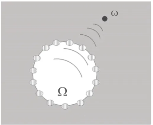
impe-dance endo-tomography) est une m´ethode pour reconstruire la conductivit´e des tissus ou

des organes profonds en utilisant une sonde d’imp´edance situ´ee au centre de la r´egion d’´etude. La sonde est constitu´ee d’´electrodes parall`eles, plac´ees `a la surface d’un cylindre isolant et le champ ´electrique se propage dans le milieu entourant la sonde. Cette nouvelle m´ethode a ´et´e d´eveloppee pour la d´etection du cancer de la prostate. Le principe de l’endotomographie suppose que le tissu normal de la prostate et le tissu de la tumeur ont des conductivit´es ´electriques tr`es diff´erentes.

Dans la pratique, le nombre des couples de courants et des potentiels ´electriques captur´es doivent ˆetre limit´es en fonction du nombre d’´electrodes fix´ees sur la surface de la sonde ce qui restreint la r´esolution de l’image. Nous pouvons certainement augmenter la r´esolution de l’image de conductivit´e en augmentant le nombre d’´electrodes. N´eanmoins, il faut remarquer qu’au-del`a d’un certain niveau, l’augmentation du nombre d’´electrodes ne peut pas am´eliorer la r´esolution de l’image `a l’int´erieur du corps `a cause de l’in´evitable bruit de mesure et de l’insensibilit´e intrins`eque mentionn´ee auparavant. Dans sa forme la plus

g´en´erale EIET est s´ev`erement mal pos´ee et non lin´eaire. Ces difficult´es majeures et fondamentales peuvent ˆetre mises en ´evidence par les propri´et´es de la valeur moyenne dans le cadre de la th´eorie des ´equations aux d´eriv´ees partielles elliptiques. En effet, la valeur du potentiel `a chaque point dans le milieu environnant la sonde peut ˆetre exprim´ee comme une moyenne pond´er´ee de potentiels voisins o`u le poids est d´etermin´e par la distribution de conductivit´e. Dans ce mode de calul de moyenne pond´er´ee, les valeurs de potentiels mesur´ees par la sonde sont influenc´ees par la distribution de conductivit´e. Par cons´equent, les mesures de la sonde sont reli´ees `a la distribution de conductivit´e de fa¸con fortement non lin´eaire. C’est le principal obstacle au d´eveloppement des algorithmes de reconstruction non-it´eratifs en pr´esence de limitation de donn´ees. Cependant, si nous avons d’autres informations structurelles sur le milieu, alors nous pourrons peut-ˆetre d´eterminer les caract´eristiques sp´ecifiques sur la distribution de conductivit´e avec une bonne r´esolution. Par exemple, on peut supposer qu’il existe un certain nombre de petites inclusions de conductivit´es nettement diff´erentes de celle du fond. Cette situation se pr´esente par exemple dans le cadre de l’imagerie du cancer de la prostate.

Dans ce cas, EIET cherche `a restituer les inclusions inconnues. Grˆace `a la petite taille des inclusions les potentiels associ´es mesur´es `a la surface de la sonde sont tr`es proches de potentiels correspondant au milieu sans inclusions. A moins que l’on sˆache exactement quel ´echantillon doit ˆetre restitu´e, il est presque impossible d’extraire de donn´ees largement bruit´ees des informations pertinentes sur les inclusions. En outre, en imagerie de la prostate, il n’est en g´en´eral pas n´ecessaire de reconstituer la conductivit´e ou de reconstruire la g´eom´etrie des inclusions avec une tr`es grande pr´ecision. L’int´erˆet majeur consiste `a d´eterminer leurs positions et leurs tailles.

Plan de la th`

ese

Dans le chapitre 1, apr`es avoir rappel´e les bases th´eoriques des trois approches diff´erentes de l’imagerie magn´eto-acoustique, nous proposons de nouveaux algorithmes pour r´esoudre des probl`emes inverses correspondant `a chaque approche.

Le chapitre 2 est consacr´e `a l’imagerie thermographique. Nous effectuons une ´etude quantitative de la perturbation de temp´erature due `a une petite inclusion et nous concevons de nouveaux algorithmes pour la localisation et l’estimation de la taille de l’inclusion. Nous adoptons un mod`ele assez r´ealiste; toute la th´eorie bas´ee sur ce mod`ele peut donc ˆetre appliqu´ee aux autres domaines de thermographie, en particulier `a la r´esolution des probl`emes de d´etection des inclusions. Notre but est de fournir un terrain math´ematique pour la reconstruction grossi`ere d’une caract´eristique de l’inclusion qui soit stable `a travers tous les bruits appliqu´es aux mesures et `a travers toutes les modifications de la g´eom´etrie. Etant bas´e sur des estimations rigoureuses, nous sugg´erons une approximation qui permet de d´evelopper un algorithme non it´eratif de d´etection d’inclusions. Nous proposons une nouvelle plate-forme math´ematique de l’imagerie thermique ultrasonore qui peut ˆetre utilis´ee pour guider les nouvelles th´erapies, par exemple la thermo-ablation des tumeurs.

Dans le chapitre 3, nous ´etudions l’endotomographie par imp´edance ´electrique. Nous avon trois objectifs:

(i) Nous proposons une proc´edure de d´etection d’une inclusion isotrope de forme elliptique dont le premier ordre du tenseur de polarisation anisotrope ou APT (de l’anglais anisotropic polarisation tensor) coˆıncide avec celui d’une inclusion anisotrope en forme de disque. Ensuite, nous montrons comment il est possible d’extraire la caracteristique de l’anisotropie `a partir d’APT d’ordre supp´erieur.

(ii) Nous proposons ´egalement l’extension de l’approche de l’imagerie par d´eformation ´elastique au cas de EIET et nous d´emontrons sa faisabilit´e. Cette approche appel´ee

imp´ediographie est bas´ee sur la mesure simultan´ee d’un potentiel et des vibrations

acoustiques induits par une onde ultrasonore. Sa r´esolution intrins`eque d´epend de la taille de la tˆache focale de la perturbation acoustique, elle fournit donc des images de haute r´esolution. L’id´ee principale de l’imp´ediographie consiste `a extraire le maximum d’informations sur la distribution de conductivit´e `a partir de donn´ees qui ont ´et´e enrichies par le couplage des mesures ´electriques et de la localisation des perturbations ´elastiques. Plus pr´ecisement, on perturbe le milieu au cours de l’acquisition des mesures ´electriques, en effectuant la focalisation ultrasonore sur la r´egion d’int´erˆet de petite taille `a l’int´erieur du corps. En utilisant un mod`ele simple pour les effets m´ecaniques de l’onde ultrasonore, on peut d´emontrer que la diff´erence entre les mesures dans les cas perturb´e et non perturb´e est asymptotiquement ´egale `a la valeur de la densit´e d’´energie au centre de la zone perturb´ee. Dans la pratique, des ondes ultrasonores influencent une zone de quelque millim`etres de diam`etre. Les perturbations devraient donc ˆetre sensibles aux variations de la conductivit´e `a l’´echelle millim´etrique, pr´ecision requise pour la diagnostique du cancer de la prostate.

(iii) Nous pr´esentons la m´ethode de d´etection de multiple inclusions en utilisant le mod`ele

r´ealiste.

General presentation

The introduction of advanced imaging techniques has significantly improved the quality of medical care available to patients. Noninvasive imaging modalities allow a physician to make increasingly accurate diagnoses and render precise and measured modes of treat-ment. A multitude of imaging modalities are available currently on subject of active and promising research.

In this thesis, we investigate the following three emerging biomedical imaging techniques:

(i) Magneto-Acoustic Imaging;

(ii) Thermographic Imaging;

(iii) Electrical Impedance Endo-Tomography.

For each of these techniques, we propose mathematical models and build new methodology for image reconstruction.

First of all we outline the physical principle of these techniques.

In magneto-acoustic imaging, a probe signal such as an acoustic wave or an electric current (or voltage) is applied to a biological tissue placed in a magnetic field. The probe signal produces by the Lorentz force an induced signal that is a function of the local electrical conductivity of the biological tissue. If the probe signal is an acoustic wave, then the induced signal is an electric current and the Lorentz force causes a local current density.

Induced boundary currents (a) or pressure (b) which are proportional to the local electrical conductivity can be measured to reconstruct the conductivity distribution with the spatial resolution of the ultrasound. The induced signal is detected and an image of the local electrical conductivity of the specimen based on the detected induced signal is generated. Method (a) is referred as the vibration potential imaging and method (b) as magneto-acoustic tomography with magnetic induction. The vibration potential imaging is also known as the Hall effect imaging.

Method (a) can be applied to body tissue in vivo and to measurements in suspensions and cultured cells. The ultrasound beam ensures the excitation of the desired region of interest and the interaction current is collected by means of electrodes. It is a very promising direction of research for improving the electrical impedance tomography (EIT). EIT is an imaging technique focused upon reconstructing the impedance distribution of biological tissue using current injection and noninvasive voltage measurements. In EIT, electrical current is injected into the object from electrodes attached to the surface, and the corresponding boundary voltage is measured over the surface of the object in order to reconstruct the impedance distribution within the volume. It is known that this approach for imaging the conductivity distribution produces images with deceivingly poor accuracy and spatial resolution. The vibration potential imaging relies on innovative measurement

techniques which incorporate structural information. Its intrinsic resolution is of order of the size of the focal spot of the ultrasound, and thus it should provide high resolution images.

If an electrically active tissue is placed into the magnetic field then an acoustic wave or tissue displacement is created. This method (c), known as magneto-acoustic current imaging, has been suggested as a method for reconstructing current dipoles and imaging action currents arising from active nerve or muscle fibers by detecting the induced pressure signal.

Medical thermal imaging is becoming a common screening modality in the areas of breast, skin, and liver cancers. As a physiological imaging modality that assesses body function, it can indicate developing disease states earlier than anatomical examinations. The imaging procedure is based on the principle that chemical and blood vessel activity in both pre-cancerous tissue and the area surrounding a developing cancer is almost always higher than in the normal tissue. Since pre-cancerous and cancerous masses are highly metabolic tissues, they need an abundant supply of nutrients to maintain their growth. To obtain these nutrients they increase circulation to their cells by secreting chemicals to keep existing blood vessels open, recruit dormant vessels, and create new ones (neoangiogenesis). This process results in a local increase in temperature. State-of-the-art applications use ultra-sensitive thermal imaging cameras and sophisticated computers to detect, analyze, and produce high-resolution diagnostic thermal images of these temperature and vascular changes.

The principle of thermal imaging is as follows. An infrared scanning device is used to convert infrared radiation emitted from the skin surface into electrical impulses that are visualized in colour on a monitor. This visual image graphically maps the body temperature and is referred to as a thermogram. The spectrum of colours indicate an increase or decrease in the amount of infrared radiation being emitted from the body surface. Since there is a high degree of thermal symmetry in the normal body, subtle abnormal temperature asymmetry’s can be easily identified.

Clinical studies show that thermal imaging of the breasts has an average sensitivity and specificity of 90%. An abnormal infrared image is the single most important marker of high risk for developing breast cancer. Thermal imaging can be used

(i) to define the extent of a lesion of which a diagnosis has previously been made;

(ii) to localize an abnormal area not previously identified, so further diagnostic tests can be performed;

(iii) to detect early lesions before they are clinically evident;

(iv) to guide thermal ablation therapies.

Ultrasonic temperature imaging is a promising technique using thermography. It exploits the principle that the sound speed in tissue depends on temperature. Thermal ablation

therapies, such as focused ultrasound surgery, aim to destroy malignant tumors without damaging the surrounding tissue. The technique is to run the focused ultrasound surgery system at an initial, pre-ablative low intensity and to use a diagnostic ultrasound imaging system to detect the associated localized temperature rise, assuming that the temperature dependence of speed of sound is known.

Electrical Impedance Endo-Tomography (EIET) is a new alternative method for scanning the conductivity of deep tissues or organs using an impedance probe placed at the center of the region of interest. The probe consists of electrodes placed at the surface of an insulating cylinder and spreads in the medium surrounding the probe. The electrodes are surrounded by the medium to be examined instead of encircling it. The basic assumption is that normal prostate tissue and tumor tissue have different electric conductivities.

In practice captured current-voltage pairs must be limited by the number of electrodes attached on the surface of the probe, that restrict the resolution of the image. Definitely, we can increase the resolution of the conductivity image by increasing the number of electrodes. However, it should be noticed that, beyond a certain level, increasing numbers of electrodes may not give any help for producing a better image for the inner-region of the body if we take account of inevitable noise in measurements and the inherent insensitivity mentioned before. In its most general form EIET is severely ill-posed and nonlinear. These major and fundamental difficulties can be understood by means of the mean value type theorem in elliptic partial differential equations. The value of the voltage potential at each point in the medium surrounding the probe can be expressed as a weighted average of its neighborhood potential where the weight is determined by the conductivity distribution. In this weighted averaging way, the conductivity distribution is conveyed to the probe potential. Therefore, the probe data is entangled in the global structure of the conductivity distribution in a highly nonlinear way. This is the main obstacle in finding non-iterative reconstruction algorithms with limited data. If, however, we have additional structural information about the medium in advance, then we may be able to determine specific features about the conductivity distribution with good resolution. One such type of knowledge could be that the body surrounding the probe consists of a smooth background containing a number of unknown small inclusions with a significantly different conductivity. This situation arises for example in prostate cancer imaging.

In this case, EIET tries to recover the unknown inclusions. Due to the smallness of the inclusions the associated voltage potentials measured on the surface of the probe are very close to the potentials corresponding to the medium without inclusion. Thus unless one knows exactly what patterns to look for, noise will largely dominate the information contained in the measured data. Furthermore, in prostate imaging it is often not necessary to reconstruct the precise values of the conductivity or geometry of the inclusions. The information of real interest is their positions and size.

Thesis outline

The thesis is organized as follows.

In Chapter 1, we provide the mathematical basis for the three different magneto-acoustic imaging approaches and propose new algorithms for solving the inverse problem for each of them.

Chapter 2 is devoted to the thermographic imaging. We perform a quantitative study of the change of temperature due to a small anomaly and design new accurate algorithms for localizing and estimating the size of the anomaly. We adopt a model that can be viewed essentially as a realistic, therefore any developed theory from this model can be applied to other areas in thermography, especially in anomaly detection problems. Our purpose is to provide a mathematical ground for the reconstruction of a rough feature of the anomaly which is stable against any measurement noise and any change of geometry. Based on rigorous estimates, we derive an approximation that gives a noniterative detection algorithm of finding a useful feature of anomaly. We also provide the mathematical ground of ultrasonic temperature imaging used for the guidance of thermal ablation therapies. In Chapter 3, we study electrical impedance endo-tomography. Our aim is threefold:

(i) We first find an isotropic inclusion of elliptic form with isotropic conductivity first-order polarization tensor of which coincides with the anisotropic one of a disk-shaped anisotropic inclusion. We then show how to extract anisotropy from higher-order anisotropic polarization tensors. It is known that detection of anisotropy can discriminate malignant tumors from benign ones.

(ii) We also generalize the recent approach of conductivity imaging by elastic deformation to EIET and demonstrate its feasibility. This approach, called impediography, is based on the simultaneous measurement of a potential and of acoustic vibrations induced by ultrasound waves. Its intrinsic resolution depends on the size of the focal spot of the acoustic perturbation, and thus it provides high resolution images. The core idea of impediography is to extract more information about the conduc-tivity from data that has been enriched by coupling the electric measurements with localized elastic perturbations. More precisely, one perturbs the medium during the electric measurements, by focusing ultrasonic waves on regions of small diameter inside the body. Using a simple model for the mechanical effects of the ultrasound waves, one can show that the difference between the measurements in the unper-turbed and perunper-turbed configurations is asymptotically equal to the pointwise value of the energy density at the center of the perturbed zone. In practice, the ultrasounds impact a zone of a few millimeters in diameter. The perturbation should thus be sensitive to conductivity variations at the millimeter scale, which is the precision required for prostate cancer diagnostic.

(iii) Finally, we present a method for detecting multiple anomalies using a realistic

electrode model.

Chapter 1

Mathematical Models and

Reconstruction Methods in

Magneto-Acoustic Imaging

1.1

Introduction

In magneto-acoustic imaging, a probe signal such as an acoustic wave or an electric current (or voltage) is applied to a biological tissue placed in a magnetic field. The probe signal produces by the Lorentz force an induced signal that is a function of the local electrical conductivity of the biological tissue [33]. If the probe signal is an acoustic wave, then the induced signal is an electric current and the Lorentz force causes a local current density. Induced boundary currents (a) or pressure (b) which are proportional to the local electrical conductivity can be measured to reconstruct the conductivity distribution with the spatial resolution of the ultrasound. The induced signal is detected and an image of the local electrical conductivity of the specimen is generated based on the detected induced signal. Method (a) is referred as the vibration potential imaging and method (b) as magneto-acoustic tomography with magnetic induction. The vibration potential imaging is also known as the Hall effect imaging.

Method (a) can be applied to body tissue in vivo and to measurements in suspensions and cultured cells. The ultrasound beam ensures the excitation of the desired region of interest and the interaction current is collected by means of electrodes. It is a very promising direction of research for improving the electrical impedance tomography (EIT). EIT is an imaging technique focused upon reconstructing the impedance distribution of biological tissue using current injection and noninvasive voltage measurements. In EIT, electrical current is injected into the object from electrodes attached to the surface, and the corresponding boundary voltage is measured over the surface of the object in order to reconstruct the impedance distribution within the volume. It is known that this approach for imaging the conductivity distribution produces images with deceivingly poor accuracy

and spatial resolution. The vibration potential imaging relies on innovative measurement techniques that incorporate structural information. Its intrinsic resolution is of order of the size of the focal spot of the ultrasound, and thus it should provide high resolution images.

If an electrically active tissue is placed on a magnetic field then an acoustic wave or tissue displacement is created. This method (c), known as magneto-acoustic current imaging, has been suggested as a method for reconstructing current dipoles and imaging action currents arising from active nerve or muscle fibers by detecting the induced pressure signal. We refer the reader to [33, 27, 28, 39, 40, 17, 35, 36] for physical basic principles of vibration potential tomography, magneto-acoustic tomography with magnetic induction, and magneto-acoustic current imaging.

In this chapter, we provide the mathematical basis for these three different magneto-acoustic imaging approaches and propose new algorithms for solving the inverse problem for each of them.

1.2

Mathematical Formulations

1.2.1 Vibration Potential Tomography

We recall that, in mathematical terms, EIT consists in recovering the conductivity map of a 2D or 3D body Ω (of class C1,α, α > 0), from one or several current-to-voltage pairs

measured on the surface of the body. Denoting by γ(x) the unknown conductivity, the voltage potential v solves the conduction problem

(

∇ · (γ∇v) = 0 in Ω,

v = g on ∂Ω. (1.1) The problem of impedance tomography is the inverse problem of recovering the coef-ficients γ of the elliptic conduction partial differential equation, knowing one or more current-to-voltage pairs ¡g,∂v_∂ν|∂Ω

¢

. Throughout this chapter, except in Section 1.4, we assume that g ∈ C1,α_{(Ω) and the conductivity γ ∈ C}0,α_{(Ω), and is bounded in Ω} above and below by positive constants. The solution v is then in C1,α(Ω). Further, we suppose that the γ is a known constant on a neighborhood of the boundary ∂Ω and let γ∗

denote γ|_∂Ω.

In vibration potential tomography (VPT), ultrasonic waves are focused on regions of small diameter inside a body placed on a static magnetic field. The oscillation of each small region results in frictional forces being applied to the ions, making them move. In the presence of a magnetic field, the ions experience Lorentz force. This gives rise to a localized current density within the medium. The current density is proportional to the local electrical conductivity [33]. In practice, the ultrasounds impact a spherical or ellipsoidal zone, of a few millimeters in diameter. The induced current density should

Mathematical Formulations Section 1.2

thus be sensitive to conductivity variations at the millimeter scale, which is the precision required for breast cancer diagnostic. The feasibility of this conductivity imaging technique has been demonstrated in [14].

Let z ∈ Ω and D be a small impact zone around the point z. The created current by the Lorentz force density is given by

Jz(x) = cχD(x)γ(x)e, (1.2)

for some constant c and a constant unit vector e both of which are independent of z. Here and throughout this chapter, χD denotes the characteristic function of D. With the

induced current Jz the new voltage potential, denoted by uz, satisfies

  

∇ · (γ∇u_z+ J_z) = 0 in Ω,

uz= g on ∂Ω.

According to (1.2), the induced electrical potential wz := v − uz satisfies the conductivity

equation: _   ∇ · (γ∇w_z) = c∇ · (χ_Dγe) for x ∈ Ω, wz(x) = 0 for x ∈ ∂Ω. (1.3) The inverse problem for the vibration potential tomography is to reconstruct the conduc-tivity profile γ from boundary measurements of ∂uz

∂ν |∂Ωor equivalently ∂w∂νz|∂Ω for z ∈ Ω.

Throughout this chapter, we assume that γ is constant in D. This assumption is natural since the resolution can not be lower than the characteristic size of the ultrasonic beam. Recall that γ is known in a neighborhood of the boundary ∂Ω.

Let |D| denote the volume of D. Since γ is assumed to be constant in D and |D| is small, we obtain using Green’s identity

Z ∂Ω γ∗∂w_∂νzgdσ = Z Ω ∇ · (γ∇wz)vdx = c Z Ω ∇ · (χDγe)vdx = −c Z D γe · ∇vdx = −c Z D e · ∇(γv)dx ≈ −c|D|∇(γv)(z) · e. (1.4) Note that the approximation error in (1.4) is

cγ(z)

Z

D

e · [∇v(x) − ∇v(z)] dx,

and it is o(|D|) as one can easily prove using the Lebesgue Theorem. Here, the regularity of the gradient ∇v is used. Truly, only a local regularity of the gradient around D is required.

Regularity does not affect the reconstruction procedures presented in Section 1.3.1. In fact, in Section 1.4 we consider discontinuous conductivities. The approximation is only used for the derivation of formula 1.4. When the measurement is taken at a location D where the conductivity is irregular, this formula is not accurate. However, as it is shown in Section 1.3 and Section 1.4, the reconstruction is essentially local, and no spatial diffusion of the error occurs. This approximation simply tend to slightly smooth the jumps of the conductivity.

The relation (1.4) shows that, by scanning the interior of the body with ultrasound waves,

c∇(γv)(z) · e can be computed from the boundary measurements ∂wz

∂ν |∂Ω in Ω. If we

can rotate the subject, then c∇(γv)(z) for any z in Ω can be reconstructed. In practice, the constant c is not known. But, since γv and ∂(γv)_∂ν on the boundary of Ω are known, we can recover c and γv from c∇(γv) in a constructive way. To see this, let us put

u := γv, h := c∇(γv), ϕ := (γv)|∂Ω, ψ := ∂(γv)_∂ν

¯ ¯ ¯

∂Ω.

Note that h, ϕ and ψ are known. The new unknown u satisfies          c∆u = ∇ · h in Ω, u|∂Ω= ϕ, ∂u ∂ν ¯ ¯ ¯ ∂Ω= ψ. (1.5)

Thus, if c can be evaluated, we can reconstruct u, using either of the boundary data. Let us define

w(x) :=

Z Ω

Γ(x − y)∇ · h(y) dy, x ∈ Ω,

where Γ(x) is the fundamental solution of the Laplacian in Rd_{, then cu − w satisfies}

         ∆(cu − w) = 0 in Ω, (cu − w)|∂Ω= cϕ − w|∂Ω, ∂(cu − w) ∂ν ¯ ¯ ¯ ∂Ω= cψ − ∂w ∂ν ¯ ¯ ¯ ∂Ω. (1.6)

Let us now define Λ as the Dirichlet-to-Neumann map for the Laplacian. Then, (1.6) implies that Λ(cϕ − w|∂Ω) = cψ − ∂w ∂ν ¯ ¯ ¯ ∂Ω, and therefore c¡Λ(ϕ) − ψ¢= Λ(w|∂Ω) −∂w_∂ν ¯ ¯ ¯ ∂Ω. (1.7)

Since everything but c is known in (1.7), this gives the value of c provided this identity is not trivial. Let us now address this point. Note that because γ is constant in a neighborhood of ∂Ω, ∇ · h is compactly supported in Ω. If Λ(ϕ) − ψ ≡ 0 then ∇ · h is

Mathematical Formulations Section 1.2

orthogonal to any harmonic function in Ω and therefore it is naught almost everywhere by the density of harmonic functions in L2(Ω). This means that either c is zero, or v ≡ 0 in Ω. Thus provided that the imposed boundary potential g 6= 0, we have proved that c can be computed using (1.7) and, in turn, u using the first two equations in (1.5). We emphasize that Λ can be computed easily. In fact, it is the normal derivative of the Poisson integral. The new inverse problem is now to reconstruct the contrast profile γ knowing

E(z) := γ(z)v(z)

for a given boundary potential g, where v is the solution to (1.1).

1.2.2 Magneto-Acoustic Tomography with Magnetic Induction

In the magneto-acoustic tomography with magnetic induction (MAT-MI), pulsed magnetic stimulation by the ultrasound beam is imposed on an object placed in a static magnetic field. The magnetic stimulation can be considered as an ideal pulsed distribution over time. The magnetically induced eddy current is then subject to Lorentz force. This in turn creates a pressure wave that can be detected using an ultrasound hydrophone [33]. The MAT-MI uses this acoustic pressure wave to reconstruct the conductivity distribution of the sample as the focus of the ultrasound beam scans the entire domain.

Let γ be the conductivity distribution of the specimen. Denoting the constant magnetic field as B₀ and the magnetically induced current density distribution as J_z(x) with z indicating the location of the magnetic stimulation, the Lorentz force is given by

Jz(x) × B0δt=0 = cχDγeδt=0,

where D is the impact zone which is a small neighborhood of z as before, and c is a constant independent of z and x. Then the wave equation governing the pressure distribution pz

can be written as ∂2_p z ∂t2 − c 2 s∆pz = 0, x ∈ Ω, t ∈]0, T [, (1.8)

for some final observation time T , where cs is the acoustic speed in Ω. The pressure

satisfies the Dirichlet boundary condition

pz = 0 on ∂Ω×]0, T [ (1.9)

and the initial conditions

pz|t=0= 0 and ∂p_∂tz

¯ ¯ ¯

t=0= −c∇ · (χDγe) in Ω. (1.10)

The inverse problem for the MAT-MI is to determine the conductivity distribution γ in Ω from boundary measurements of ∂pz

∂ν on ∂Ω×]0, T [ for all z ∈ Ω. We will assume that T is

large enough so that

T > diam(Ω) cs

. (1.11)

It says that the observation time is long enough for the wave initiated at z to reach the boundary ∂Ω.

1.2.3 Magneto-Acoustic Current Imaging

Similarly to MAT-MI, it is possible to detect a pressure signal created in the presence of a magnetic field by electrically active tissues [17, 35, 36]. A magneto-acoustic technique has been developed to image electrical activity in biological tissue. In the presence of an externally applied magnetic field, biological action currents, arising from active nerve or muscle fibers, experience a Lorentz force. The resulting pressure or tissue displacement contains information about the action current distribution.

Let z ∈ Ω be the location of an electric dipole, which represents an active nerve or muscle fiber, with strength c. The wave equation governing the induced pressure distribution p_z can be written as

∂2_p

z

∂t2 − c2s∆xpz= 0, x ∈ Ω, t ∈]0, T [, (1.12) for some final observation time T , where cs is the acoustic speed in Ω. The pressure

satisfies the Dirichlet boundary condition (1.9) and the initial conditions (1.10).

The inverse problem for the magneto-acoustic current imaging is to reconstruct the position

z and the strength c of the dipole from boundary measurements of ∂pz

∂ν on ∂Ω×]0, T [.

So this problem is to find an active nerve or muscle fiber from boundary measurements of the wave. Here again we assume the final observation time T is large enough so that (1.11) holds.

1.3

Reconstruction Methods

1.3.1 Reconstruction Methods for the VPT

Recall that the inverse problem for the VPT is to reconstruct the conductivity distri-bution γ from the quantity E(z), z ∈ Ω, which can be computed from the boundary measurements ∂vz

∂ν|∂Ω, where vz is the solution to (1.3). The relation between γ and E(z)

is approximately given by

γ(z) = E(z)

v(z), (1.13)

where v is the solution to (1.1). In view of (1.13), v satisfies      ∇ · µ E v∇v ¶ = 0 in Ω, v = g on ∂Ω. (1.14)

If we solve (1.14) for v, then (1.13) yields the conductivity contrast γ. Note that to be able to solve (1.14) we need to know the coefficient E(z) for all z, which amounts to scanning

Reconstruction Methods Section 1.3

all the points z ∈ Ω by the ultrasonic beam. It is quite interesting to compare VPT with MAT-MI in this respect and we will address this point at the end of the next subsection. Observe that solving (1.14) is quite easy mathematically: If we put w = ln v, then w is

the solution to _

 

∇ · (E∇w) = 0 in Ω,

w = ln g on ∂Ω, (1.15)

as long as g ≥ 0. Thus if we solve (1.15) for w, the v = ew _{is the solution to (1.14).}

However, taking exponent may amplify the error which already exists in the computed data E. See Section 1.4 for the numerical examples. In order to avoid this numerical instability, we solve (1.14) iteratively. We note that the argument in this paragraph ensures the existence and uniqueness of the solution to (1.14) as long as ln g ∈ H1/2(∂Ω). To solve (1.14) we adopt an iterative scheme similar to the one proposed in [3]. Start with

γ₀ and let v₀ be the solution of    ∇ · γ0∇v0= 0 in Ω, v0 = g on ∂Ω. (1.16)

According to (1.13), our updates, γ₀+ δγ and v₀+ δv, should satisfy

γ0+ δγ = _v E 0+ δv , (1.17) where    ∇ · (γ0+ δγ)∇(v0+ δv) = 0 in Ω, δv = 0 on ∂Ω, or _   ∇ · γ0∇δv + ∇ · δγ∇v0 = 0 in Ω, δv = 0 on ∂Ω. (1.18)

We then linearize (1.17) to have

γ0+ δγ = E v0(1 + δv/v0) ≈ E v0 µ 1 −δv v0 ¶ . (1.19) Thus δγ = −Eδv v2 0 − δ, δ = −E v₀ + γ0. (1.20)

We then find δv by solving    ∇ · γ0∇δv − ∇ · ³ Eδv v2 0 + δ ´ ∇v0 = 0 in Ω, δv = 0 on ∂Ω. 

or equivalently _   ∇ · γ0∇δv − ∇ · ³ E∇v0 v2 0 δv ´ = ∇ · δ∇v0 in Ω, δv = 0 on ∂Ω. (1.21)

Our reconstruction procedure is as follows. [Iterative Reconstruction Procedure]:

1. Start with an initial guess γ₀ for the conductivity contrast.

2. Solve (1.16) to obtain v0. 3. Compute δ = −E v0 + γ0. 4. Solve (1.21) to obtain δv. 5. Compute δγ = −Eδv v2 0 − δ. 6. Replace γ0 by γ0+ δγ.

In the case of incomplete data, that is, if E is only known on a subset Ω of the domain, we can follow an optimal control approach as used in [12]. We minimize the functional

J (σ) = Z Ω χΩ µ γ −E v ¶₂ (1.22) over all γ = exp(σ) with σ ∈ L∞_{(Ω) and γ = γ}∗ _{in a neighborhood D of ∂Ω, where χ}

Ω is the characteristic function of Ω, and v is the solution of (1.1). Note that J depends on σ analytically. The derivative of J with respect to σ applied to δ ∈ L∞(Ω) is

DJ (σ) · δ = 2 Z Ω µ δγ + vδ_v1₂E ¶ µ γ −E v ¶ , where v_δ ∈ H1 0(Ω) is the solution of ∇ · (γ∇v_δ) + ∇ · (δγ∇v) = 0 in Ω. Let w ∈ H₀1(Ω) be the solution of the adjoint problem

∇ · γ∇w = χΩ_v1₂E µ γ − E v ¶ in Ω,

After integrations by parts, we see that the derivative of J can be written

DJ (σ) · δ = 2 Z Ω δγ µ χ_Ω µ γ −E v ¶ + ∇w · ∇v ¶ .

Therefore, choosing δ of the form

δ = − 1 2γ µ χΩ µ γ − E v ¶ + ∇w · ∇v ¶ , (1.23) 

Reconstruction Methods Section 1.3 we obtain DJ (σ) · δ = − Z Ω γ µ χΩ µ γ −E v ¶ + ∇w · ∇v ¶₂ ≤ 0. (1.24)

[Optimal Control Reconstruction Procedure]:

1. Starting from an arbitrary γ for the conductivity and an arbitrary stepsize h.

2. Compute ˜γ := γ(1 + hδ), where δ is given by (1.23).

3a. If J (˜σ) < J (σ), we set γ := ˜γ and increase the step size h.

3b. If J (˜σ) > J (σ), decrease the stepsize h and return to Step 2 (as we know from

(1.24) that for sufficiently small h, the objective J does not increase).

4 Repeat Steps 1, 2 and 3 until J is small enough.

Note that the optimal control procedure can also be applied to the case of complete data. The procedure described before is simpler than the optimal control procedure in the sense that it does not require the determination of a stepsize. However, the optimal control approach has the advantage of embedded stability, as it is a minimization procedure. It is also worth emphasizing that both reconstruction procedures work well for discontin-uous conductivities because of their local character.

1.3.2 Reconstruction Method for the MAT-MI

The algorithms for the MAT-MI available in the literature are limited to unbounded media. They use the Spherical Radon transform inversion. However, the pressure field is significantly affected by the acoustic boundary conditions at the tissue-air interface, where the pressure must vanish. Thus, we cannot base magneto-acoustic imaging on pressure measurements made over a free surface. Instead, we propose the following algorithm. Let v satisfy

∂2_v

∂t2 − c 2

s∆v = 0 in Ω×]0, T [, (1.25)

with the final conditions

v|t=T = ∂v_∂t

¯ ¯ ¯

t=T = 0 in Ω. (1.26)

Multiply both sides of (1.8) by v and integrate them over Ω × [0, T ]. Since γ is constant on D then after some integrations by parts this leads to the following identity:

Z _T 0 Z ∂Ω ∂pz ∂ν (x, t)v(x, t) dσ(x) dt = cγ(z) c2 s Z D e · ∇v(x, 0)dx. (1.27) 

As before we assume that γ is constant D which is reasonable as D is small. Suppose that d = 3. For y ∈ R3\ Ω, let vy(x, t) := δ ³ t + τ −|x−y|_cs ´ 4π|x − y| in Ω×]0, T [, (1.28)

where δ is the Dirac mass at 0 and τ := |y−z|_cs . It is easy to check that vy satisfies (1.25)

(see e.g. [13, page 117]). Moreover, since

|y − z| − |x − y| ≤ |x − z| ≤ diam(Ω)

for all x ∈ Ω, vy satisfies (1.26) provided that the condition (1.11) is fulfilled. Choosing

vy as a test function in (1.27) and obtain the new identity

cγ(z) = R c2s De · ∇vy(x, 0)dx Z _T 0 Z ∂Ω ∂pz ∂ν (x, t)vy(x, t) dσ(x) dt. (1.29)

Let us now compute R_De · ∇vy(x, 0)dx. Note that, in a distributional sense,

∇vy(x, 0) = δ µ τ − |x − y| cs ¶ y − x 4π|x − y|3 + δ0 µ τ − |x − y| cs ¶ y − x 4πcs|x − y|2. (1.30) Thus we have Z D e · ∇v_y(x, 0)dx = Z D (y − x) · e 4π|x − y|3δ µ τ − |x − y| cs ¶ dx + Z D (y − x) · e 4πcs|x − y|2δ 0 µ τ − |x − y| cs ¶ dx := I + II.

Letting s = |x − y| and σ = _|x−y|x−y , we have by a change of variables (t = τ − s/c − s)

I = − 1 4π Z _∞ 0 Z S2 χ_D(sσ + y)(σ · e) δ µ τ − s cs ¶ dσ ds = −cs 4π Z S2 χD(csτ σ + y)(σ · e) dσ,

where S2 _{is the unit sphere. Since c}

sτ = |y − z|, we have I = −csAD(0), (1.31) where AD(t), t ∈ R1, is defined by AD(t) := _4π1 Z S2 χD((|z − y| − t)σ + y)(σ · e) dσ. (1.32) 

Reconstruction Methods Section 1.3

We now compute II. Using the same polar coordinates s and σ centered at y, we have

II = − 1 4πcs Z _∞ 0 s Z S2χD(sσ + y)(σ · e) δ 0 µ τ − s cs ¶ dσ ds, and hence II = −cs 4π d dt · (τ − t) Z S2 χD(cs(τ − t)σ + y)(σ · e) dσ ¸ t=0 = cs 4π Z S2 χD(|z − y|σ + y)(σ · e) dσ −c_4πsτ _dtd ·Z S2 χD(cs(τ − t)σ + y)(σ · e) dσ ¸ t=0 Thus, we have II = csAD(0) − cs|z − y|A0D(0). (1.33)

Combining (1.31) and (1.33) we obtain Z D e · ∇vy(x, 0)dx = −cs|z − y|A0D(0), (1.34) and hence cγ(z) = − cs |z − y|A0 D(0) Z _T 0 Z ∂Ω ∂pz ∂ν (x, t)vy(x, t) dσ(x) dt. (1.35)

Note that the function AD(t) is dependent on the shape of D and the direction e, and it

is not likely to be able to compute it in a close form. But, if we take the source point y so that z − y is parallel to e and D is a sphere of radius r (its center is z), then one can compute AD(t) explicitly using the spherical coordinates. In fact, in such a case, we have

AD(t) = r

2

4(|z − y| − t)2 −

r4

16(|z − y| − t)4, (1.36) and hence we obtain a formula for the reconstruction of cγ(z) from (1.35). Let us summarize the formula in the following theorem

Theorem 1.3.1 Choose y ∈ R3 _{\ Ω so that z − y is parallel to e. If D is a sphere of}

radius r with its center at z, then cγ(z) = − _r2 cs 2|z−y|2 − r 4 4|z−y|4 Z _T 0 Z ∂Ω ∂pz ∂ν (x, t)vy(x, t) dσ(x) dt. (1.37) provided that γ is constant γ(z) on D.

Note that the formula (1.37) is an exact formula. But since r is sufficiently small and we are using approximation γ ≈ γ(x) on D, it is preferable to use the following approximate formula.

[Reconstruction Formula for MAT-MI] cγ(z) ≈ −2cs|z − y|2 r2 Z _T 0 Z ∂Ω ∂pz ∂ν (x, t)vy(x, t) dσ(x) dt (1.38)

If the impact zone D is the sphere of radius r centered at z and y is chosen so that z − y is parallel to e.

Formula (1.38) can be used to effectively compute the conductivity contrast in Ω with a resolution of order the size of the ultrasound beam.

It is worth mentioning that in order to obtain cγ(z) using the MAT-MI, it suffices to stimulate the point z, while for the VPT we need to stimulate all the points in the body even if we want to detect the conductivity of a local region. This is due to difference between the nature of differential equations involved: finite speed of propagation of the wave equation (MAT-MI) and infinite speed of the elliptic equation (VPT).

1.3.3 Localization Method for the MACI Let Σ be a plane in R3 _{\ Ω orthogonal to e. Let v}

y be given by (1.28), where y ∈ Σ.

We have by multiplying (1.12) by v_y and integrating by parts that

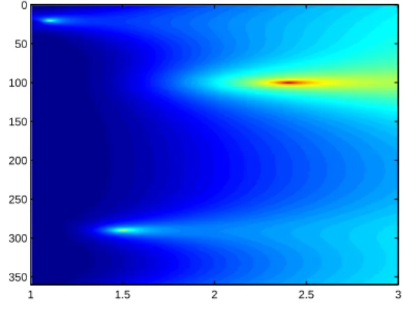
E(y) := Z _T 0 Z ∂Ω ∂pz ∂ν (x, t)vy(x, t) dσ(x) dt = c (y − z) · e 4π|z − y|3. (1.39) The projection on Σ of the location z can be obtained by taking the maximum of E(y) as y ∈ Σ. The third component of z can be obtained as the point on a line parallel to e where E(y) changes sign. This algorithm is parallel to the one developed in [25] for anomaly detection from electrical impedance boundary measurements.

1.4

Examples of Applications

1.4.1 Vibration Potential Tomography with FreeFem++

We present a test for iterative procedures proposed for the VPT reconstruction. The do-main Ω is the disk of radius 6 centered at the origin. Next to the boundary, that is, outside of a disk of radius 5, the conductivity is constant, equal to 1. In the region of the radius 5, the background conductivity is an oscillating function, sin

³

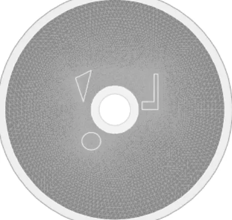
4px2_{+ y}2´_{+2. We introduced} three zones where the conductivity is notably different: An area with an irregular boundary where the conductivity is a piecewise constant function int (8/10 cos(4y) + 9/10) + 1/10, where int is the integer part function, a small stretched ellipse with constant conductivity 1/10, and an annulus where the conductivity increases rapidly (x + 2)2_{+ 0.1. The purpose} of choosing this pattern is to demonstrate that the reconstruction methods are very

Examples of Applications Section 1.4

effective for a large variety of conductivities. The conductivity distribution is presented on the Figure 1.1. The simulations are done using the partial differential equation solver FreeFem++ [15].

Figure 1.1: Conductivity Distribution.

Figure 1.2 shows the result of the reconstruction when perfect measurements (with ’infinite’ precisions) are available. We use two different Dirichlet boundary data, gx = 2 + x/6

and gy = 2 + y/6. In the first approach proposed in Section 1.3.1, this is implemented

by alternating the procedures with gx and gy. In the optimal control approach, this

corresponds to simply adding the contribution of both correctors. In both cases, the boundary data are positive, which implies the positivity of u in the domain Ω. The initial guess is depicted on the left: it is equal to 1 everywhere. The right picture represents the reconstructed conductivity after three iterations. A 7 digit accuracy in L2 _{norm and in}

L∞ _{norm is reached after five iterations.}

Figure 1.2: Perfect reconstruction test. From left to right, the initial guess, the reconstructed

conductivity after three iterations

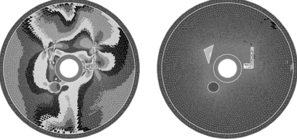
To document the effectiveness of our approach in the case of partial data, we perturb the measure data. We add 5% noise to the measured data, and we destroy the data on two elliptical subdomains, replacing it by 1. If we use solve iteratively, using alternatively the (perturbed) data corresponding to gx or gy, the algorithm cycles after fives iterations.

This is because we are trying to match mismatched data : the minimum corresponding to

g_x data is not the same as the one corresponding to g_y, because of the perturbations we applied to both data sets. The results are presented in Figure 1.3.

Figure 1.3: Perturbed reconstruction test. From left to right, the measured data for gx and gy,

and the reconstructed conductivity after five iterations

Note that the pattern is recognizable from the data E itself. This may be expected: thanks to De Giorgi-Nash estimates, the potential u is continuous, thus the data displays the discontinuities of γ. However, the value of γ cannot be read from the data. The local character of the minimization procedure is striking. The solution does not seem to be affected by a substantial loss of data. If we limit the minimization procedure to the area outside the elliptical subdomains instead of considering false data, the optimal control procedure converges to a non-zero minimum, which is due to the background noise. The reconstructed pattern is very similar to the one presented in Figure 1.3.

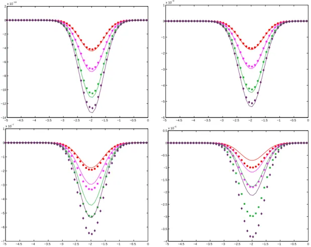
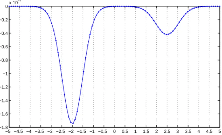
1.4.2 Magneto-Acoustic Tomographies with Incomplete Data

Suppose that the measurements of ∂pz/∂ν(x, t) are only done on a part Γ of the boundary

∂Ω. Suppose that T and Γ are such that they geometrically control Ω, which roughly means

that every geometrical optic ray, starting at any point x ∈ Ω, at time t = 0, hits Γ before time T at a nondiffractive point; see [10]. Let β ∈ C∞

0 (Ω) be a cutoff function such that

β(x) ≡ 1 in a subdomain Ω0 _{of Ω. Following [2], we construct by the geometrical control}

method a function ev(x, t) satisfying (1.25), the initial condition ev(x, 0) = β(x)vy(x, 0)

(vygiven by (1.28)), the boundary condition ev = 0 on ∂Ω\Γ, and the final conditions (1.26).

The reconstruction formulae (1.38) and (1.39) should be replaced by

cγ(z) ≈ −2cs|z − y| 2 r2 Z _T 0 Z Γ ∂pz ∂ν (x, t)ev(x, t) dσ(x) dt, (1.40) and _Z T 0 Z Γ ∂p_z ∂ν(x, t)ev(x, t) dσ(x) dt = c (y − z) · e 4π|z − y|3. (1.41)

1.5

Concluding Remarks

In this chapter, we have proposed two algorithms for solving the inverse problem in vibra-tion potential tomography. Both algorithms are based on transforming the conductivity

Concluding Remarks Section 1.5

equation into a nonlinear PDE. The first one follows from a perturbative approach while the second one follows an optimal control approach and can be applied to the case of incomplete data. It should be emphasized that from (1.4), an alternative way for solving the VPT problem is to first obtain j = γ|∇v| in each D and then to replace γ by j/|∇v| in the conductivity equation (1.1). This yields to exactly the same nonlinear problem as the one extensively investigated by Seo’s group for Magnetic Resonance Electrical Impedance Tomography (MREIT). An efficient algorithm for solving the inverse problem in MREIT is the so-called J−substitution algorithm. See for instance [22, 23]. We believe that if we restrict the resolution in the J−substitution algorithm to the size of D, it would lead to the same quality of conductivity images as the one provided in this chapter. However, the algorithms developed here for VPT are simpler and use only one current.

For magneto-acoustic tomography with magnetic induction, we provided explicit inversion formulae. Magneto-acoustic tomography transforms the inverse conductivity problem into a much simpler inverse source problem. Because of the acoustic boundary conditions, the spherical Radon inverse transform can not be applied. Our approach is to make an appropriate averaging of the measurements by using particular solutions to the wave equation. Our approach extends easily to the case where only a part of the boundary is accessible.

It is worth noticing that our approach for the magneto-acoustic tomography can be used in acoustic imaging (see [41] for a review of the current state-of-the-art of photo-acoustic imaging). We also intend to generalize our inversion formula to the case where the medium is acoustically inhomogeneous (contains small acoustical scatterers).

Chapter 2

Asymptotic Formulas for

Thermography Based Recovery of

Anomalies

2.1

Introduction

Medical thermal imaging has become a procedure of choice in the screening for breast, skin, or liver cancer [26]. It has the ability to identify various stages of disease development, and can pick up early stages which usually elude traditional anatomical examinations. Thermal imaging relies on the fact that chemical and blood vessel activity in pre-cancerous tissue and its surroundings are higher than in healthy tissue. Pre-cancerous and cancerous areas are characterized by heightened metabolism and require an abundant stream of nutrients to maintain growth. These extra nutrients are transported through various channels such as increased chemical activity, enhanced blood stream, and creation of new blood vessels (neoangiogenesis) [42]. This process results in a local increase in temperature.

Detection of these small temperature variations is made possible by state of the art imaging techniques. They involve ultra-sensitive thermal cameras and sophisticated soft-ware in detecting, analyzing, and producing high-resolution thermal images of vascular changes. More precisely, medical thermal imaging technique proceeds as follows: an infrared scanning device is used to convert infrared radiation emitted from the skin surface to electrical impulses. Those are then plotted on a color monitor. This map of body surface temperature is referred to as a thermogram. The spectrum of colors corresponds to a scale of infrared radiation emitted from the body surface. Since temperature distribution is highly isotropic in healthy tissue, subtle temperature anisotropies produce a clear imprint. See [1, 34].

Thermal imaging is a very reliable technology. In fact, clinical studies have shown that thermal imaging has an average sensitivity and specificity of 90% when applied to screening of breast tissue. As of today, an abnormal infrared image is the single most important

marker of high risk of onset breast cancer onset. Thermal imaging may also be used for different purposes such as

(i) assessing the extent of a previously diagnosed lesion;

(ii) localizing an abnormal area not previously identified, so further diagnostic tests can be performed;

(iii) detecting early lesions before they are clinically apparent;

(iv) guiding thermal ablation therapies.

In this chapter, we perform a quantitative study of temperature perturbation due to small thermal anomalies and we design algorithms for localizing these anomalies and estimating their size. We start from a realistic model in half space with convective boundary condition on the surface. It is noteworthy that our results can be applied to other types of thermography problems, such as the detection of buried objects in the underground. We seek to reconstruct only some rough feature of present anomalies. This partial reconstruction has the advantage to be stable against measurement noise and perturbation in geometry. Based on rigorously derived asymptotic estimates, we find an approximation formula that leads us to noniterative detection algorithms for finding dominant features of present anomalies.

We also consider in this chapter how to lay the mathematical background for ultrasonic temperature imaging. Ultrasonic temperature imaging is an essential tool for guiding medical devices in the course of thermal ablation therapy. It relies on the fact that sound speed in tissues depends on temperature. Thermal ablation therapy, such as focused ultrasound surgery, is a new way of destroying malignant tumors without damaging sur-rounding tissue. This technique consists of running the focused ultrasound surgery system at an initial, pre-ablative low intensity while using a diagnostic ultrasound imaging system to detect the associated localized temperature rise. This assumes that the temperature dependence of sound speed is known.

Let us now recall some previous results on anomaly detection by thermal imaging. In a recent paper [6], efficient noniterative algorithms for locating thermal anomalies from boundary measurements of temperature were introduced. The proposed reconstruction was based on a small volume assumption for the anomalies. The authors also assumed that the anomalies lay inside a bounded homogeneous domain, on whose boundary a heat flux was imposed. Resulting temperature was then measured on the same boundary. In another piece of work, Miller et al. [32] studied ultrasonic temperature imaging. Remarkably, their investigation lacks any mathematical analysis. We believe that a rigorous mathematical theory for the effects of thermal anomalies had to be investigated, since we want to perform a meticulate quantitative analysis. Ultimately this study should result in improving accuracy of lesion detection. In the following sections we will first present our novel mathematical analysis, we will then derive reconstruction algorithms. Numerical evidence validating these algorithms is presented in the last section of this chapter.