Development of a Spectroscopic Technique for Continuous
Online Monitoring of Oxygen and Site-Specific Nitrogen
Isotopic Composition of Atmospheric Nitrous Oxide
The MIT Faculty has made this article openly available. Please share
how this access benefits you. Your story matters.
Citation Harris, Eliza, David D. Nelson, William Olszewski, Mark Zahniser, Katherine E. Potter, Barry J. McManus, Andrew Whitehill, Ronald G. Prinn, and Shuhei Ono. “Development of a Spectroscopic Technique for Continuous Online Monitoring of Oxygen and Site-Specific
Nitrogen Isotopic Composition of Atmospheric Nitrous Oxide.” Analytical Chemistry 86, no. 3 (February 4, 2014): 1726–1734.
As Published http://dx.doi.org/10.1021/ac403606u
Publisher American Chemical Society (ACS)
Version Author's final manuscript
Citable link http://hdl.handle.net/1721.1/92437
Terms of Use Article is made available in accordance with the publisher's policy and may be subject to US copyright law. Please refer to the publisher's site for terms of use.
Development of a spectroscopic technique for
continuous online monitoring of oxygen and
site-specific nitrogen isotopic composition of
atmospheric nitrous oxide
Eliza Harris,
∗,†,‡David D. Nelson,
¶William Olsewski,
†Mark Zahniser,
¶Katherine
E. Potter,
†Barry J. McManus,
¶Andrew Whitehill,
†Ronald G. Prinn,
†and Shuhei
Ono
†Department of Earth, Atmospheric and Planetary Sciences, Massachusetts Institute of
Technology, 77 Massachusetts Ave, 02139 Cambridge USA, Laboratory for Air Pollution and
Environmental Technology, Swiss Federal Institute for Materials Science and Technology
(EMPA), Überlandstrasse 129, 8600 Dübendorf Switzerland, and Atmospheric and
Environmental Chemistry, Aerodyne Research Inc., 45 Manning Road, 01821 Billerica USA
E-mail: elizah@mit.edu
1
Abstract
2
Nitrous oxide is an important greenhouse gas and ozone depleting-substance. Its sources
3
are diffuse and poorly characterised, complicating efforts to understand anthropogenic impacts
4
and develop mitigation policies. Online, spectroscopic analysis of N2O isotopic composition 5
can provide continuous measurements at high time resolution, giving new insight into N2O 6
sources, sinks and chemistry. We present a new preconcentration unit, ‘Stheno II’, coupled
7
to a tunable infrared laser direct absorption spectroscopy (TILDAS) instrument, to measure
8
ambient-level variations in18O and site-specific15N N2O isotopic composition at remote sites 9
with a temporal resolution of <1 hour.
10
Trapping of N2O is quantitative up to a sample size of ∼4 L, with an optimal sample size of 11
1200-1800 mL at a sampling frequency of 28 minutes. Line shape variations with the partial
12
pressure of the major matrix gases N2/O2 and CO2 are measured, and show that characteri-13
sation of both pressure broadening and Dicke narrowing is necessary for an optimal spectral
14
fit. Partial pressure variations of CO2 and bath gas result in an linear isotopic measurement 15
offset of 2.6-6.0 ‰ mbar−1. Comparison of IR MS and TILDAS measurements shows that the
16
TILDAS technique is accurate and precise, and less susceptible to interferences than IR MS
17
measurements. Two weeks of measurements of N2O isotopic composition from Cambridge, 18
MA, in May 2013 are presented. The measurements show significant short-term variability in
19
N2O isotopic composition larger than the measurement precision, in response to meteorologi-20
cal parameters such as atmospheric pressure and temperature.
21
1
Introduction
22
Nitrous oxide (N2O) is a potent, long-lived greenhouse gas1 and, as a source of reactive nitrogen
23
to the stratosphere, the dominant contributor to catalytic ozone destruction in the 21st century.2
24
Since preindustrial times, N2O mixing ratio in the troposphere has increased from 270 ppb to the
25
current level of 324.2±0.1 ppb (2011) with an average growth rate of 0.2-0.3 % yr−1 over the
26
past decades.3–5 This increase has been attributed to anthropogenic perturbation of the nitrogen
27
cycle, in particular the application of inorganic fertilisers.5–8 The N2O budget, however, is poorly
28
constrained due to the high spatial and temporal variability of fluxes, which limits our ability to
29
develop targeted mitigation policies.9,10
30
14N14N18O) provide a useful constraint to quantify contributions from different N
2O sources*. The
32
major source of N2O is microbial production in natural and agricultural soils, by both nitrifying and
33
denitrifying bacteria. A number of studies have shown that the isotopic composition of N2O can
34
be used to distinguish between different microbial source pathways: The bulk15N composition of
35
N2O indicates the contribution of natural versus fertilized agricultural soil emissions,7,11,12 while
36
the site preference is independent of the reaction substrate and can be used to quantify different
mi-37
crobial processes, ie. nitrification versus denitrification.11–13Relationships between δ15Nα, δ15Nβ
38
and δ18O indicate the relative importance of N2O reduction to N2, and the oxygen isotopic
compo-39
sition also reflects the water in the environment where N2O was formed.14–17 In the troposphere,
40
N2O is stable and the major sink is transfer to stratosphere, where N2O is destroyed photolytically.
41
UV photolysis is shown to produce a strong enrichment in δ18O and δ15N of the residual N2O,
42
in particular, the central position15N (15Nα).18–20 This enrichment in15Nα can be a particularly
43
powerful tracer to quantify the magnitude of troposphere-stratosphere exchange, which is one of
44
the largest uncertainties in the global N2O budget.21 The δ15N and δ18O composition of ambient
45
N2O shows a definite decreasing trend over the past decades, reflecting the increasing contribution
46
of anthropogenic emissions, while observed trends in site preference remain inconclusive.5,7,22,23
47
Until recently, isotopic measurements of N2O have used the traditional technique of flask
sam-48
pling followed by laboratory-based isotope ratio-mass spectrometry (IR MS). While this technique
49
shows excellent precision for δ18O and δ15N, it is unsuitable for field deployment, and
continu-50
ous monitoring with high time resolution is technically challenging. In addition, site preference
51
measurements are complicated by scrambling in the ion source, non-mass-dependent oxygen
iso-52
tope composition, and mass interferences such as CO2.24–27Unlike IR MS, Tunable Infrared Laser
53
Direct Absorption Spectroscopy (TILDAS) measures fundamental rovibrational bands of nitrous
54
oxide isotopologues in the mid-infared regions at high precision, thus the technique can be used to
55
directly distinguish between15Nα and15Nβ. TILDAS techniques have been applied to a number
of isotopic systems such as CO2 and O3.28,29 Several recent studies have shown the potential of
57
TILDAS measurement coupled to a preconcentration unit for continuous, online measurement of
58
N2O isotopic composition.30–33
59
This study presents a new instrument that will be used to conduct online, real-time
measure-60
ments of N2O istopic composition at Mace Head Atmospheric Research Station, Ireland, as part
61
of the AGAGE network (http://agage.eas.gatech.edu). A cryogen-free preconcentration unit with
62
no chemical traps was developed to allow continuous, long-term monitoring at this remote site
63
with minimal maintainance. For the first time, isotopic reference gases labelled for both δ18O
64
and site-specific δ15N isotopic compositions were synthesised and measured with both IR MS and
65
TILDAS. A comprehensive treatment of matrix dependence for TILDAS results is presented, as
66
well as cross-calibration of site-specific isotope ratios against IR MS method, with an investigation
67
of scrambling corrections for IR MS. Ambient air measurements and TILDAS to IR MS
compar-68
ison show that TILDAS is both accurate and precise enough to observe ambient changes in δ18O,
69
15Nα and15Nβ of N
2O with a temporal resolution of 0.5-2 hours.
70
2
Materials and methods
71
2.1
Fully-automated cryogen-free N
2O preconcentration
72
For N2O preconcentration, we use a modified Medusa system34 known as ‘Stheno II’†. Medusa is
73
a fully-automated cryogen-free preconcentration unit coupled to GC/MS used to measure a
num-74
ber of CFCs and other non-CO2greenhouse gases at AGAGE stations;34a similar system has been
75
used previously to preconcentrate N2O for isotope measurements.32,35 The preconcentration
pro-76
cedure involves collecting N2O on a glass beads trap at approximately -156◦C and is described in
77
detail in Section S1 of the supplementary material. Our system differs from previous
preconcen-78
tration units used for spectroscopic measurements31–33in a number of ways, most notably, it uses
79
†The ‘Stheno II’ unit discussed here is a new unit, improving upon the principles used for the original ‘Stheno’
a glass beads trap rather than a HayeSep D trap to adsorb N2O, and CO2is not removed from the
80
sample air stream. These changes allow long-term operation with minimal maintenance. A basic
81
schematic of the preconcentration unit is shown in Figure 1 and an example of the
preconcentra-82
tion/trapping routine is presented in Figure 2.
83
2.2
Spectroscopic analysis of N
2O isotopic composition with TILDAS
84
Spectroscopic measurements are made with a dual-laser TILDAS instrument (Aerodyne Research
85
Inc), shown as the ‘laser cell’ in Figure 1. The instrument has two lasers tuned to 2188 and
86
2203 cm−1 to measure the four isotopocules of N2O, as shown in Figure 3. The spectroscopic
87
measurements are described in detail in Section S2 of the supplementary material. Measurements
88
are made at a pressure of 10 mbar with an N2O mixing ratio of 65 ppm and a CO2 mixing ratio
89
of 8% (see Section S2.4). Standards are run between every sample peak, as shown in Figure 2
90
(standards are discussed in Section S2.2). Following acquisition of the raw concentration data,
91
corrections are made to account for background, matrix effects, and calibration to the international
92
isotopic standard scale. The data analysis procedure and associated corrections are described in
93
detail in Section S2 of the supplementary material, and an example of the data analysis cycle is
94
shown in Figure S2.
95
2.3
Synthesis of standards by NH
4NO
3decomposition
96
A range of isotopic standards were synthesised via NH4NO3 decomposition to compare isotopic
97
measurements between IR MS and TILDAS. The synthesis is described in detail in Section S3 of
98
the supplementary material and only a brief description will be given here. NH4NO3with a range
99
of isotopic compositions was produced from recrystallizing stock NH4NO3with isotopic spikes of
100
Na15NO3, Na14NO3, 15NH4Cl and 14NH4Cl, as well as equilibration with H218O. The NH4NO3
101
2.4
Analysis of N
2O isotopic composition with isotope ratio-mass
spectrom-105
etry
106
Isotopic composition of N2O standard gases was measured with IR MS (Thermo Electron MAT
107
253). Pure N2O was used for analyses; gas chromatographic analysis with a thermal conductivity
108
detector (TCD) showed no detectable CO2 in N2O samples derived from NH4NO3
decomposi-109
tion (see Figure S6). Following Toyoda and Yoshida (1999), N2O+ (masses 44, 45 and 46) and
110
NO+(masses 30 and 31) ions were measured to determine position-specific15N substitutions.25,27
111
Analysis conditions are summarised in Table S3, and NO+ ion scrambling factors are discussed in
112
Section 3.1.2.
113
3
Results and discussion
114
3.1
Comparison of TILDAS and IR MS measurements
115
The five N2O standards synthesised by ammonium nitrate decomposition (Table S2) as well as
116
the two laboratory reference gases Ref I and Ref II were measured with IR MS and TILDAS
117
in order to cross-calibrate the TILDAS and IR MS measured isotopologue ratios and investigate
118
the accuracy of the two techniques considering IR MS scrambling factors and TILDAS matrix
119
corrections. The results are presented in Table S4 and summarised in Figure 4, and show very
120
good agreement between the IR MS and TILDAS for most samples. The instrument comparison
121
shows that TILDAS is able to provide accurate results across a wide range of N2O, CO2and bath
122
gas compositions and N2O isotopic compositions. TILDAS measurements at 23.5 and 40.5 ppm
123
N2O are not accurate: at [N2O] < approximately 45 ppm (at 0.010 atm, 1.7 × 10¹³ molec cm−3)
124
peaks are too small for fitting (<4% absorption depth) and results are not accurate. Sufficient N2O
125
should be trapped to achieve at least 45 ppm in the cell at 0.010 atm, corresponding to ∼1 L of air
126
at a typical atmospheric N2O mixing ratio of 327 ppb.
3.1.1 Matrix effects on spectroscopic line shape and measurement accuracy
128
The composition and pressure of the matrix has a significant effect on line shape, and thus on data
129
fits and measurement accuracy. Samples (trapped ambient and compressed air) and standards are
130
therefore matrix-matched as closely as possible. Measurement accuracy was tested across a range
131
of matrix compositions. A brief description of the results is given here; full details are presented
132
in Section S2.4 of the supplementary material. The primary matrix gas in the laser cell is zero air,
133
hereafter referred to as the ‘bath gas’; the N2:O2ratio of the bath gas does not have any significant
134
effect on the peak shape (Figure S4) or on measurement accuracy, as shown with measurements
135
of Ref II in a bath gas of 100% N2 and 100% O2 (Figure 4). The total pressure of bath gas, on
136
the other hand, has a significant effect on the results, affecting measured isotopic composition
137
by ∼2.6-6‰ mbar−1. The measurement pressure for standards is therefore regulated by the bulk
138
expansion volume pressure (∼750 mbar; Section S2.2) in the ‘standard reservoirs’ shown in Figure
139
1, while the pressure for trapped sample measurements is controlled to within ±2% by the length
140
of the flush into the cell (∼90 seconds; Section S1 and Figure 2). An empirical pressure correction
141
is applied to account for the small differences in pressure that remain (±0.3 mbar; Section S2.3).
142
The CO2partial pressure affects the measurement accuracy with the same order of magnitude
143
as the bath gas pressure (∼2.6-4‰ mbar−1; Table S1 and Figure S3), however it cannot be
con-144
trolled in trapped samples as the ambient pressure of CO2 shows significant temporal variation,
145
for example >10% at Mace Head Station.37,38 A pressure correction is therefore also applied to
146
account for differences in CO2 partial pressure, in addition to the pressure correction for bath gas
147
pressure (Section S2.3). The empirically-determined pressure dependencies are highly linear over
148
the range of interest and show less than 5% change over longer time periods (Section S2.4, Table
149
S1); therefore they introduce <0.05‰ error under normal measurement conditions. Ref II was
150
measured in a matrix with 14% CO2 equivalent to an ambient mixing ratio of 700 ppm,
requir-151
ing pressure corrections of -1.73±0.09‰, 1.67±0.08‰ and -2.56±0.13‰ for δ15Nα, δ15Nβ and
The pressure dependence of isotopic measurements is most likely caused by changes in peak
155
shape and broadening in response to different matrix gases. Peak width in the TDL Wintel software
156
used for spectroscopic data analysis (Aerodyne Research, Inc.) is described by an approximated
157
Voigt profile, which can be deconvolved into contributions from the gaussian Doppler line shape
158
function and the Lorentz line shape function due to pressure broadening.39 Both Gaussian and
159
Lorentzian line widths were estimated as a function of pressure (see Figure S7) by fitting measured
160
spectra to a Voigt profile to find an optimum fit and exact width. The extent of pressure broadening
161
and Dicke narrowing were estimated for comparison with literature values from the HITRAN
162
database.40,41The measurements and calculations are presented in Section S4 of the supplementary
163
material; the results will be described here. ‡
164
The parameters describing peak shape are summarised in Table 1. For all four N2O peaks, it
165
can be seen that the derived air broadening coefficients are consistently higher than given in the
166
HITRAN database: ∼2% for14N14N16O and14N14N16O (within the uncertainty of HITRAN data),
167
6% for 15N14N16O and 8% for 14N14N18O (significantly different to HITRAN data42–44). The
168
HITRAN values for N2O are measured at high pressures (>0.09 atm,42,43) relative to the pressures
169
at which these measurements were made (∼0.01 atm); more importantly, while the HITRAN line
170
widths and strengths are taken from measurements of both14N14N16O and the minor isotopes, the
171
HITRAN broadening coefficients are taken from measurements of only14N14N16O.42–44
172
Although the estimate of Dicke-narrowing factor45(Eq. S7) is based only on a parameterisation
173
and the effects of narrowing are expected to be largest at ∼0.06-0.07 atm,46the results clearly show
174
that there is significant narrowing at the low pressures used in the TILDAS cell. At measurement
175
pressure of 10 mbar (0.01 atm), the Doppler width (2-2.3 cm−1for the four N2O peaks; see Figure
176
S7) contributes a large part of the total Voigt line width (2.4-2.8 cm−1). Dicke narrowing has a
177
significant impact on the Doppler width and the fit, accounting for ∼50% of peak width change
178
with pressure, and thus it is an important feature needed to gain accurate and precise results. We
179
have implemented this narrowing into our fits and find a significant improvment in precision of
180
repeated measurements on the order of 3-4×; eg. precision on δ15Nα is 0.25-0.4‰ without the
181
‘Dicke factor’ and improves to 0.07-0.15‰ when the ‘Dicke factor’ is included in the fit.
182
3.1.2 Scrambling in the ion source in IR MS analyses
183
Site-specific N2O isotopic composition is measured indirectly in the IR MS, by monitoring the
184
isotopic composition of N2O+ ions (m/z = 44, 45, 46) and NO+ ions (m/z = 30, 31). 15NO+ ions
185
result primarily from fragmentation of 14N15NO, thus the site-specific isotopic composition can
186
be inferred.24–26 This method is complicated by scrambling in the ion source, which means that
187
∼8% of15NO+is actually derived from15N14NO, and also replies on the assumption that the
oxy-188
gen isotopic composition is mass-dependent.27This assumption is the reason why the site-specific
189
isotopic composition for 448-H sample, which is strongly enriched in18O, is poorly characterised
190
with IR MS measurements, as shown in Figure 4: the directly-measured value of δ18O (mass 46) is
191
used to infer δ17O according to a mass-dependent relationship (Eq. 9 in the supplementary
mate-192
rial). The inferred δ17O is then used to iteratively calculate site-specific15N isotopic composition
193
from masses 45 (15N14N16O+, 14N15N16O+ and 14N14N17O+) and 31 (15N16O+ and 14N17O+)
194
(see Eqs. 10, 11 and 13 in the supplementary material). Thus, if the sample oxygen isotopic
com-195
position is not mass-dependent, the calculated values of δ17O and thus site-specific N2O isotopic
196
composition are incorrect. In contrast, TILDAS is able to accurately measure site-specific 15N
197
substitutions across a large range of δ17O, δ18O and ∆17O values.
198
Scrambling in the ion source was considered by comparing the measured isotopic composition
199
of the standards (not including 448-H), which have site preference values ranging from -1.76 to
200
+15.09‰, between the IR MS and the TILDAS. Although the TILDAS values have an associated
201
measurement error, the site-specific15N substitutions are directly measured, thus there is no
sys-202
tematic relationship between site preference and error. Averaging across all the seven standards
203
can therefore give an accurate view of IR MS measurement quality without a bias from TILDAS
5. Two possible scrambling models are considered:
207
• ‘one factor’ scrambling, with equal yield of15NO+from15N14NO and14NO+from14N15NO
208
described by a single scrambling factor ’γ’, ie. γ of 0.08 means 8% of15NO+is derived from
209
15N14NO and similarly for14NO+
210
• ‘two factor’ scrambling, where the scrambling of14N15NO (γα) is not equal to the
scram-211
bling of 15N14NO (γβ) (differences due to other isotopic substitution possibilities are not
212
accounted for, eg. clumped,17O,18O)
213
More complex scrambling models have also been considered27 however the number of standards
214
in this study is too small to consider the accuracy of models with a larger number of variables.
215
In agreement with the results of Westley et al.,27scrambling is more complex than a one-factor
216
scrambling model can account for: The IR MS and TILDAS results never agree within the
mea-217
surement error (Figure S8) with the one factor correction. Overall, best agreement is seen for
218
one factor scrambling with γ = 8%, consistent with results obtained using similar source
condi-219
tions.24,25,27 However, for calculation of δ15Nα, best agreement is obtained with a scrambling
220
factor of 9%, highlighting the limitations of the one-factor model.
221
The results from comparison of IR MS and TILDAS with two-factor scrambling show ∼0.05‰
222
improvement in accuracy for the IR MS measurement compared to one-factor scrambling. The
ac-223
curacy of results is much more sensitive to the scrambling of14N15NO (γα) than 15N14NO (γβ).
224
From consideration of δ15Nα, δ15Nβ and site preference, it is clear that the optimal value of
225
γα is 8-9%, in agreement with previous studies,24,25,27 while the optimal value of γβ is clearly
226
lower - between 2 and 4%. This value is much lower than reported by previous studies (eg.
sin-227
gle factor of 8.5% from Brenninkmeijer et al. 2009;24 γβ of ∼9% from Westley et al. 200727).
228
This study presents the widest range of isotopic references gases yet considered and does not rely
229
on primary calibration through techniques such as NH4NO3 decomposition or enriched gas
mix-230
ing,24,25,27,47 which give uncertainties of >0.2-0.3‰ in site preference, but instead presents the
site preference values in previous studies may not have been high enough to fully assess the
op-233
timum value of γβ, considering that the calculated site preference is much less sensitive to the
234
chosen value of γβ than the value of γα.
235
Even with the optimised two-factor scrambling model, correcting for scrambling in the ion
236
source introduces an error larger than the combined IR MS and TILDAS measurement uncertainty
237
for both δ15Nα and site preference (δ15Nβ is accurate to within the measurement uncertainty).
238
The error that is introduced depends on the site preference value of the N2O being considered,
239
therefore both measurement precision and accuracy are affected. This limits the potential of IR
240
MS measurements for high-precision monitoring of site-specific N2O isotope ratios in lab and
241
field studies, particularly at remote background sites like Mace Head where relevant changes in
242
isotopic composition are very small.
243
3.2
Isotopic measurements in preconcentrated samples
244
3.2.1 Trapping efficiency: Trace gas recovery
245
Quantitative recovery of N2O following trapping is critically important to prevent introduction of
246
isotope fractionation by absorption/desorption processes.48,49 Unlike previous instruments,31–33
247
the Stheno II preconcentration unit (and the predecessor Stheno I35) uses a glass beads trap instead
248
of the stronger HayeSep D adsorbent. The major advantage of the glass beads trap is that no N2/O2
249
is trapped from the air; thus, the bath gas is added as a flush with a known composition, making the
250
pressure and matrix easier to accurately control. The range over which glass beads can efficiently
251
trap N2O was investigated by trapping increasing amounts of sample and comparing the measured
252
and expected N2O and CO2 concentrations, as shown in Figure 6. N2O is efficiently trapped
253
when the sample volume is <4 L; CO2is efficiently trapped until ∼2 L. It is desirable to use the
254
minimum trapped volume, to conserve sample when measuring flask samples and to achieve the
255
range, N2O recovery is >99% and therefore the fractionation introduced by trapping is negligible.
259
3.2.2 Measurements of N2O isotopic composition in ambient samples from Cambridge,
260
Massachusetts
261
N2O isotopic composition was measured continuously from MIT’s ‘Green Building’ for two weeks
262
between March 3-16, 2013. The sampling inlet was located on the roof of the 18-story (95 m)
263
building and connected to sampling pumps (see Figure 1) with >50 m of Synflex 1300 tubing
264
(Eaton Corporation, USA). Samples were measured every 28 minutes, and for every 5-10 ambient
265
air samples, one compressed air sample (Medical grade, Airgas Inc.) was measured to monitor
266
trapping efficiency and precision. The compressed air measurements and precision histograms
267
are shown in Figure S9; the capabilities of the instrument are summarised in Table 2. Precision
268
is better for δ15N than δ18O due to the relatively small absorption depth of the14N14N18O peak
269
(Figure 3).
270
Ambient air measurements over the 13-day period are shown in Figure 7. The scatter in
am-271
bient air measurements (‘true’ variability + measurement error; bars in Figure 7 histograms) was
272
compared to the scatter in compressed air measurements (measurement error only; smooth line
273
in Figure 7 histograms), to determine if the instrument precision is sufficient to see changes in
274
isotopic composition of ambient air. δ18O values show a large amount of true variability over the
275
measurement period, thus although precision is lowest for this isotopocule, the precision is
suffi-276
cient to observe ambient variations for both single measurement and four-point moving average.
277
For δ15Nβ, there is some true variability outside the measurement error with single measurements,
278
although the difference between frequency distributions is much clearer for the four-point average
279
data. The true variability is smaller than the measurement error of single measurements for both
280
δ15Nα and δ15Nbulk; true variability of these isotopocules can only be resolved using the four-point
281
moving average.
282
The isotopic measurements were compared to weather variables to examine causes of
summarised in Table S5 in the supplementary material. All four isotopomers show a significant
285
relationship to pressure; a positive correlation for δ18O and a negative correlation for all15N
iso-286
topomers. This correlation may relate to exchange of free tropospheric air. Relative humidity
287
showed a significant correlation with all isotopocules except δ15Nα. It is possible that this
re-288
lates to partitioning between different microbial pathways. Wind direction showed a significant
289
relationship to δ15Nβ, with slightly isotopically heavier N
2O originating from the continent and
290
isotopically light N2O from the marine sector. A full investigation of the relationship between
291
meteorological variables and measured isotopic composition is beyond the scope of this study and
292
will be discussed in a later publication.
293
4
Conclusions
294
Measurement of N2O isotopic composition has traditionally involved the collection of flask
sam-295
ples, which are then purified and measured with IR MS in a laboratory. While this technique has
296
yielded interesting results, potential for investigations of seasonal cycles or changes in sources
re-297
lated to meteorology is limited by the feasible number and temporal resolution of samples. Using
298
preconcentration without CO2 removal followed by TILDAS, we have obtained sufficient
preci-299
sion with a four-point moving average of 28-minute measurements to observe ambient remote-site
300
changes in all the isotopocules of N2O, and we have demonstrated accuracy across a wide range
301
of isotopic composition and site preference values. The ‘Stheno II’ instrument is automated and
302
remotely operated, and uses very few consumables, to be well-suited for remote deployment at
303
sites such as Mace Head Atmospheric Research Station.
304
The time series in Figure 7 shows that there is significant variability in N2O isotopic
composi-305
tion on very short time scales. The data shows decoupling between15N and18O content of N2O.
306
Variability in δ18O is larger than variability in δ15Nβ, which is in turn greater than variability in
307
combination with inverse modelling and analysis of other trace gases and meteorological variables,
310
the results can be used to provide new insight into N2O variability.
311
Acknowledgments
312
We thank S. Toyoda and N. Yoshida at Tokyo Tech for calibration of reference N2O, and S.
313
O’Doherty, D. Young and G. Spain for helpful suggestions regarding field deployment. We
ac-314
knowledge NSF Grant #0959280 “MRI-R2: Development and Deployment of Automated
Contin-315
uous Wave Quantum Cascade Laser Instruments for On-Site Monitoring of the Four Isotpomers of
316
Nitrous Oxide” for supporting this work.
Figures and Tables
318 Nafion V3 AACA ZAThr ee spar e inlets Two-position valve Pressure sensor Flow controller 1 Diaphragmpump (DP1) Trappingoutlet control
Flow controller 2
V1 V4 V5 ZA flushsource
Diaphragm
pump (DP2) reservoirsStandard
Pressure regulators Standard #1 Standard #2 Pressure sensor ZA flush source V14 V13 V12 V11 V10 V9 V8 V7 V6 Pressure sensor 76 m path laser cell Scroll pump V15 Standard manifold for introduction by bulk expansion Inlet 20 m t ow er Vent Vent Inlet gas Flow meter Flow meter Pressure gauge Back pressure regulator DP3 DP4 Cryo-trap T1
Figure 1: Schematic of the modified Medusa system ‘Stheno II’, developed for preconcentration of N2O without the use of chemical traps or liquid nitrogen. ‘V’ specifies a valve, ‘T’ is a trap, ‘DP’ specifies a diaphragm pump, ‘ZA’ = zero air, ‘AA’ = ambient air, ‘CA’ = compressed air. The instrument is shown with valve #3 in the ‘trapping’ position. The system is described in detail in Section S1 of the supplementary material.
-180 -170 -160 -150
Cold head temperature (
˚C) -200 -100 0 100 Trap temperature ( ˚C) 0 250 500
Trap flow rate (sccm)
0
Flushing flow rate (sccm)
24.5 25 25.5 Cell temperature (˚C) 0 25 50 Cell pressure (mbar)
5 10 15 20 25 30 35 0 2 [N2 O] (molec cm -3) 0 4 5 [CO 2] (molec cm -3 ) 3 6 x 10¹³ 1.5 0.5 1 1 2 3 x 10¹⁶ Time (minutes) Desorption Baking Trapping Trapping Flush sample into cell
Cleaning trap
Std Sam Std
Fill/pump cycles
Std Sam Std
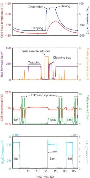
Figure 2: Trapping routine used for N2O preconcentration on a liquid-nitrogen free glass beads trap, coupled to TILDAS isotope measurement. The first panel shows the cold head (red) and trap (blue) temperatures. The second panel shows the flow rate through the trap (purple; both flush and sample) and the flushing flow used to push the sample into the laser cell (orange; spikes are due to multiport valve switching and do not affect measurement). The third panel shows the pressure (green) and temperature (red) in the laser measurement; the periods where the cell is cleaned are indicated, and ‘Std’ refers to a standard while ‘Sam’ refers to a sample. The fourth panel shows the concentration (molec cm−3) of N2O (major isotope; blue) and CO2 (grey) measured in the laser cell.
1.0 0.98 0.94 0.96 446 546 456 CO2 Tr ansmission 2187.85 2187.95 2188.05 Measurement Fit Wavelength (cm-1) 1.0 0.98 0.90 0.96 0.92 0.94 2203.25 2203.35 2203.15 446 546 456 448 CO CO 2 2203.45 Laser 1 Laser 2
Figure 3: Measured (blue dots) and fitted (red line) spectra for Laser 1 (2188 cm−1) and Laser 2 (2203 cm−1). The peaks used for isotope measurements are circled with a gray dashed line. Measurement conditions: 8.9% CO2, 69.5 ppm N2O in synthetic air, P = 11.9 mbar, T = 298 K, path = 76 m. The HITRAN lines and simulated (≡ expected) spectra for the two lasers are shown in Figure S1 for comparison with the measured and fitted spectra.
50 70 130 110 90 50 70 90 110 130 10 0 -10 -20 -30 30 20 10 0 -10 -20 -30 20 30 10 0 -10 -20 -30 30 20 10 0 -10 -20 -30 20 30 10 0 -10 -20 30 20 10 0 -10 -20 20 30 IR MS ( ‰) IR MS ( ‰) TILDAS (‰)
δ
18O
δ
15N
bulkδ
15N
αδ
15N
β Mean: 0.04±0.22 Mean: 0.09±0.21 Mean: 0.09±0.14 Mean: 0.08±0.17 150 150 38 42 40 38 40 42 ‘Normal’ samples: ~65 ppm N2O, 8% CO2 in synthetic air 18O enriched 23.5 ppm N2O 40.5 ppm N2O 14% CO2 Bath gas = N2 Bath gas = O2 TILDAS (‰) TILD AS - IR-MS ( ‰) 0 2 -2 TILD AS - IR MS ( ‰) 6 2 -2 0 2 -6 -3 -4 0 4 TILDAS (‰)Figure 4: Comparison of N2O isotope ratios measured with IR MS (y-axis) and TILDAS (x-axis) for the four isotopocules of N2O. The offsets between the two techniques (TILDAS - IR MS) are shown under each plot. The exact values can be seen in supplementary Table S4. The majority of samples were measured in the normal matrix (blue squares) but accuracy was tested across several matrix pertubations: low N2O mixing ratio (yellow open and green filled circles), high CO2mixing ratio (red squares), and N2 and O2 bath gases (purple star and grey diamonds respectively). 18O enriched samples are indicated with open blue stars due to importance of 18O composition when calculating site-specific15N composition of N2O with IR MS.
γ
βδ
15N
α 0.05 0.1 0.15 0.2 0 0.05 0.1 0.15 0.2 0.05 0.1 0.15 0.2 0 0.05 0.1 0.15 0.2 0.05 0.1 0.15 0.2 0 0.05 0.1 0.15 0.2γ
βγ
βγ
αδ
15N
βSite preference
Average accuracy of IR MS result (‰)
2 1.5 1 0.65 0.35 0.15
Figure 5: Absolute accuracy of site-specific N2O isotopic measurements made with IR MS (defined as | (δ15Nα)
IRMS− (δ15Nα)TILDAS | averaged across the six N2O standards, and similarly for
δ15Nβ and site preference). Two-factor scrambling results are shown with the contour plot: γα (x-axis) shows the scrambling of14N15NO, and γβ (y-axis) shows the scrambling of15N14NO. The lowest point of the contour plot shows the optimum scrambling factors. The dashed line indicates where both factors are equal, which is equivalent to the one-factor scrambling model. The star indicates where the deviation for the one factor model is at a minimum (see Figure S8 for a full plot of one-factor scrambling results).
Measured Expected N2O CO2 [N2 O ] (ppm) or [ CO 2 ] (ppt) 400 300 100 200 1000 2000 3000 4000 5000 0 Volume trapped (mL)
Minimum [N2O] for isotope measurements
Optimal trapping range
Figure 6: Measured (circles) and expected (dotted lines) mixing ratios of N2O and CO2 as the volume of air trapped is increased from 400 to 5200 mL. The expected mixing ratio is curved with respect to volume trapped as the cell pressure also increases when a greater quantity of gas is trapped. The dashed line shows the minimum N2O mixing ratio (at 10 mbar total cell pressure) required for accurate isotope analysis. Testing was performed with a flow rate of 370 sccm; further tests showed trapping efficiency is not affected by trapping flow rate up to 500 sccm.
36 38 40 42 14.5 15 15.5 16 16.5 04 05 06 07 08 09 10 11 12 13 14 15 16 −4 −3.5 −3 −2.5 5.5 6 6.5 7 −2 0 2 4 0 50 100 150 200 −0.5 0 0.5 1 0 20 40 60 80 −0.5 0 0.5 1 0 20 40 60 80 −0.5 0 0.5 1 0 20 40 60 80 100 ∆(δ18O) ∆(δ15N bulk) ∆(δ15Nα) ∆(δ15Nβ) δ 18 O δ 15 N bulk δ 15 N α δ 15 N β
Date (analyses started May 3rd at 08:22:55)
Fr equenc y Fr equenc y Fr equenc y Fr equenc y −2 0 2 4 0 40 80 120 0 0.5 0 40 80 120 0 0.5 0 20 40 60 80 100 −0.5 0 0.5 1 0 40 80 120 −0.5 −0.5 ∆(δ18O) ∆(δ15N bulk) ∆(δ15Nα) ∆(δ15Nβ)
Single measurements Four-point average
Figure 7: N2O isotope ratios from repeated measurements of ambient air in Cambridge, MA. Left-hand panels show measured isotopic composition with time: points are individual measurements, and thick lines show the 4-point moving average. The thickness of the line corresponds to the 1σ error determined from repeated measurements of compressed air: 0.16, 0.08, 0.085 and 0.095‰ for δ18O, δ15Nbulk, δ15Nα and δ15Nβ respectively. Right-hand panels show the frequency distribution of deviations from the mean value in permil for single measurements and for four-point moving averages; ie. ∆(δ18O) = δ18Ox - mean(δ18O). Bars show the measured frequency distribution for ambient air measurements, while lines show the expected Gaussian distribution based on random error only, determined from repeated measurements of compressed air.
Table 1: Air-, self- and CO2-broadening coefficients in cm−1atm−1 for N2O and CO2peaks mea-sured by varying air (bath gas) pressure between 0.0076 and 0.0113 atm and CO2pressure between 0.0005 and 0.0013 atm (see Figure S7). N2O pressure was 5×10⁻⁷ atm, thus self-broadening of N2O was negligible during measurements. Molecule: numbers in brackets refer to the HITRAN identification number of the molecule. Peak positions are cm−1.
Lorentz width Doppler width
Molecule Peak position γair γself γCO2 βair βCO2
HITRAN This study HITRAN This study
14N14N16O (41) 2188.0448 0.0838 0.0858 0.110 0.0268 3.70 9.73 14N15N16O (42) 2187.9432 0.0798 0.0812 0.104 0.0409 4.05 16.56 15N14N16O (43) 2187.8460 0.0774 0.0837 0.101 0.0408 5.53 14.97 14N14N18O (44) 2203.2808 0.0774 0.0818 0.101 0.0286 4.84 11.91 319 320
Table 2: Summary of the precision attainable with TILDAS measurements of N2O isotopic com-position. ‘Precision’ is the 1σ standard deviation of repeated measurements of compressed air.
naveraged is the amount of measurements that need to be averaged to achieve a certain precision.
δ18O δ15Nα δ15Nβ δ15Nbulk
Precision (‰), 28 min time resolution 0.32 0.17 0.19 0.16
naveraged for <0.2‰ precision 3 No averaging required
Temporal resolution (hours) 1.4 0.5 0.5 0.5
naveraged for <0.1‰ precision 11 3 4 3
References
321
(1) IPCC, In Contribution of Working Group I to the Fourth Assessment Report of the
Intergov-322
ernmental Panel on Climate Change; Solomon, S., Qin, D., Manning, M., Chen, Z.,
Mar-323
quis, M., Averyt, K. B., Tignor, M., Miller, H. L., Eds.; Cambridge University Press, 2007.
324
(2) Ravishankara, A. R.; Daniel, J. S.; Portmann, R. W. Science 2009, 326, 123–125.
325
(3) Khalil, M. a. K.; Rasmussen, R. a.; Shearer, M. J. Chemosphere 2002, 47, 807–21.
326
(4) Park, S.; Croteau, P.; Boering, K. A.; Etheridge, D. M.; Ferretti, D.; Fraser, P. J.; Kim, K.
327
. R.; Krummel, P. B.; Langenfelds, R. L.; van Ommen, T. D.; Steele, L. P.; Trudinger, C. M.
328
Nature Geoscience2012, 5, 261–265.
329
(5) Toyoda, S.; Kuroki, N.; Yoshida, N.; Ishijima, K.; Tohjima, Y.; Machida, T. Journal of
Geo-330
physical Research - Atmospheres2013, 118, 1–13.
331
(6) Sowers, T.; Rodebaugh, A.; Yoshida, N.; Toyoda, S. Global Biogeochem. Cycles 2002, 16,
332
1129.
333
(7) Rockmann, T.; Kaiser, J.; Brenninkmeijer, C. A. M. Atmospheric Chemistry and Physics
334
2003, 3, 315–323.
335
(8) Wolf, B.; Zheng, X.; Brüggemann, N.; Chen, W.; Dannenmann, M.; Han, X.; Sutton, M. a.;
336
Wu, H.; Yao, Z.; Butterbach-Bahl, K. Nature 2010, 464, 881–4.
337
(9) Nishina, K.; Akiyama, H.; Nishimura, S.; Sudo, S.; Yagi, K. J. Geophys. Res. 2012, 117,
338
G04008–.
339
(10) Cavigelli, M. A.; Grosso, S. J. D.; Liebig, M. A.; Snyder, C. S.; Fixen, P. E.; Venterea, R. T.;
340
Leytem, A. B.; McLain, J. E.; Watts, D. B. Frontiers in Ecology and the Environment 2012,
(11) Park, S.; Perez, T.; Boering, K. A.; Trumbore, S. E.; Gil, J.; Marquina, S.; Tyler, S. C. Global
343
Biogeochemical Cycles2011, 25, GB1001.
344
(12) Perez, T.; Trumbore, S. E.; Tyler, S. C.; Matson, P. A.; Ortiz-Monasterio, I.; Rahn, T.;
Grif-345
fith, D. W. T. Journal of Geophysical Research - Atmospheres 2001, 106, 9869–9878.
346
(13) Sutka, R. L.; Ostrom, N. E.; Ostrom, P. H.; Breznak, J. A.; Gandhi, H.; Pitt, A. J.; Li, F.
347
Applied and Environmental Microbiology2006, 72, 638–644.
348
(14) Yoshinari, T.; Wahlen, M. Nature 1985, 317, 349–350.
349
(15) Wahlen, M.; Yoshinari, T. Nature 1985, 313, 780–782.
350
(16) Ostrom, N. E.; Pitt, A.; Sutka, R.; Ostrom, P. H.; Grandy, A. S.; Huizinga, K. M.;
Robert-351
son, G. P. Journal of Geophysical Research-biogeosciences 2007, 112, G02005.
352
(17) Snider, D. M.; Venkiteswaran, J. J.; Schiff, S. L.; Spoelstra, J. GLOBAL CHANGE BIOLOGY
353
2012, 18, 356–370.
354
(18) Rahn, T.; Zhang, H.; Wahlen, M.; Blake, G. A. Geophysical Research Letters 1998, 25,
355
4489–4492.
356
(19) Rockmann, T.; Kaiser, J.; Brenninkmeijer, C. A. M.; Crowley, J. N.; Borchers, R.;
357
Brand, W. A.; Crutzen, P. J. Journal of Geophysical Research 2001, 106, 10403–10410.
358
(20) Kaiser, J.; Engel, A.; Borchers, R.; Rockmann, T. Atmospheric Chemistry and Physics 2006,
359
6, 3535–3556.
360
(21) Park, S. Y.; Atlas, E. L.; Boering, K. A. Journal of Geophysical Research - Atmospheres
361
2004, 109.
362
(22) Rahn, T.; Wahlen, M. Global Biogeochem. Cycles 2000, 14, 537–543.
363
(24) Brenninkmeijer, C. A. M.; Röckmann, T. Rapid Communications in Mass Spectrometry 1999,
365
13, 2028–2033.
366
(25) Toyoda, S.; Yoshida, N. Analytical Chemistry 1999, 71, 4711–4718.
367
(26) Kaiser, J.; Röckmann, T.; Brenninkmeijer, C. A. M. Journal of Geophysical Research 2003,
368
108, 4476.
369
(27) Westley, M.; Popp, B. N.; Rust, T. M. Rapid Communications in Mass Spectrometry 2007,
370
21, 391–405.
371
(28) Weidmann, D.; Wysocki, G.; Oppenheimer, C.; Tittel, F. K. Applied Physics B-lasers and
372
Optics2005, 80, 255–260.
373
(29) Janssen, C.; Tuzson, B. Applied Physics B-lasers and Optics 2006, 82, 487–494.
374
(30) Uehara, K.; Yamamoto, K.; Kikugawa, T.; Yoshida, N. Spectrochimica Acta Part A:
Molecu-375
lar and Biomolecular Spectroscopy2003, 59, 957–962.
376
(31) Mohn, J.; Guggenheim, C.; Tuzson, B.; Vollmer, M. K.; Toyoda, S.; Yoshida, N.;
Emmeneg-377
ger, L. Atmospheric Measurement Techniques 2010, 3, 609–618.
378
(32) Mohn, J.; Tuzson, B.; Manninen, A.; Yoshida, N.; Toyoda, S.; Brand, W. A.; Emmenegger, L.
379
Atmospheric Measurement Techniques2012, 5, 1601–1609.
380
(33) Köster, J. R.; Well, R.; Tuzson, B.; Bol, R.; Dittert, K.; Giesemann, A.; Emmenegger, L.;
381
Manninen, A.; Cárdenas, L.; Mohn, J. Rapid communications in mass spectrometry : RCM
382
2013, 27, 216–22.
383
(34) Miller, B. R.; Weiss, R. F.; Salameh, P. K.; Tanhua, T.; Greally, B. R.; Simmonds, P. G.;
384
Mühle, J. Analytical Chemistry 2008, 80, 1536–1545.
(36) Potter, K. Nitrous oxide (N2O) isotopic composition in the troposphere: instrumentation,
ob-388
servations at Mace Head, Ireland, and regional modeling. PhD Thesis, Massachusetts Institute
389
of Technology, 2011.
390
(37) Sirignano, C.; Neubert, R. E. M.; Rödenbeck, C.; Meijer, H. a. J. Atmospheric Chemistry and
391
Physics2010, 10, 1599–1615.
392
(38) Derwent, R.; Ryall, D.; Manning, A.; Simmonds, P.; O’Doherty, S.; Biraud, S.; Ciais, P.;
393
Ramonet, M.; Jennings, S. Atmospheric Environment 2002, 36, 2799–2807.
394
(39) McManus, J. B.; Nelson, D. D.; Shorter, J.; Zahniser, M.; Mueller, A.; Bonetti, Y.; Beck, M.;
395
Hofstetter, D.; Faist, J. Proceedings of SPIE 2002, 4817, 22–33.
396
(40) Rothman, L. et al. Journal of Quantitative Spectroscopy and Radiative Transfer 2009, 110,
397
533–572.
398
(41) Rothman, L. S.; Gamache, R. R.; Goldman, A.; Brown, L. R.; Toth, R. a.; Pickett, H. M.;
399
Poynter, R. L.; Flaud, J. M.; Camy-Peyret, C.; Barbe, A.; Husson, N.; Rinsland, C. P.;
400
Smith, M. a. Applied Optics 1987, 26, 4058–97.
401
(42) Nemtchinov, V.; Sun, C.; Varanasi, P. Journal of Quantitative Spectroscopy and Radiative
402
Transfer2004, 83, 267–284.
403
(43) Toth, R. A. Journal of Quantitative Spectroscopy and Radiative Transfer 2000, 66, 285–304.
404
(44) Lacome, N.; Levy, A.; Guelachvili, G. Applied optics 1984, 23, 425–35.
405
(45) Demtroeder, W. Laser Spectroscopy: Basic Prin, 4th ed.; Springer-Verlag: Berlin,
Heidel-406
berg, 2008; p 473.
407
(46) Tasinato, N.; Duxbury, G.; Langford, N.; Hay, K. G. The Journal of chemical physics 2010,
408
132, 044316.
(47) Kaiser, J.; Rockmann, T.; Brenninkmeijer, C. A. M.; Crutzen, P. J. Atmospheric Chemistry
410
and Physics2003, 3, 303–313.
411
(48) Bertolini, T.; Rubino, M.; Lubritto, C.; D’Onofrio, A.; Marzaioli, F.; Passariello, I.; Terrasi, F.
412
Journal of Mass Spectrometry2005, 40, 1104–8.
413
(49) Archbold, M. E.; Redeker, K. R.; Davis, S.; Elliot, T.; Kalin, R. M. Rapid communications in
414
mass spectrometry2005, 19, 337–42.
Supplementary Information: Development of a
spectroscopic technique for continuous online
monitoring of oxygen and site-specific nitrogen
isotopic composition of atmospheric nitrous oxide
Eliza Harris,
∗David D. Nelson, William Olsewski, Mark Zahniser, Katherine E.
Potter, Barry J. McManus, Andrew Whitehill, Ronald G. Prinn, and Shuhei Ono
E-mail: eliza.harris@empa.ch
1
2
1 Preconcentration of N2O 3
3
2 Spectroscopic measurement of isotope ratios with TILDAS 4
4
2.1 Spectroscopic data acquisition . . . 4
5
2.2 Isotopic reference gases . . . 5
6
2.3 Spectroscopic data analysis . . . 6
7
2.4 Effect of matrix components on measured isotopic composition . . . 9
8
3 Synthesis of standards by ammonium nitrate decomposition 11
9
4 Spectroscopic line shapes and pressure broadening effects 13
10
5 Scrambling correction in the IR MS 14
11
5.1 One factor scrambling correction . . . 14
12
5.2 Two factor scrambling correction . . . 15
13
6 Figures S1-S10 and Tables S1-S5 17
1
Preconcentration of N
2O
15
The preconcentration unit is controlled with LabVIEW (National Instruments Corporation, USA).
16
Zero air for the system is produced with a Parker Balston Zero Air Generator (model HPZA-3500)
17
and dried with a Fluid Pro 50 membrane drier (Pentair Ltd.). The sample gas is passed through a
18
Nafion drier (100 tubes, 48 inch, Perma Pure) prior to the trap to dry to a dew point of <-40◦C to
19
prevent the trap clogging with frozen water. The cryo-trap (T1 in Figure 1 of the main article) is
20
made of a stainless steel tube (1/8” outer diameter, 0.085” ID) coiled on to an aluminium stand-off
21
which is attached to a copper plate cooled by a Cryotiger Cold Head and a Polycold Compact
22
Cooler (Brooks Automation, Inc.). The cooler has very low power requirements and has operated
23
reliably in Medusa systems as a number of AGAGE stations for many years.1The trapping material
24
is 27 cm (0.7 g) of 100-120 mesh glass beads (W.R. Grace & Co.) held in place with a glass wool
25
plug and fine stainless steel mesh at each end.
26
During a trapping cycle, 0.2 - 0.4 L min−1 of sample gas is passed through the trap for
200-27
400 seconds. Trapping begins when the trap temperature drops below -156◦C; the temperature is
28
maintained at -156±2◦C during trapping, as shown in Figure 2 of the main article. The trapping
29
flow is regulated with mass flow controller (MFC) 1, and a pressure differential for the flow is
30
maintained with diaphragm pump (DP) 1. The sample inlet pressure is maintained at 3 bar with DP
31
3 for a total pressure differential of 4 bar across MFC 1. DP 4 maintains a higher flow rate of ∼15
32
litres min−1to ensure short residence time in the long inlet tubing to the tower. Following trapping,
33
the trap is flushed with zero air and pumped out through the cell to remove non-condensibles and
34
CO. The trap is isolated before being resistively heated to 30◦C; the sample (primarily N2O and
35
CO2) is then flushed into the cell with 4.4 sccm of zero air for 90 seconds, to give a pressure of
36
∼10 mbar in the cell. Then the position of valve 3 is changed, and the trap is cleaned by heating to
37
60◦C, flushing with zero air, and pumping with DP 1, before the next sample is trapped. The laser
38
absorption cell is pumped out with the scroll pump and pressurized with zero air to 40-50 mbar
39
twice between each sample and standard analysis, as shown in Figure 2 of the main article.
2
Spectroscopic measurement of isotope ratios with TILDAS
41
2.1
Spectroscopic data acquisition
42
A TILDAS instrument (Aerodyne Research Inc.) was used for spectroscopic measurements.2–4
43
The use of similar instrumentation for N2O isotopomer measurements has been described
pre-44
viously,5,6 however, the Stheno II TILDAS is unique in having two Peltier-cooled
continuous-45
emission quantum cascade lasers (Alpes Lasers). ‘Laser 1’ is tuned to 2188 cm−1 for
measure-46
ment of 14N15N16O (456; 15Nα), 15N14N16O (546;15Nβ) and 14N14N16O (446), and ‘Laser 2’ to
47
2203 cm−1for measurement of14N14N18O (448) (see Figure 3 of the main article and Figure S1).
48
The data quality is highest for the largest available peak of each species, therefore the14N15N16O,
49
15N14N16O and 14N14N16O peaks in the 2203 cm−1 spectrum are included in the fit but not used
50
for measurement.
51
The temperature of the laser system is controlled with a thermoelectric chiller (Thermocube,
52
Solid State Cooling Systems, USA). Light is detected with a photovoltaic mercury cadmium
tel-53
luride detector (Teledyne Judson Technologies, Series J19TE) also equipped with a thermoelectric
54
cooler. Absorption spectra are measured for 400 and 350 points for Laser 1 and Laser 2,
respec-55
tively, which is followed by the measurement of dark (no light) signal for 80 points. The lasers
56
scan over these points for 6 msec (ie. at 1.54 kHz), and signal is averaged for one second. The
57
concentrations of the species of interest are determined by fitting the measured one-second average
58
spectrum to the modelled absorption by the isotopocules of N2O, CO and CO2using a Voigt
pro-59
file for the molecular line shape and a Gaussian approximation of the laser line width,7 as shown
60
in Figure 3 and Figure S1. The goodness of fit is estimated by comparing the fit to the
measure-61
ment to calculate a χ2 value. The typical value of χ2 is a point-by-point standard deviation of
62
1 × 10⁻⁴ absorbance units. Data are rejected when the χ2 of the fits is > 5× larger than the
typi-63
cal value, because the precision and accuracy of measurements is strongly reduced when the fit is
Spectrum fitting is performed with a frequency of 1 Hz.
67
2.2
Isotopic reference gases
68
Four different standard gas cylinders are used:
69
• Standard industrial compressed air (CA, Figure 1) is used to test the overall performance
70
of the instrument. This standard is preconcentrated and analyzed in the same manner as
71
ambient air samples, as described in the previous subsection. The precision of the isotopic
72
measurements made for compressed air therefore provide a measure of the short- and
long-73
term precision of preconcentrated measurements.
74
In addition, three reference gases are introduced to the absorption cell by simple gas expansion
75
(Ref I, II and III) via a bulk expansion manifold, as shown in Figure 1 of the main article.
76
• Ref I and II are pure N2O tanks (Air Gas, Inc., USA) maintained as secondary standards for
77
long-term calibration. The isotopic compositions of Ref I and Ref II were externally verified
78
by S. Toyoda at Tokyo Institute of Technology to correspond to the temporary calibration
79
accepted by the research community in the absence of a true primary standard scale (Table
80
S1).
81
• Ref III is a 65 ppm N2O tank (Air Products, UK) used constantly as a tertiary working
82
standard. The isotopic composition of Ref III was calibrated against Ref I and Ref II, so that
83
Ref I and Ref II can be conserved to maintain a long-term standard scale.
84
For measurement, these three standard gases are mixed to have the same matrix composition
85
as preconcentrated samples, to minimise the effects of pressure correction (discussed in Section
86
S2.4): 65 ppm N2O and 8% CO2in zero air.
87
Pressure regulators are used to set the pressure inside the standard reservoir (shown in Figure 1
88
of the main article) to ∼750 mbar to give a cell pressure of 10 mbar upon expansion. The reservoirs
prevent isotopic fractionation. Ref III is run between every trapped sample peak as a reference gas,
91
to account for laboratory temperature and laser conditions. The volume of the cell is approximately
92
685 mL, therefore <7 mL of standard is used per analysis (< 0.5µL of pure N2O). The 50 L, 200
93
bar tank of Ref III would therefore suffice for >100 years of measurements (while the pure N2O
94
Ref I and Ref II tanks are used at a negligible rate) ensuring long-term traceability of the calibration
95
scale. It is possible that the isotopic composition of Ref III will drift with time. The system has
96
two standard reservoirs, so that Ref I and Ref II can be periodically run parallel to Ref III to
97
account for longterm drift in the Ref III tank, to correct measurements to the international isotope
98
standard scales of atmospheric N2 for nitrogen isotopes and V-SMOW (Vienna Standard Mean
99
Ocean Water) for oxygen isotopes.
100
2.3
Spectroscopic data analysis
101
Following measurement of raw concentrations of the different isotopomers with TILDAS (as
de-102
scribed in Section 2 of the main article and Section S2.1), the data is analysed and corrected for
103
background, matrix effects, and calibration to the international isotopic standard scale. A
measure-104
ment consists of repeated standard-sample cycles. Each sample peak is ∼5 minutes long and each
105
standard peak is ∼4 minutes long (see Figure 2 of the main article and Figure S2). The first minute
106
of each peak is not used for isotopic analysis to ensure the measurement is not affected by the gas
107
entering the cell; the last minute is also rejected as a buffer to ensure the ‘peak’ identified in the
108
automatic data analysis does not overlap with the time when the sample is exiting the cell. The
109
measured isotopic composition does not show detectable variation against time for the centre 2-3
110
minutes of the peak, thus the isotopic composition is averaged over this time (pale blue in Figure
111 S2). 112 113 Background correction 114
to <0.9 mbar, shown in pale red in Figure S2. The pressure is 0.3 mbar higher in the background preceeding sample analyses due to the zero air flushing regime for the trap, however the N2O mixing ratio is still >1000 times lower than during analysis. The sample and standard isotopic compositions are corrected for the background isotopic composition:
R456,bcgcorr=R456,raw× [446]raw− R456,bcg× [446]bcg [446]raw− [446]bcg
(1)
where R456is[
14N15N16O]
[14N14N16O] averaged across the peak or the background (and analogously for15N14N16O
115
and14N14N18O). Average values for the correction are shown in Table S1. The background
correc-116
tion is on average slightly negative (∼-0.03‰), showing that the background is isotopically heavy
117
compared to the samples and standards. This is expected given the lighter isotopocules will diffuse
118
faster and be preferentially pumped out of the cell.
119
120
Calibration to international isotopic standard scale
121
The samples are calibrated to V-SMOW and atmospheric N2 scales for oxygen and nitrogen isotopic composition respectively using the measured values of the reference gas Ref III (see Sec-tion S2.2). A reference gas ‘correcSec-tion factor’ is calculated from the measured isotope ratio of Ref III as: CF456=
R456,known
R456,bcgcorr and analogously for
15N14N16O and14N14N18O. The correction factors are smoothed as a running average of three, to account for random error in the standard mea-surements, and interpolated to the point of each sample analysis, as shown in Figure S2d. The correction factors drift slowly with temperature and laser conditions by less than 0.1‰ hour−1 (see Table S1), thus results are accurate as long as conditions are stable over a few hours. Table S1 shows the exceptional stability of the system, with medium-term drifts (days to weeks) on the order of 0.1 ‰ or less. Delta values for samples are then found by:
The average correction factor is -1.1% (CF = 0.989), -2.5% (0.975), and +3.3% (1.033) for 456,
123
546 and 448, respectively, as shown in Table S1. The primary contributor to the correction factors
124
is uncertainty in the absorption line strength and broadening coefficients compiled in the HITRAN
125
database,8,9which are only accurate to around 3 to 4%.10,11Correction factors are typically stable
126
to within 0.1‰ over three measurement cycles; those differing from the running mean by more than
127
0.6‰ are rejected as outliers. There are almost no correction factors varying from the mean by
128
0.3-0.6‰ (∼3-6 standard deviations); outliers are clearly distinguished and occur approximately
129
once every 40 standard analyses (<once per day).
130
131
Matrix correction
132
Measured isotopologue ratios are sensitive to the matrix, particularly the CO2partial pressure, and the total bath gas pressure. Therefore, a pressure correction is applied based on the differ-ence in matrix composition (CO, CO2and bath gas pressure) between the sample and the average composition of the standards used to calculate the CF values:
δ456,final= δ456,stdcorr+ (PCO,std− PCO,sam) × PCFCO,456+ (PCO2,std− PCO2,sam) × PCFCO2,456+ (Pbath,std− Pbath,sam) × PCFbath,456
(3)
where P is the pressure of CO, CO2 or bath gas in mbar for the standards or the sample and
133
PCF is the pressure correction factor in ‰ mbar−1 (see Table S1 and Section S2.4). PCFs for
134
δ15Nα and δ15Nβ in terms of CO pressure are negligibly different from 0 ‰ mbar−1 due to the
135
small size of the CO peak in Laser 1. CO2 and bath gas pressures are matched as closely as
136
possible between samples and standards to minimize the pressure corrections, however, ambient
137
CO2 mixing ratios show large variation. The error in pressure correction factors is <5% as the
138
relationships are very linear and well-defined across the range of matrix composition encountered
139
in typical ambient measurements (see Figure S3). The average bath gas pressure correction is
143
Measurement precision
144
The accuracy of the technique and the uncertainty in the results is defined as the standard
145
deviation of repeated analyses of compressed air, which occur every 5-10 samples, to account for
146
the reproducibility of trapping and matrix conditions in the cell.
147
2.4
Effect of matrix components on measured isotopic composition
148
The composition of the matrix plays a critical role in the accuracy of the measurements due to
149
the effects on peak shape and width, discussed further in Sections 3.1.1 and S4. Preconcentrated
150
samples (∼1200 mL of ambient air) consist of ∼65 ppm N2O and ∼8% CO2, with zero air flush
151
added to bring the pressure to 10 mbar. Standards are mixed to match this matrix composition as
152
closely as possible, although manually-mixed standards can have compositions varying by 20-30%.
153
The measurement conditions were chosen as a compromise between the advantage of narrow peaks
154
with minimal baseline overlap at low pressure and low concentrations, and the need for sufficiently
155
large peaks for accurate fitting.
156
The main matrix gas is zero air. Some ‘air’ component may remain on the trap, altering the
157
N2:O2 ratio of the trapped samples relative to the standards. This could potentially alter peak
158
shapes and thus measured isotopic ratio, leading to random or systematic errors in measurements.
159
Therefore, the peak shapes and measured isotopic composition with varying N2:O2 ratio were
160
investigated. The four major N2O peaks measured with 100% N2, 100% O2 and the normal air
161
bath gas are shown in Figure S4. The deviation between the peak shapes is <2%. The O2matrix
162
peaks may be slightly broader than the other peaks, however the difference is not significant. The
163
measured isotopic compositions of Ref II mixed in three different bath gas mixtures are presented
164
in Figure 4 and Table S4. The results confirm that the N2:O2 composition of the matrix has no
165
significant effect on isotopic measurements.
166
Previous use of preconcentration with TILDAS isotope measurement has involved CO2
not ideal for deployment at remote stations. Use of chemical traps also risks the possibility of
169
unwanted chemical reactions with the sample gas. The pressure of CO2in the cell affects the
mea-170
sured isotopic composition of N2O by ∼3 to 4 ‰ per mbar of CO2partial pressure (Figure S3 and
171
Table S1). The bath gas pressure affects the measured N2O isotopic composition with the same
172
order of magnitude as the CO2pressure. These effects are caused by small changes in peak shapes
173
due to the different broadening and narrowing effects of these gases (Sections 3.1.1 and S4), which
174
affect the baseline and the fit. The pressure of bath gas can be keep constant to ±2% by controlling
175
the flush into the cell, however the ambient CO2 mixing ratio, and thus the in-cell CO2 mixing
176
ratio, will vary by >10% at Mace Head Station.14,15
177
When the sample and the standard have different matrix compositions, the isotopic
composi-178
tion of the sample is not accurate because the ‘correction factor’ (CF, see Section S2.3) measured
179
for the standard is not exactly applicable to the sample conditions. Therefore, a pressure correction
180
is applied (PCF, Section S2.3). The total magnitude of the correction is <2‰ (Table S1 and Figure
181
S2e). The pressure correction factors are determined empirically every two weeks by measuring a
182
standard and adding spikes of matrix gases and determining a fit as shown in Figure S3; the factors
183
are very linear and change less than 5% over longer time periods. As shown in Figure 4 of the
184
main article, the measured isotopic composition for the 14% CO2 sample in TILDAS agrees very
185
well with the pure N2O measurement of the same sample with IR MS. Relative to the standard,
186
the 14% CO2 sample has a 0.64 mbar difference in CO2 pressure in the cell, resulting in
correc-187
tions of -1.73±0.09‰, 1.67±0.08‰ and -2.56±0.13‰ for δ15Nα, δ15Nβ and δ18O respectively.
188
14% CO2would correspond to approximately 700 ppm CO2in atmosphere for an ambient
precon-189
centrated sample, thus normal ambient variation in CO2 mixing ratio will not significantly affect
190
measurement accuracy.


![[PDF] Cours et exemples de VB.Net pour les débutants | Formation informatique](data:image/gif;base64,R0lGODlhAQABAIAAAP///wAAACH5BAEAAAAALAAAAAABAAEAAAICRAEAOw==)