Developing an improved production planning method for a machining cell using an active-nondelay hybrid scheduling technique

Developing an Improved Production Planning Method for

a Machining Cell using an Active-Nondelay Hybrid Scheduling Technique

by

Wei Yung Tan

B.Eng., Mechatronics Engineering

Monash University, 2008

SUBMITTED TO THE DEPARTMENT OF MECHANICAL ENGINEERING

IN PARTIAL FULFILLMENT OF THE REQUIREMENTS FOR THE DEGREE OF

MASTER OF ENGINEERING IN MANUFACTURING

AT THE

MASSACHUSETTS INSTITUTE OF TECHNOLOGY

SEPTEMBER 2010

C

2010 Massachusetts Institute of Technology

All Rights Reserved.

Signature of Author

...

Certified by

...

...

Department of Mechanical Engineering

August 6, 2010

.. . . .

. . . ...

Professor Stephen C. Graves

Abraham J. Siegel Professor of Management Science

Professor of Mechanical Engineering and Engineering Systems

Thesis Supervisor

A cce pte d by

...

....

...

Professor David E. Hardt

Ralph E. & Eloise F. Cross Professor of Mechanical Engineering

Chairman, Committee on Graduate Students

ARCHIVES

OF TECH NOLOGY

NOV

0

4 2010

Developing an Improved Production Planning Method for

a Machining Cell using an Active-Nondelay Hybrid Scheduling Technique

by

Wei Yung Tan

Submitted to the Department of Mechanical Engineering on August 6, 2010 in Partial Fulfillment of the Requirements for the Degree of Master of Engineering in

Manufacturing

Abstract

We examine the production planning and scheduling of a job shop environment of a machining cell in a manufacturing facility. This thesis addresses the scheduling limitations in the machining cell that can result in unbalanced loading and idling of machines as well as longer manufacturing lead times.

A method was developed to use Microsoft Project 2007 as a tool to enable dynamic production planning

and control in the shop floor. In order for a proper model to be set up, relevant observations were made and required data collected. In Microsoft Project, work orders were scheduled using an active-nondelay hybrid scheduling technique. This technique resulted in short makespan with high machine utilization, low average waiting time, and low WIP. Simulated manufacturing lead times were also reduced to an average of 1.5 weeks compared to current manufacturing lead times of about 3 - 4 weeks, showing significant improvement. Further observations revealed that machine utilizations could not be balanced further than what was achieved without changing the machine routings of the components. Alternatively, if process times on the bottleneck machine could be reduced, more balanced loads could be achieved as well.

If recommendations to the company were implemented, we expect that there will be an increase in the

overall machining cell output capacity and a reduction in overall manufacturing lead times and WIP levels due to shorter processing times, higher machine utilizations, and better production planning.

Key Words: Production Planning, Production Scheduling, Job Shop, Machining Cell, Microsoft Project Disclaimer: The content of the thesis is modified to protect the real identity of the project company.

Company name and confidential information are omitted or disguised. Thesis Supervisor: Professor Stephen C. Graves

Title: Abraham J. Siegel Professor of Management Science, Professor of Mechanical Engineering and Engineering Systems

Acknowledgements

I would like to express many thanks to my thesis supervisor, Professor Stephen C. Graves, for his

guidance, encouragement, patience, and support throughout the entire project. He was always willing to make time to discuss my work and never failed to provide invaluable feedback with his keen and sharp observations. His commitment towards his students is something that I respect greatly.

I would also like to thank Dr. Brian W. Anthony for all his efforts in organizing the project with the

company and for his contribution to the success of the Singapore-MIT Alliance (SMA) program. He was always the key person in coordinating and administrating the entire cohort.

I also thank the company that I was attached to for sponsoring the work of this thesis. My experience

there has been a valuable learning experience and much appreciation is given to all the employees at various levels who helped me develop a better understanding of the facility and its operations, as well as provide relevant feedback throughout the development of this thesis.

I would also like to extend my gratitude towards Ms. Jennifer L. Craig for reviewing this thesis willingly,

tirelessly, and for offering critical feedback for improvement. She has helped make this thesis a tremendously better piece of writing and presentation.

I would also like to thank my SMA project group mates and other colleagues for their invaluable support,

inspiration, and encouragement. Working together with them has been a joy and delight.

Finally, to all that have helped me in one way or another in the completion of this thesis but were not mentioned above, thank you.

Table of Contents

Chapter 1: Introduction ... 10

1.1 Com pany Background ... 10

1.2 Product Description and M anufacturing Process ... 10

1.3 Current M anufacturing Issues... 12

1.4 Thesis Structure ... 13

Chapter 2: Problem Statem ent... 14

2.1 Thesi s Focus ... 14

2.2 Background on M achining Process ... 14

2.3 Project Objective, Goal, and Scope... 17

Chapter 3: Literature Review ... 18

3.1 Introduction ... 18

3.2 Job Shop Scheduling...18

3.3 Production Planning and Scheduling Tools... 19

3.4 Sum m ary...21

Chapter 4: M ethodology ... 22

4.1 Introduction ... 22

4.2 Defining the Problem and Understanding Its Background ... 22

4.3 M easuring and Collecting Relevant Data... 22

4.3.1 Process Run Tim e Data ... 22

4.3.2 Other Relevant Data ... 27

4.4 Analyzing Collected Data and the Current Scheduling Process ... 28

4.4.1 Data Analysis ... 28

4.4.2 Analysis of Current Scheduling Process ... 29

4.5 Im proving Current Practices ... 30

4.5.1 Using M icrosoft Project 2007 as a M odeling Tool ... 30

4.5.3 Resource Leveling ... .... 36

4.5.4 Other Considerations ... 39

4.5.5 Resource Leveling Sim ulation ... 39

4.6 Controlling and Im plem enting Suggested Im provem ents ... 44

4.6.1 Updating the Schedule ... 44

4.6.2 Tracking the Scheduled Progress ... 44

4.6.3 Dynam ic Scheduling ... 44

4.6.4 Standard Instruction M anual and Training ... 45

4.7 M ethodology Sum mary ... 45

Chapter 5: Results and Discussion ... 46

5.1 Introduction ... 46

5.2 Com paring System Tim ings with Average Actual Tim ings ... 46

5.3 Production Schedule with Resource Leveling in M icrosoft Project 2007... 50

5.4 M achine Utilization Analysis ... 53

5.5 Discussion and Evaluation of Production Planning with M icrosoft Project... 54

Chapter 6: Recom m endations ... 57

6.1 Recom m endations to the Com pany ... 57

6.2 Expected Results ... 58

Chapter 7: Conclusion and Future W ork ... 59

7.1 Conclusion ... 59

7.2 Future W ork...60

References... ... 61

Appendix A - Calculated Average Actual Hours... 62

List of Figures

Figure 1-1: Assembly of six components to make a complete product... 10

Figure 1-2: General manufacturing process flow chart in Company X...10

Figure 1-3: A complete product that is made up of four components... 11

Figu re 2-1: M achining cell setup ... 14

Figure 4-1: Screenshot of the m ain m enu in M FG/PRO... 23

Figure 4-2: Efficiency by W ork Order Report screen... 24

Figure 4-3: Data output from M FG/PRO as a text file... 25

Figure 4-4: Data arranged in M icrosoft Excel ... 26

Figure 4-5: Im port W izard in M icrosoft Project 2007... 31

Figure 4-6: Gantt Table in M icrosoft Project 2007... 32

Figure 4-7: Gantt Chart in M icrosoft Project 2007... 33

Figure 4-8: Resource Sheet in M icrosoft Project 2007... 34

Figure 4-9: Resource Usage in M icrosoft Project 2007... 34

Figure 4-10: Working Time Calendar in Microsoft Project 2007...35

Figure 4-11: Resource Leveling menu in Microsoft Project 2007... 37

Figure 4-12: Leveled Gantt Chart in Microsoft Project 2007...38

Figure 4-13: Leveled Resource Usage in Microsoft Project 2007... 38

Figure 4-14: Priority assignment in Microsoft Project 2007 for back-to-back operations from a single work order on the sam e m achine... 41

Figure 4-15: Priority assignment for back-to-back operations from a single work order on the same machine, and decreasing priority with work order ID...42

Figure 4-16: Priority assignment for back-to-back operations from a single work order on the same machine, and decreasing priority with next deadlines... 43

List of Tables

Table 1-1: Projected number of products to be produced per week... 12

Table 2-1: List of m achines in the production floor... 15

Table 2-2: Routing sequence through the machining cell for a particular component... 16

Table 4-1: Comparison of calculated average run times and timings from production log sheets... 27

Table 4-2: List of high runner components according to sales data from December 2008 till Ju n e 2 0 1 0 ... 2 8 Table 5-1: System and actual run times with difference greater than 1 hour for high demand com ponents (sorted according to largest difference first)... ... ... 46

Table 5-2: Simulated results from different leveling settings in Microsoft Project... 50

Table 5-3: Ratio comparison of total required work hours and simulated machine utilization... 53

Chapter 1:

Introduction

1.1

Company Background

Company X is a world-leading multi-national company that provides the technology, information solutions, and integrated project management services to its customers globally. Its engineering, manufacturing, and sustaining plant in Singapore is equipped with a foundry, machine shops, assembly shops, a heat treatment furnace, and a comprehensive set of quality control testing facilities.

1.2

Product Description and Manufacturing Process

The product that is manufactured by Company X is manufactured in different sizes, features, and materials, and can be categorized into various product families accordingly. A complete product is made up of an assembly of four to six components, as seen in Figure 1-1.

A

IBI

CI

D

E

F

Figure 1-1: Assembly of six components to make a complete product

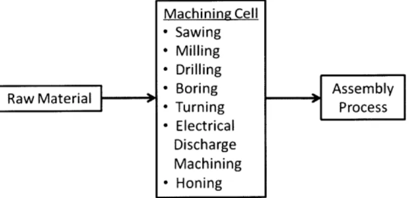
The general manufacturing process flow is shown in Figure 1-2 below. Machining Cell

- Sawing -Milling - Drilling

Raw Material - Boririg Assocey

- Electrical Discharge Machining - Honing

The manufacturing process begins with raw material coming in from Company X's suppliers. These raw materials go through various steps of machining in the machining cell before complete components are obtained. Completed components are then assembled together to make a complete product.

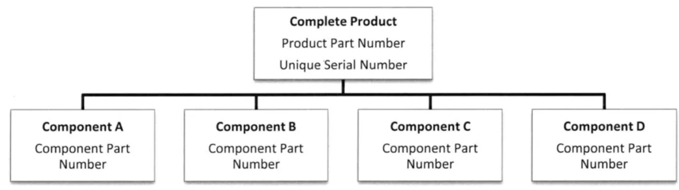
Company X's products are highly-customized in nature. As such, manufactured products are high in mix and low in volume. In order to keep track of manufactured products, product part numbers are used as identifiers. Each complete product, identified uniquely by its serial number and by its product part number for its type, is made up of various components, each identified by their component part numbers for their types. Figure 1-3 below illustrates this. The manufacturing process flow differs for different components in terms of machine routings through the machining cell depending on the specific type of complete product that is being manufactured. Currently, there are about 45 different complete product designs with about 125 different component designs. Each time a new product design with new features are released, new product part numbers are created.

Complete Product Product Part Number Unique'Serial Number

Component A Component B Component C Component D

Component Part Component Part Component Part Component Part

Number Number Number Number

1.3

Current Manufacturing Issues

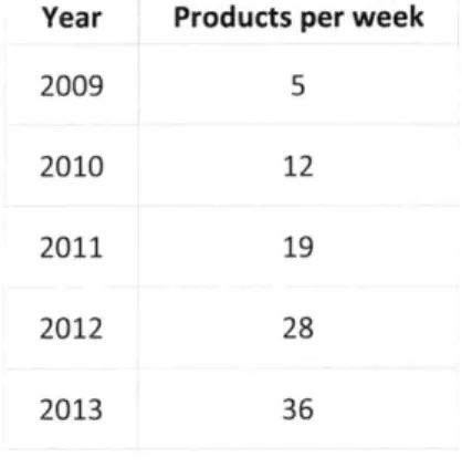
Significant growth in the product sales is expected in the coming years. In order for Company X to continue being the market leader, efforts to increase manufacturing capacity to meet customer demand with competitive lead time, cost, and quality has been put in place.

Table 1-1 below shows the projected number of products that need to be produced per week over the

next few years.

Table 1-1: Projected number of products to be produced per week

Year Products per week

2009 5

2010 12

2011 19

2012 28

2013 36

The current manufacturing capacity is able to produce a maximum of 10 products per week. Thus, to improve the throughput rate in order to meet the projected demand over the next few years, capacity expansion projects might become a need should the above trend in future demand materialize.

Also, current manufacturing lead times are much longer (ranging from three to five weeks) than total processing times due to excessive Work-In-Process (WIP). This results in high non-value-adding (waiting) times. It is noted that achieving less WIP will reduce waiting times and consequently reduce the manufacturing lead times. Shorter manufacturing lead times will in turn enable a quicker response to customer orders, ensuring better customer service and on-time delivery.

The abovementioned issues have various contributing factors. In particular, due to limitations in production planning and scheduling, unbalanced loading of machines in the machine cell causes less than the maximum machining capacity to be achieved as some machines are idling while others are overloaded. It also results in added disruptions when machinists are told to load an idle machine with a part that should originally be loaded to another overloaded machine by the Production Team Leader. These situations are unplanned for and unwanted as it limits the production capacity of the machining

cell. Engineers in the department are aware of this problem and have been trying to find a solution to it. This project seeks to address the limitations in production planning and scheduling that cause unbalanced loading and idling of machines as well as longer manufacturing lead times. Further discussion will follow in the coming chapters of this thesis.

1.4

Thesis Structure

This thesis is organized into seven chapters. Chapter 1 gives a brief introduction to the company, its manufacturing process, and key manufacturing issues that are currently faced. Chapter 2 gives a background on the problem, defines the problem addressed, and specifies the objective, goal, and scope of this project. Chapter 3 reviews relevant literature and highlights current practices in the industry. Chapter 4 details the methodology, work, and development that have been carried out throughout the thesis. Chapter 5 presents and discusses the obtained results and further evaluates the undertaken methodology. Chapter 6 gives recommendations for action to the company based on the results and analyses. Chapter 7 concludes this thesis' work and details other future work that has been identified. At the end of this thesis, relevant references are listed, as well as data appendices for the reader's reference, if desired.

Chapter 2:

Problem Statement

2.1

Thesis Focus

The focus of this thesis is to address the limitations in production planning and scheduling in the machining cell that potentially cause unbalanced loading and idling of machines as well as long manufacturing lead times. The following sections in this chapter will give a background on the problem and then detail the objective, goal, and scope of this project.

2.2

Background on Machining Process

As already mentioned, components of complete products are machined from raw material in multiple steps before they are assembled into complete sets of products. The specific machining processes are: Sawing, Milling, Drilling, Boring, Turning, Electro Discharge Machining (EDM), and Honing.

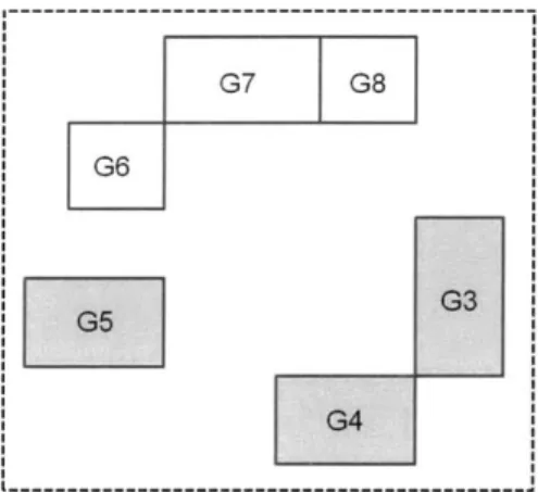
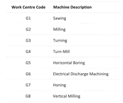
Figure 2-1 below shows the setup of the machining cell in the shop floor, and Table 2-1 lists the

machines that are in the production floor. It will be seen that G1 and G2 are not physically located within the machining cell. The Sawing, EDM, and Honing processes are each performed at their dedicated machines respectively: G1, G6, and G7. All other processes are performed at the three main machines (shaded blue in Figure 2-1) in the machining cell: the Turning machine (G3), the Turn-Mill machine (G4), and the Horizontal Boring machine (G5). Each component has to undergo multiple machining steps at these machines before they are passed downstream for assembly.

G7 G8

I G6

G3 G5

G4

Table 2-1: List of machines in the production floor

Work Centre Code Machine Description

G1 Sawing

G2 Milling

G3 Turning

G4 Turn-Mill

G5 Horizontal Boring

G6 Electrical Discharge Machining

G7 Honing

G8 Vertical Milling

Each unique component varies in size, material, and features, and thus would vary in its machine setup and machining steps. Consequently, the processing times for each of these machining steps would vary as well. There are also constraints on machine capabilities as to what component can be machined where. G3 is a turning machine with only one chuck that can be used for components of any length. G4 is a turn-mill machine with two chucks that has a length limitation on the components that can be loaded into it. G5 is a horizontal boring machine with a movable worktable that can perform any milling or turning step on any component length. Thus, there exists a job scheduling problem between the components and the main machines: which component should be allocated to which machine and in what order in order to achieve a balanced load on all machines, maximize the utilization (minimum machine idling time), and minimize the component waiting times (and thus manufacturing lead times and Work-In-Process).

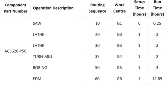
There currently are specific routes that each unique component would follow during its manufacturing process. Table 2-2 below shows an example of the machine routing for a typical component identified

by its part number from Operation 10 to Operation 60 in sequence. Again, different components will

Table 2-2: Routing sequence through the machining cell for a particular component

Component Routing Work Setup Run

Opeatin esciptonTime Time

Part Number Operation Description Sequence Centre

(hours) (hours) SAW 10 G1 0 0.25 LATHE 20 G3 1 2 LATHE 30 G3 1 2 AC5626-P50 TURN-MILL 35 G4 1 2 BORING 50 G5 1 3 EDM 60 G6 1 12.85

The workload for each week is released to the shop floor as a list of work orders at the start of the week, sorted according to earliest due date first. Each work order will specify only one component part number and the quantity to be manufactured. Work orders are typically sized with a batch size of 3 to 5 pieces. Machinists will begin to work on the work orders starting from the top of the list. Before each process step in a work order, there will be some time incurred in setting up the machine with the correct tooling, program, and material. The setups between identical components in a work order will naturally be quicker.

With this current practice, we found that for the three main machines in the machining cell (G3, G4, G5), certain machines will be overloaded while the others are idle due to- unbalanced loading across these machines. In response to this situation, the engineers in the department have decided to allow components to be loaded into an idle machine whenever this occurred (on an ad hoc basis) even though it should originally be loaded into another overloaded machine. However, this would involve creating the necessary CNC programming codes for machining that particular component and developing new setup procedures, since the idle machine has not originally been set up to machine that particular component. The first component that is produced then needs to go through an inspection as well before proceeding with the rest of the work order. This disruptive situation is unplanned for and unwanted as it limits the production capacity of the machining cell.

Currently, the machining cell is able to achieve an output of about 5 complete sets of product per week. Thus, we seek to develop a reliable method to be able to schedule components to be machined while

keeping loads balanced across the three main machines with high utilization in order to increase the overall machining output capacity.

2.3

Project Objective, Goal, and Scope

Based on the above, this project will have the following objective:

e To develop an improved method to schedule production of product components across the machining cell without potentially causing unbalanced loading and idling of machines as well as long manufacturing lead times

This will lead to the goal of having:

* An increase in the overall machining cell output capacity and a reduction in overall manufacturing lead times and WIP levels due to higher machine utilizations and better production planning.

The above objective will be within the scope of:

Chapter 3:

Literature Review

3.1

Introduction

This chapter will review two key areas in the development of this thesis' work. Job shop scheduling will be reviewed to understand how it is applicable to the problem in this thesis, and the use of production planning and scheduling tools in the industry today will be briefly highlighted.

3.2

Job Shop Scheduling

The machining cell encountered is equivalent to a job shop production, since it uses shared machines and is highly flexible without a fixed flow for all parts. Parts are high-mix and low-volume in nature and are produced in small batches. It is not necessary for all machining steps to be performed on all parts, and their sequence may be different for different parts as well [1].

Scheduling involves the allocation of scare resources to activities with the objective of optimizing one or more performance measures, subject to certain specific constraints. In this case, the resource would be the machines in the machining cell, and the activities would be the various operations for the manufacturing of the product components. The performance measures to be optimized would be the utilization of machines, manufacturing lead time, makespan, work-in-process (WIP) levels, and throughput. Constraints would be the time taken to setup and run a particular part, which operations need to be completed for a particular part, which machines are able to complete which particular operations, and any precedence requirements for the execution of a particular operation.

The study of scheduling is also applied in many fields other than manufacturing such as computer systems, airport runway systems, and the like. In manufacturing, job shop scheduling is a well-known problem and has presented itself in many forms. A vast number of techniques have been proposed as solutions to different job shop scheduling problems and range from executing dispatching rules for simpler problems to using heuristic search algorithms for solving more complex simulation models. Scheduling methods can also be either static or dynamic. As for dispatching rules, Shortest Processing

Time first (SPT) performs well in minimizing average flow time (manufacturing lead time) and makespan as well. Earliest Due Date first (EDD) minimizes maximum lateness or tardiness. [2]

In production scheduling, an active schedule is one that never makes a job wait in queue when it can be completely processed before the next job is scheduled to start. Active scheduling reasons that by going ahead and producing the job, nothing is delayed and time that would otherwise be wasted is used productively. Nondelay schedules are such that a machine is never idle when there are parts waiting in its queue. In nondelay scheduling, a job is started if it can be started before the next job is scheduled to start. For regular measures of performance that are nondecreasing in job completion times, such as makespan, flow time, lateness, and tardiness, the optimal schedule would be an active schedule. A nondelay schedule may not be optimal but will typically be close. Nondelay schedules also tend to achieve high resource utilizations by following the oft-imposed organizational expectation that machines do not sit idle while there is work in their input queue [2].

3.3

Production Planning and Scheduling Tools

Manufacturing systems simultaneously need to meet due dates, deal with an amount of work in process inventory, and minimize the possibility of low resource utilization. This is made complicated even further in make-to-order companies that manufacture high variety of products in relatively low volumes, as they typically do not hold finished goods inventory, being very difficult to predict customer requirements. In this environment, complex product structures have many part types and each has a small quantity order size. Consequently, the lead time required to complete all the jobs is high with uncertain product routings and processing times. Such uncertainty, coupled with uncertainty in customer orders, makes production planning and control very difficult to manage. Thus, there has been a need for better production planning tools in the manufacturing industry to cope with the competitive demands of customers [3].

Many commercial project management and scheduling programs have been available in the market, such as Microsoft Project, Primevera Project Planner, Project Manager Workbench, Project Scheduler, and more. Gradisar and Music proposed scheduling production activities using these project planning tools [4]. A comparison between project management and production planning and scheduling techniques was presented and a uniform approach was developed to enable use of project planning

techniques in the area of production systems. They then proceeded to apply it to a model of a multi product batch plant using the industry-accepted project-planning tool Microsoft Project. Their solution of job scheduling was proposed to be further included in an Enterprise Resource Planning (ERP) system with which orders were generated.

Kolisch performed a study on the quality of seven different commercial project management software packages in allocating resources, and noted how project management has become a widely and successfully used methodology for planning, steering, and controlling single and complex undertakings, such as production planning and control [5].

Crawford, in his proposal for a new approach towards resource constrained project scheduling (RCPS), noted how RCPS is a generalization of job shop scheduling and is a good model for problems that even

job shop problems cannot express. He further noted how Microsoft Project, arguably the most widely

used commercial scheduling program, seemed to capture exactly the same optimization problem as RCPS with its resource leveling function [6], and thus would be a suitable tool for job shop scheduling. Roberts performed a thesis research in developing a Visual Basic scheduling tool that will aid in the creation of repetitive job schedules in Microsoft Project for a lean manufacturing environment [7]. His development significantly reduced any manual work on Microsoft Project and when combined with Microsoft Project's scheduling abilities, produced a quick and robust scheduling tool for the production activities at the Naval Surface Warfare Center in Crane, Indiana.

In the industry, Capstone Planning and Control Inc. developed a pre-production process management system based on Microsoft Project 2002 and marketed it as a holistic web-based approach to

pre-production process management, having traced various issues faced by the manufacturing industry to arise from poor pre-production planning [8]. Microsoft Project 2002 was chosen due to its ease of use, the cost relative to other products, its integration with other Microsoft products, ease of customization and deployment, and the ability to incorporate their clients' manufacturing processes into the product. Jobscope was another company that was established to develop manufacturing and ERP software to

meet the requirements of job-based manufacturing (e.g. make-to-order) that were not being met by traditional manufacturing software solutions [9]. They too developed a system that interfaced with

3.4

Summary

With the above literature review, we developed a methodology to achieve the project objective as defined in Section 2.3 earlier; we describe this methodology in the next chapter.

Chapter 4:

Methodology

4.1

Introduction

Based on the literature review, and also because the company already owned a copy of the software, we decided to proceed with using Microsoft Project 2007 as a tool for developing the improved method for production planning. However, before it could be used effectively, relevant data had to be obtained beforehand. This chapter outlines the work that has been performed according to the Six Sigma Quality Improvement Methodology as a guide. The project roadmap of Define, Measure, Analyze, Improve, and Control were carried out in the following five phases.

4.2

Defining the Problem and Understanding Its Background

The current scheduling practice and flow of parts in the production floor were observed in order to understand the problem at hand. Observations were made by being in the production floor and watching the machinists while they work. Input and feedback were also obtained by communicating with the machinists and engineering team (Machining Engineering Team Leader, Machining Engineer, Production Team Leader, Production Planner) in the engineering department. Frequent interviews and discussions with them helped in understanding and clarifying the current scheduling process and its limitations further and also highlighting key issues.

4.3

Measuring and Collecting Relevant Data

4.3.1 Process Run Time Data

Static system data for process run times and setup times for all components were available from the MFG/PRO system. The MFG/PRO system is an integrated enterprise resource planning (ERP) system that was used in the Sales and Distribution, Manufacturing, and Financial departments in the manufacturing facility. The manufacturing functionality of the system included management of Work Orders, Shop Floor Control, Routings, as well as Product Structure. However, the static setup and run times contained

in the MFG/PRO system were outdated and greatly underestimated as they were only applicable to operations in a previous facility before they were transferred to the current facility. Therefore, actual data had to be obtained directly from the shop floor. In practice, machinists manually fill up log sheets and also clock in and out of the MFG/PRO system each time they start and complete a setup procedure or a run procedure. Thus, raw data from this source were extracted as text files and imported into Microsoft Excel spreadsheets. The average times over many repeated operations were calculated and used to represent the actual timings of those operations. These calculated average times were then compared to the manual log sheets to check for data consistency. Only run time data from January to June 2010 was collected to ensure that the data were up to date. The following subsections detail the above.

4.3.1.1 Data Extraction from MFG/PRO System

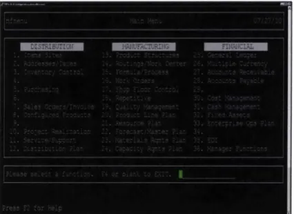
The MFG/PRO system was accessed via the company-wide network. The user interface can be seen in the screenshot below in Figure 4-1. The keyboard was used to maneuver within the program.

Figure 4-1: Screenshot of the main menu in MFG/PRO

The three main functions in MFG/PRO can be seen, namely Distribution, Manufacturing, and

Financial. Only the Manufacturing function was used in this project. The Manufacturing function .... .... ... .-, " - --- I

---encompasses various sub-functions, and all run time data were obtained from item 17. Shop

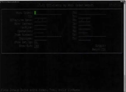
Floor Control as seen above. The following screen in Figure 4-2 is seen when selecting 20. Efficiency by Work Order Report in the subsequent menu.

Figure 4-2: Efficiency by Work Order Report screen

In the Efficiency by Work Order Report menu, desired details can be entered into the query fields and the system will then output the queried data accordingly. For example, by entering an

Effective Date range and a Work Center code, all components machined on that particular

machine within the specified range of dates will be output, together with their operator, quantity, and run times. By further specifying a particular Item Number (component part number) and Operation number, only those operations performed on components machined within the specified range of dates on that specific machine will be output. In this manner, the

user can easily extract any production history data just by specifying what is wanted.

In order to obtain run time data for all machined components in the period January to June 2010, the Effective Date range was specified. This was performed repeatedly for each Work

Center at a time in order to limit the amount of data that was extracted at a time so that it was

manageable. Thus, all Work Orders completed within the specified Effective Date range with all

Operations performed on all Item Numbers by all Employees were extracted, one Work Center at

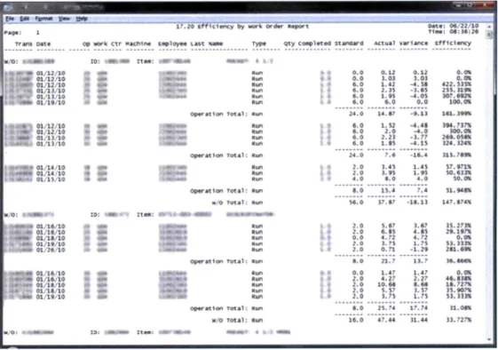
a time. The option to output it as a text file was selected. Figure 4-3 below shows an example of the data output from MFG/PRO.

op wcrk ctr Wackine * -* a .4* Pa:e 1 Trans ate 4k 04 0: I Ien o - 01,12 10 - e 01112 o0 01. 1,10 031 110 I 01 11 10 60 01 19 11) 01 0L12,10 01-12 10 aMW 01. 13 to at 01 10 o --af 01"14 1* M0: a, Is 4 an 01 16-to diAh4 01 16'10 -'44" 021 10,to anat :6 Lo C -W 4 01 1i '10 9 1 10 10 at+ -1Is 10 oft W1-19 10 Item:

17, 20 6fficietCy by or6 oroer epow

Lgplaye tast %m Tye q[Y Caimpleted Stard0r Actual WaI&nKe

un. 0.12 0..2 Mun 0.0 1.03 LO3 ,Run Oe,0 42 -4.$# - - tu 4 , 0 2,37 -3.95 Nun,0 19 -4.0$ Run 4.0 0.0

pration Tota; Sun 24.0 14.7 9.13

RMk, 4#An.0 1 A4#44 Run 6.0 2.0 -4.0 Run 6 9.0 2.21 -1.77 -un 6.0 LAS ~4.15 eger at Tota : 24.0 7.6 -16.4 iR1 2.0 1.41 1.4% amu 7.0 ) .9$ 1$ nn 4,0 6.0 4,0 peration Tota- s, 5.0 114 7,4 wo local; Nun 5.0 37.67 -14.13 awn 2.0 1.67 L K Lift2.0 6.61 4.61 -um 0.0 4.72 4.72 Run 1.0 l7 1.71 ---- .0--L - 0.7 -19-qpratten Totah- , 6,0 271, 11,7 - -- Sun 1.,L47 1.47 o 2.a L0 4.27 27 ? Run 2.0 10.4 .44 Own 2.0 S.57 1,17 un2.0 1.7 1.7 Certion Totah l.n '.0 2.74 17.74 .0 TOW: RI 16.0 47.44 31.44 -* *40,0 , .me , m fi.; 04:2/10 0. O l25. J01 107, O92 300.06 16.63966 )U.27% 300.06 324.324% U7- 71 0.065 $1. 9436 147. 3746 31 2716 29.1976 0.06 24L.4w 36.0466 0.06 465316 16.7276 $3. 3336 12.7276

Figure 4-3: Data output from MFG/PRO as a text file

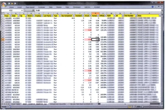
4.3.1.2 Data Manipulation in Microsoft Excel

In Figure 4-3, we see that columns of data were already in place in the text file, making it easy to import into Microsoft Excel as fixed-width data. However, the data were also separated into sections according to each Work Order ID with horizontal separators and thus some manual rearranging had to be done after importing into Microsoft Excel. Figure 4-4 below shows an example of the data in Microsoft Excel in a table after rearranging has been completed. Each column represents a type of information, while each row is an entry of information. Filters and conditional formatting were used to help browsing through the extensive data, and the data was sorted according to Part Number, Operation, and Date for easy viewing.

pm pm

-o. 4*

4-w.

:::: - - '. -- "' " - 11-1111-111, "I'll I I'll, "1 11 11 - - - - - - - __ --- - - - - - - - - - I ___ - R . ... .. ... __ _

Figure 4-4: Data arranged in Microsoft Excel

In order to obtain average actual run times, all entries of a particular operation on a particular component part number on a particular machine were considered. From all 3,000 entries of run time data, a pivot table was used to sum the total actual times and then divide that by the total quantity completed for each operation on a particular component part number on a particular machine. This gave the average actual run times for all operations on all components over the period January to June 2010, and can be found in Appendix A.

4.3.1.3 Comparing with Production Log Sheet Data

The average run times were then compared to production log sheets that are filled in by machinists manually by hand in order to check for consistency. Numbers from both sources agreed well with each other with no alarming differences; some examples are shown in Table

4-1 below. Variations can be due to allowance for manual handling of parts. Some components

had a low number of observations as they were low in demand.

...

Table 4-1: Comparison of calculated average run times and Component Part Number AA0898-T72 AA0898-T74 AC5626-P50 AC5626-P51 AC5626-P52 AE7768-P89 AE7772-P70 AE7915-P20 S05326-Y35 SO5760-Y21 Operation Number 30 30 50 76 40 20 30 40 20 40 Calculated Average (hours) 1.17 1.63 12.54 5.69 1.85 1.59 1.25 2.98 0.71 1.49

timings from production log sheets

Number of

Observations Sample from

forvalcats Production Log

for Calculated She(ous Average Sheet (hours) Average 2 1.75 1.33 13.00 5.17 1.83 1.50 1.25 3.33 1.00 1.50

4.3.2 Other Relevant Data

Besides setup and run times data, current machining output capacity was 5 complete sets of product per week with a manufacturing lead time of about 3 weeks in general. Historical sales data for completed components in the period December 2008 till June 2010 were also obtained from Sales personnel and this data were used to identify those components that are high runners in order to be able to focus on them and not the vast number of components. Components with a total quantity sold of greater than 30 pieces were shortlisted, and a total of 16 out of 125 components (12.8%) were identified as contributing to 45.6% of total sales volume and are shown in Table 4-2 below. The complete list of components that were sold between December 2008 and June 2010 can be found in Appendix B.

Table 4-2: List of high runner components

according to sales data from December 2008 till June 2010 Component Part Number Quantity Sold

S05326-Y35 74 S05568-Y25 64 S05428-Y25 60 S05568-Y35 60 AC5626-P50 43 AC6114-P25 38 S05568-Y45 37 AC5626-P52 36 S05724-Y62 35 S05568-Y15 34 S05568-Y55 34 S05760-Y34 33 AC5626-P51 32 AC6099-P12 31 AC6099-P49 31 AC6113-P58 31

4.4

Analyzing Collected Data and the Current Scheduling Process

From the list in Table 4-2 above, the average actual timings for these high runners were compared to their system timings to check for any large discrepancies. Those operations with large discrepancies were highlighted so that their timings could be manually updated when entering them into the production schedule. However, only averages that were calculated over a completed quantity of greater than 5 (refer Appendix A) were taken into consideration to ensure reliability of the data. This will be further described in Section 4.5.2 later.

4.4.2 Analysis of Current Scheduling Process

Having obtained all of the above data, we proceeded to evaluate the current scheduling process, leading us to find certain limitations and drawbacks. These included blind spots which impeded the effectiveness of the actual production schedule. In particular, scheduling was performed using the outdated MFG/PRO system timings and this reduced the accuracy of the schedules. A rough rule of thumb of adding 50% of run times to all components was used to account for the underestimated timings. Also, scheduling for a week was planned in terms of the total required work hours only; as long as the total required work hours for the week did not exceed the available hours for each machine, the schedule would be released to the production floor in order of earliest due date first. However, the requirement for a predecessor operation to be completed before a particular operation can begin was not captured at all, as the total required work hours was merely a sum of work hours required for all components assigned to be machined at a particular machine. Should a predecessor operation of a particular operation not be completed yet, that particular operation cannot actually begin and should not be included in the schedule at all or included in the total required work hours for that week. It was also frequently found that the required work hours for the three main machines (G3, G4, G5) in the machining cell were not balanced with one or two overloaded while the others are idling. In order to utilize the idle machines as much as possible, operations for work orders further down the list will sometimes be brought forward and performed first.

In analyzing all of the above observations, it was clear that a major problem was that there was insufficient visibility on how the tasks were being carried out at the production floor at the machines and when exactly machines will be idling. Predecessors of operations were not taken into consideration for planning as well. This limited advanced detailed planning and led to the fire-fighting nature of planning as described above.

4.5

Improving Current Practices

4.5.1 Using Microsoft Project 2007 as a Modeling Tool

As an improved method for scheduling and planning in the machining cell, Microsoft Project 2007 was used. Several resources were used to aid in the development process [10], [11]. A Gantt chart of the production plan for the entire list of work orders could be produced and weekly details could be observed when zooming in the timeline. The list of work orders, their durations, and deadlines could be extracted from the MFG/PRO system into a Microsoft Excel spreadsheet and then imported into

Microsoft Project 2007 directly, making setting up the Project file straight forward. Tasks were listed according to earliest deadline first. Machines were defined as Resources and their available working hours were defined. Each work order was entered as a Task that was assigned to a Resource for a specific Duration. Predecessors were also defined for operations that required them. Microsoft Project

2007 would then lay out a Gantt chart for each Task that is listed according to their Resource

assignments. Any Task that had a completion date that exceeded the stipulated deadline would be highlighted, indicating that the schedule would need adjustments.

By using Microsoft Project 2007, a visual representation in the form of a Gantt chart would be available

for the Production Planner and machinists to visualize which machines should be running on which components and exactly when. All Tasks can also be easily checked to see that they are completed before their deadlines. Having predecessor operations defined also helps to ensure that the production planning is realistic and feasible as Microsoft Project would not schedule any Task to be run before its predecessor operations were completed. Tasks could also be manually assigned priorities in case specific tasks had to be expedited. The Resource Usage view allows the user to check the utilization of the machines on a daily basis to see if they are over-allocated or balanced. The following subsections further describe the above with screenshots of setting up Microsoft Project 2007 with a list of work orders; the same list of work orders has been used throughout as an example.

4.5.1.1 Importing Task Data

Released work order data could be extracted from the MFG/PRO system directly into a Microsoft Excel spreadsheet. From there, task data was easily imported into Microsoft Project

by matching the respective fields in Microsoft Project to the corresponding column labels in the

Microsoft Project directly and can be seen in Figure 4-5 below. Prior to importing, the work order data were sorted according to due date, work order ID, and operation in Microsoft Excel.

Figure 4-5: Import Wizard in Microsoft Project 2007

4.5.1.2 Gantt Table, Predecessors, and Priorities

Imported data would appear in Microsoft Project in the Gantt Table, as seen in Figure 4-6. Other

relevant data were then entered accordingly, such as Predecessors, Constraint Type and Date, and Priorities. The Constraint Type was set to Finish No Later Than, and the Constraint Date set to be same as the Deadline.

Predecessors were defined by using ID numbers (leftmost column), e.g. if a particular task has the number 2 in its predecessor column, it means task 2 is a predecessor to that particular task.

In the example below, task 3 has task 2 as its predecessor.

Assignable priority values range from 0 to 1000, with 500 being the default priority for all tasks. Priority values are arbitrarily assigned, with a smaller priority value indicating a lower priority. A task assigned with a priority of 1000 means that Microsoft Project should not reschedule that task or change its start date, while 999 is the highest priority assignable to a task while still

allowing it to be rescheduled. Higher priority tasks are always scheduled before lower priority tasks, and lower priority tasks are not allowed to delay higher priority tasks.

Part Nunter Predec Operahln Duraton Machie AE8071-P58 60 221 hrs GS AE8071-P62 35 13 hrs G5 AE8071362 2 40 6.5 hrs G7 AE8071-P62 3 50 6.5 hrs G5 AE8071-P62 4 55 11.7 hrsi G4 AE8071-P62 5 60 9.62 hrs G7 AE8072-P20 20 13.65 hrs G4 AE8072-P24 20 6.5 hrs G5 AE8072-P24 8 30 7.54 hrs G3 AE8072-P24 9 40 5.77 hrs G3 AE7864-P96 35 3.9 hrs G4 AE7864-P96 11 50 5.2 his G5 AE7864-P96 12 60 68.12 hrs G6 AE7864-P98 40 13.57 hrs G4 AE7864-P98 14 50 16.9 hrs G3 AE7864-P98 15 60 6.5 hrs G4 AE7864-P98 16 70 16.9 hrs GS AE7864-P96 20 9.1 hrs G3 AE7864-P96 18 30 9.1 hrs G3 AE7864-P96 19 35 9.1 hrs G4 AE7864-P96 20 50 13 hrs G5 AE7864-P96 21 60 51.42 his 06 AE7864-P96 40 10-5 hrs G4 AE7864-P96 23 50 13 hrs G3 AE7864-P96 24 60 52 hrs G4 AE7864-P96 25 70 13 his G5 AE8072-P30 20 7 15 hrs G4 AE8072-P30 27 30 7.15 hrs G4 AE8072-P30 28 50 8.45 hrs jG8 D-0-n I Priarty I Sht Sat 24/710 800 Mon /7/10: 1 556745 2 556778 3 556778 4 556778 5 556778 6 M 556778 7 556779 8 557867 9 5577 10 557867 11 557870 12 557870 13 557870 14 557911 15 557911 16 557911 17 557911 18 558013 19 558013 20 558013 21 556013 22 558013 23 558055 24 558055 25 558055 26 558055 27 558164 28 558164 29 558164 Mon 517/10 Mon 5/7/10 Man 5/7/10 Tue 6/7/10 Tue 6/7/10 Mon 517110 Mon 517/10 Mon 5/7/10 Mon 517/10 Mon 5/7/10 Mon 517/10 Mon 5/7/10 Mon 5/7/10 Mon 517/10 Tue 6/7/10 Tue 6/7/10 Mon 517/10 Mon 517/10 Mon 5/7/10 Tue 6/7110 Wed 717/10 Mon 5/7/10 Mon 5/7110 Tue 6/7110 Tue 6(7/10 Mon 517110 Mon 5/7/10 Mon 5/7/10

Ftht Co aintType Consbaint Date Tue 6/7/10 Fntsh No Later Than Sat 2417110 Mon 517110 Finish No Later Than Sat 24/7/10 Mon 5/7/10 Fnsh No Later Than Sat 24/7/10

Tue 6/7/10 Fis/h No Later Than Sat 24/7/10 Te 617/10 ish No LaterThani Sat 24/7/10 Wed 5/7/10 Fins/h No Later Than Sat 2417/10 Mon 51710 Fntsth No Later Than Sat 2417/10 Mon 517110 Fis/h No Later Than Sat 2417/10 Mon 5/7/10 Finsh No Later Than Sat 2417/10 Mon 517/10 Finish No Later Than, Sat 2417110

Mon 517/10 Fhi Na Later Than Wed 28/7/10 Mon 8/710 Finish No Later Than Wed 28/7/10 Thu 8M7/101 Fntsth No Later Than Wed 28/7/10 Mon 5/7/10 Fitnsh No Later Than Wed 2817/10 Tue 67/10 FWh NO Later Than Wed 28/7/10 Tue 71/10 Fins No Later Than Wed 28/7/10 Wed 7/7/10 Fnsh No Later Than Wed 2817/10 Mon 5/7/10 Finish No Later Than Wed 28/7/10 Mon 517110 Fnsh No Later Than Wed 28/7/10 Tue 6f//10 F/s/h No Later Than Wed 28/7/10 Wed 717/10 Fnitsh No Later Than Wed 28/7110

Fn 917/10 Finish No Later Than Wed 28/7/10 Mon 5/710 Fets/h No Later Than Tue 3/8/10 Tue 6/710 Finsh No Later Than Tue 3/8/10 Tue 617110 Fettsh No Later Than Tue 3/8/10 Wed 717/10 Fish No Later Than Tue 318/10 Mon 517110 Fesh No Later Than Tue 3/8/10 Mon 5/7/10 F/ish No Later Than Tue 3/8/10 Tue 6/7/10 Fih No Later Than Tue 3/8/10

Figure 4-6: Gantt Table in Microsoft Project 2007

In the Gantt Table, each row represents a task, and each task represents a batch of components to be machined. In the production floor, setup durations between runs within a single batch were not recorded separately, but were always recorded as a part of the run times. No separate data was available for setup durations between runs within a single batch, although data for setup durations between batches were available. Thus, the duration specified for each task in

Microsoft Project is the sum of the time taken to perform the first setup between batches with the total run time to complete the entire batch, i.e. ((first setup) + ((batch size)x(run time)));

each batch is assumed to be setup only once.

Multiple rows with the same work order ID (WOID) are operations that belong to the same work order to produce a batch of a particular component part number. For example, tasks 2, 3, 4, 5, and 6 are operations that belong to the same work order in order to produce a batch of components with part number AE8071-P62.

Sat 2417/10 Sat 2417/10 Sat 2417/10 Sat 2417110 Sat 2417/10 Sat 2417/10 Sat 24/7110 Sat 2417/10 Sat 2417110 Wed 2817/10 Wed 28/7110 Wed 28/10 Wed 2817/10 Wed 28/7/10 Wed 2817/10 Wed 28/7/10 Wed 28/7/10 Wed 28/7110: Wed 28/7/10 Wed 28/710 Wed 28/7/10: Tue 3/8/10 Tue 3/8/10 Tue 3/8/10 Tue 3/8/10 Tue 3/8/10 Tue 3/8/10 Tue 3/8/10

4.5.1.3 Gantt Chart

Task data in the Gantt Table would be reflected in the Gantt Chart as well. Their predecessors, durations, start and end dates, and allocated resources could be clearly seen. However, loads at this point were not yet leveled across the resources and many allocation clashes could be seen since all tasks were starting at the same time, as Microsoft Project would schedule all tasks to start on the defined project start date as soon as possible by default. Capacity constraints of the machines are ignored at this stage.

Figure 4-7 below shows an example of the Gantt Chart showing a few work orders from the list

in Figure 4-6. Tasks 2, 3, 4, 5, and 6 make up one work order, as they have the same work order

ID in Figure 4-6. It can be seen that for this work order, an operation had to be completed on G5

before the next operation on G7 was started. This is due to the predecessor finish-start dependency defined between tasks 2 and 3. This results in the chain of tasks from G5 to G7 to

G5 to G4 to G7 for tasks 2 to 6 respectively. Arrows on the right side of the chart indicate the

defined deadlines.

5 JuliO 2 JuI10 19 Jul 10 26Ju'10 2Au *1 97 Aug S S M T|W|TIFIS S M T WITIF|S S MIT W T F S|S MIT W|T F S S MIT W|T F S SIM T

7 G4 3 G7 12 G5 G6 18 G4 27 G4 G4 19 20 T.G 22 G6 23

~G4

~G4

Figure 4-7: Gantt Chart 33

4.5.1.4 Resource Sheet

In the Resource Sheet, the various machine names could be seen. Any machine that was highlighted red indicated that the machine was over-allocated. In Figure 4-8 below, machines are highlighted red due to over-allocated resources with allocation clashes as seen in Figure 4-7 above, e.g. tasks 13 and 22 are allocated to machine G6 at the same time. The Base Calendar for each machine was set to define the normal daily working hours for each machine in a working week. The availability of machines (Available From, Available To) could also be set to easily account for machine downtime.

0 Mac~ie Type Max. unts Availabe Avalabe I Casecndar To From

1 $t G5 Work 100% NA NA 20 Hours 2 $ G7 Work 100% NA NA 20 Hours 3 J) G4 Work 100% NA NA 20 Hours 4 G1 Work 100% NA A20 Hours 5 $ G3 Work 100% NA NA 20 Hours 6 4) G6 Work 100% NA NA 20 Hours

- G8 Work 100% NA A 20 Hours

Figure 4-8: Resource Sheet in Microsoft Project 2007 4.5.1.5 Resource Usage

The Resource Usage view, as in Figure 4-9, showed the daily usage of each machine with the current infinite-capacity production schedule. Again, days with over-allocated resources were highlighted in red. From here, it could be seen if loads across the 3 main machines, G5, G4, and

G3, were balanced or not. We see that all required work hours were crammed into a few days

(as soon as possible) initially before any resource leveling was implemented, corresponding to all tasks starting at the same time. Resource leveling would later be used to allocate tasks according to the available daily capacity of each machine.

5 Mea T W T F S S M2J T 1 MA hrs Work 6795 61.85h 6397h 7665 26.12 2 $ +G7 SO hrs 23h 4482 12 3 4) + G4 476M hrz Work 2152 1414h 70326 M867 11326 4

K~~

8

Figure 4-9: Resource Usage in Microsoft Project 2007 ... .... .

4.5.2 Fine-tuning the Scheduling Model

Further fine-tuning was performed on the schedules developed in Microsoft Project to obtain a more realistic model of the actual production floor. In order to define the available daily capacity of the machines, the number of available hours per day was reduced from 24 hours to only 20 hours and the number of working days per week was reduced to six, with Sunday set as a non-working day. Figure 4-10 below shows the Change Working Time window in Microsoft Project where the daily working hours in a working week was defined.

Forlndr: 20 Hours (PoectCnd) t t C

Cdendar20 Hun is a base calendar.

Legend: Cd an a day to we iardng iMes:

14ki T W Th F SS

61td 5 6 7 8 9 10 11 12 13 14 15 16 17 i

On ftcalader:- Baed arc

19 20 21 122 2 Z3 24 25

26 27 29 30 31

-xmb Wnk Weed.

Figure 4-10:

To account for underestimated system timings, task durations were generally entered as 33% longer (value obtained by averaging all timing differences of less than 1 hour between actual and system timings). However, for those identified high runners with large discrepancies (greater than 1 hour) in timings, the calculated average actual timings from Appendix A were manually entered into the production schedule instead. Tasks that had timing differences greater than 1 hour but were low runners were not taken into consideration in our current analysis due to their low occurrence. Sawing operations (Operation Number 10) were also ignored due to its much shorter run times, making it an insignificant process in the total machining time. The list of high runners with run time discrepancies of greater than 1 hour are shown and discussed in Table 5-1 in the next chapter.

4.5.3 Resource Leveling

A feature of Microsoft Project 2007 that was particularly useful was the Resource Leveling feature. By

executing it, the workload on all Resources (in this case, machines) would be leveled out. This would avoid over-allocations and smooth out the workload by delaying tasks that had later deadlines. As resource allocation methods employed in commercial project management software packages are proprietary information, the algorithm or rules by which this is performed is not known exactly [5].

However, the Resource Leveling feature can be set in three ways in the Resource Leveling menu:

" ID only: Tasks are leveled based on their ID numbers with higher priority given to the tasks

higher up in the Gantt Table (smaller ID number, starting at 1) before considering the tasks that followed below (larger ID number), i.e. tasks higher up in the Gantt Table with smaller ID numbers had higher priorities. By observation, the tasks above are scheduled as soon as possible from the project start date by default, before the tasks below are squeezed in anywhere time is available on the required machine. This is effectively an active schedule as it will only schedule a task to be run if it can be completely processed before the next task in line is scheduled to start on the same machine.

* Standard: Tasks are scheduled as soon as possible by default, but examined for predecessor dependencies, slack, dates, assigned priorities, and constraints to decide which tasks should be delayed. By observation, tasks are started if it can be started before the next task is scheduled to start on the same machine. Thus, it is effectively a nondelay schedule. If more than one task is ready for the machine, the one with the earlier due date and/or longer remaining work is scheduled first.

* Priority, Standard: Assigned task priorities are checked first before the other standard criteria

are considered. Thus, a nondelay schedule is still produced, but with priorities given to specific

4

tasks to be scheduled before others as defined by the user. This gives the user further flexibility to influence how Microsoft Project schedules tasks.

Resource Leveling in Microsoft Project was set to look for over-allocations on a minute-by-minute basis as seen in Figure 4-11, since task durations were entered in fractions of hours. Microsoft Project was not allowed to split up single tasks (operations) in any way as this would not be practical in the actual production floor.

Levern dgatnon

© estmatic @Hnu

took for gverdoaocns on a MKinute by Mnute basis wOearievefnvalesbeforeleeig

Leveing range for 'PLYLM ad**igoea&g_07MIa10_C2

(0 Leveleire project

0 Levd Eu: Mon 5/7/10

t0: Thu 29/7/ 10

Resoivingoverilocaon

Leveg order:

[-Level ony it availablegdak

FILeveing can a~id Vidual assignments on aS~roiysadr

1Leverg neate spit in emm*V work1 "

tFILevel resourceswith the gpoased booIng type

Figure 4-11: Resource Leveling menu in Microsoft Project 2007

In order to level resources, Microsoft Project delayed tasks so that only one task was scheduled at any resource at any time, preventing any clashes. The Gantt Chart in Figure 4-12 below shows an example of the allocated tasks when leveled across resources using the Priority, Standard setting. Compared to the Gantt Chart in Figure 4-7 earlier, tasks on the same machine no longer start at the same time as some were delayed to make way for other tasks.