To cite this version :
Moghaddam, Alireza Attari and Kharaghani, Abdolreza and Tsotsas,
Evangelos and Prat, Marc
Kinematics in a slowly drying porous medium:
Reconciliation of pore network simulations and continuum modeling.
(2017) Physics of Fluids, vol. 29 (n° 2). pp. 1 -13. ISSN 1070-6631
O
pen
A
rchive
T
OULOUSE
A
rchive
O
uverte (
OATAO
)
OATAO is an open access repository that collects the work of some Toulouse researchers
and makes it freely available over the web where possible.
This is an author’s version published in :
http://oatao.univ-toulouse.fr/19955
Official URL :
https://dx.doi.org/10.1063/1.4975985
Any correspondence concerning this service should be sent to the repository administrator :
Kinematics in a slowly drying porous medium: Reconciliation
of pore network simulations and continuum modeling
Alireza Attari Moghaddam,1Abdolreza Kharaghani,1,a)Evangelos Tsotsas,1 and Marc Prat2,a)
1Otto-von-Guericke University Magdeburg, Universitaetsplatz 2, 39106 Magdeburg, Germany 2INPT, UPS, IMFT (Institut de M´ecanique des Fluides de Toulouse), Universite´ de Toulouse,
6 All´ee Emile Monso, 31400 Toulouse, France and CNRS, IMFT, All´ee du Professeur Camille Soula, 31400 Toulouse, France
We study the velocity field in the liquid phase during the drying of a porous medium in the capillarity-dominated regime with evaporation from the top surface. A simple mass balance in the continuum framework leads to a linear variation of the filtration velocity across the sample. By contrast, the instan-taneous slice-averaged velocity field determined from pore network simulations leads to step velocity profiles. The vertical velocity profile is almost constant near the evaporative top surface and zero close to the bottom of the sample. The relative extent of the two regions with constant velocity is dictated by the position of the most unstable meniscus. It is shown that the continuum and pore network results can be reconciled by averaging the velocity field obtained from the pore network simulations over time. This opens up interesting prospects regarding the transport of dissolved species during drying. Also, the study reveals the existence of an edge effect, which is not taken into account in the classical continuum models of drying.
[https://dx.doi.org/10.1063/1.4975985]
I. INTRODUCTION
Evaporation from a porous medium has been a subject of interest for decades in various fields such as soil physics,1
drying of manufactured products,2or remediation of soils
con-taminated by light hydrocarbons,3to name only a few. It is still
a very active field of research not only because of the contin-uous emergence of new applications, such as evaporation in fuel cells4or in loop heat pipes,5for example, but also because evaporation in porous media is not yet completely understood. Many aspects are still to be described, e.g., Refs.6and7. As in many previous works, we consider capillary porous media in this paper, i.e., porous media for which the pore size is typ-ically in the micrometer range (up to, say, sizes in the order of 100 µm). As described in many works, e.g., Refs.8and9, the drying kinetics of a capillary porous medium sample under typical room conditions (i.e., temperature close to 20◦C) can
be divided into three main stages: a first stage, the constant rate period (CRP), in which the evaporation rate is constant, a second stage called the falling rate period (FRP) in which the evaporation rate rapidly decreases, and a last stage, the receding front period (RFP) characterized by a receding inter-nal evaporation region. In both the CRP and FRP, liquid is present at the surface whereas the surface is dry during the RFP.
Another element of significance for the physics of drying is the liquid distribution during the process. This distribution is generally characterized using the concept of saturation, i.e., the fraction of the pore space volume occupied by a liquid.
a)Authors to whom correspondence should be addressed. Electronic
addresses: [email protected] and [email protected]
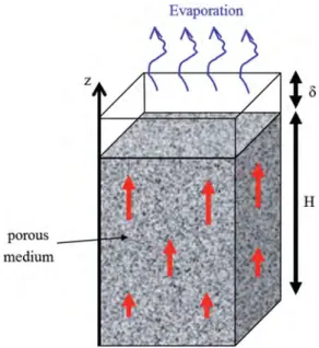
As sketched in Fig.1, we consider a typical drying situation in which vapor can escape only from the top surface of the sample. All other surfaces are sealed. The vertical distribution of liquid saturation during drying depends on the competition between capillary, gravitational, and viscous forces (gener-ated in the liquid by the evaporation process), i.e., Ref.10. For a sufficiently short sample (as typically considered in lab-oratory experiments) and under slow evaporation conditions (such as evaporation with water at room temperature), the drying process is dominated by the capillary forces and the distribution of the saturation during most of the CRP/FRP is essentially uniform in space, i.e., approximately indepen-dent of the vertical coordinate z, e.g., Refs.11and12. This drying regime is referred to as the capillary regime. Under these circumstances, it is easy to show from a mass conser-vation argument that the liquid velocity in the sample during the CRP/FRP varies linearly along the sample height.11This
derivation will be recalled in SectionIIof this paper. It is based on the classical continuum approach for porous media mod-eling, in which the porous medium is regarded as a fictitious continuum.
On the other hand, the capillary regime can be simu-lated using a representation of the void space of the porous medium as a 3D network of pores and by combining inva-sion percolation (IP) rules13with the diffusive vapor transport in the gas phase, i.e., Refs.10and11. The velocity field in the liquid phase can also be computed using such a pore net-work model (details on the pore netnet-work approach are recalled later in the paper). The instantaneous 3D velocity field thus computed can be averaged over the horizontal slices so as to determine the mean velocity in the z direction. In contrast to the velocity field obtained from the continuum description,
FIG. 1. Sketch of considered drying situation. The top region of size δ represents the external mass transfer boundary layer.
the averaged velocity obtained from pore network simula-tions does not vary linearly in the vertical direction, but a step profile is obtained instead. The velocity is typically uniform up to a certain depth within the sample and then vanishes very rapidly as the depth increases, not considering here a thin layer adjacent to the evaporative surface referred to as the edge effect region later in the paper. The main objec-tive of this paper is to reconcile the continuum description of the velocity field during the CRP in the capillary regime with the more detailed information obtained from the pore net-work model. In doing so, we will also reveal new information regarding the velocity field in a slowly drying capillary porous medium.
Somewhat surprisingly at first glance, there is actually no need to compute the velocity field in the liquid phase to pre-dict the saturation distribution during the CRP in the capillary regime, neither in the continuum approach nor in the pore net-work model. Actually, this is fully consistent with the fact that the capillary forces are dominant in this regime. The veloc-ity field becomes important, however, when species such as ions or colloidal particles, for example, are present in the liq-uid, e.g., Refs.11and15–21. The transport of these species during drying and thus their distribution within the porous medium are highly dependent on the velocity field induced in the liquid by the evaporation process. For instance, the occur-rence of salt efflorescence at the surface of a drying porous medium is related to the convective transport of ions toward the evaporative surface by the velocity field, e.g., Refs. 11
and16.
This paper is organized as follows: The derivation of the continuum velocity profile is recalled in SectionII. The pore network (PN) model is presented in SectionIII. Results from PN simulations are presented in SectionIV. The veloc-ity fields from both the PN simulations and the continuum modeling are described in detail in SectionV. A short discus-sion is presented in SectionVIand the conclusion is drawn in SectionVII.
II. VELOCITY FIELD OBTAINED FROM THE CONTINUUM APPROACH
A key feature of the capillary regime is that the satura-tion is spatially uniform during the CRP/FRP. This can be understood from the fact that in this regime the gas invasion resulting from evaporation is controlled by the local cap-illary entry pressure of the constrictions in the pore space and thus by the size of the constrictions (this is made clear in Sec. III). Because the constrictions are distributed ran-domly in the pore space, the probability of invasion is uniform in space, which eventually leads to uniform saturation pro-files. The derivation recalled hereafter takes advantage of this feature.
The average liquid saturation variation during the CRP/FRP can be related to the evaporation flux j from a simple mass balance, j = J A = − m0 A dS dt, (1)
where S is the saturation defined as the ratio of liquid vol-ume to the total pore volvol-ume inside the network, A is the cross sectional surface area of the sample, and m0 is the mass of
liquid saturating the porous medium initially (m0 = AH ρℓε,
with the sample height H, liquid mass density ρℓ, and
porosity ε).
Using similar arguments as in Ref.11, the velocity profile can then be deduced as follows: The one-dimensional local mass balance equation reads
∂S ∂t +
∂
∂z(US) = 0, (2) where S is spatially uniform (capillary regime).
Combining Eq.(1)with Eq.(2)and noting that the velocity is zero at the sample bottom (at z = 0) leads to express the velocity profile as U(z) = A j Sm0z = j εS ρℓ z H. (3)
Note that U represents the average velocity in the pores, referred to as the interstitial velocity, and not the filtration (Darcy’s) velocity UD. Recalling that
UD= εSU, (4) we obtain UD(z) = j ρℓ z H. (5)
Hence the interstitial velocity (as well as the Darcy velocity) varies linearly along the height of sample, is maximum at the evaporative surface (where U(H) = εSρj ℓ and UD(H) =
j
ρℓ),
and vanishes at z = 0. While the filtration velocity does not vary in time during the CRP, the interstitial velocity increases as a function of time at a given location since the saturation S decreases as a function of time.
III. COMPUTATION OF THE VELOCITY FIELD IN PORE NETWORK SIMULATIONS
The pore network modeling is a mesoscale approach based on the representation of the pore space as a network of pore
bodies connected by throat constrictions. The pore network used in this paper is a three-dimensional regular cubic lat-tice of pores and throats based on the work presented in Ref.22. The distance a between the centers of two adjacent pores on the mesh is uniform and called the lattice spac-ing. Throats are cylindrical tubes whereas pores are volume-less computational nodes located at the intersection of the throats.
The throat radii rt are sampled from a normal
distribu-tion with a given mean and standard deviadistribu-tion (as specified in TableIfor our simulations). Evaporation occurs at the top of the network, whereas the bottom is sealed. Periodic boundary conditions are imposed on the lateral faces. An invasion capil-lary pressure threshold is associated with each throat according to Laplace’s law
pcth=2γ cos θr
t
, (6)
where γ is the surface tension and θ is the equilibrium contact angle (which is assumed constant in space and sufficiently smaller than 90◦ for the IP algorithm to apply, see Ref. 23
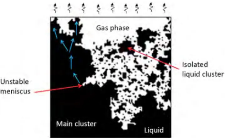
for more details regarding the IP algorithm depending on the contact angle). As discussed in Ref.10, the capillary regime of drying (negligible impact of viscosity and gravity forces on the phase distribution during drying) can be simulated using a pore network model with the algorithm described in Ref.14. In addition to the IP rules and the diffusive transport of the vapor, this algorithm includes the formation of liquid clusters24 as well as isolated liquid throats (see Fig. 3). A liquid cluster is a set of liquid pores interconnected by liq-uid throats. The PN drying algorithm can be summarized as follows:14
1. Every liquid cluster and isolated liquid throat present in the network is identified.
2. The interfacial throat (which contains a meniscus) con-nected to the already invaded region with the low-est threshold capillary pressure is identified for each cluster.
3. The evaporation rate at the boundary of each cluster and isolated liquid throat is computed.
4. For each cluster, the mass loss according to the evapora-tion rate determined in step 3 is assigned to the interfacial throat identified in step 2.
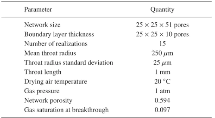
TABLE I. Characteristics of PN drying simulations. Parameter Quantity Network size 25 × 25 × 51 pores Boundary layer thickness 25 × 25 × 10 pores Number of realizations 15 Mean throat radius 250 µm Throat radius standard deviation 25 µm Throat length 1 mm Drying air temperature 20◦C Gas pressure 1 atm Network porosity 0.594 Gas saturation at breakthrough 0.097
5. The throat eventually fully invaded is the first one to be completely drained among the interfacial throats selected in step 2 and the isolated liquid throats.
6. The phase distribution within the network is updated. The gas phase is a binary mixture consisting of the liq-uid vapor and of an inert component. The evaporation rates (step 3) are determined from the computation of the vapor par-tial pressures in the gas-filled region of the network, assuming that the vapor transport is driven by diffusion in the gaseous pore space. The method for computing the vapor diffusion problem on a cubic network is similar to a classical finite dif-ference or finite volume method used to solve the diffusion equation on a regular grid, see Ref.22for more details. As also explained in Ref.22and sketched in Fig.2, additional computational nodes are located in a purely gaseous diffusive layer adjacent to the evaporative surface of the pore network, where only gas diffusion is considered. This external layer rep-resents the external mass transfer boundary layer and is used to impose the difference in vapor partial pressure driving the dry-ing process. As sketched in Fig.2, the number of nodes in the mass transfer boundary layer in the z direction is denoted by NBL.
As can be seen, the liquid viscosity is not a parameter in this drying algorithm. This is consistent with the fact that we are interested in the capillary regime. In this regime, the evolution of the phase distribution during drying is essentially seen as a succession of quasi-static capillary equilibria. The passage from one equilibrium configuration to the next is a very rapid event, referred to as a (global) Haines jump, e.g., Ref.25, which corresponds to the full invasion of a single throat by the gas phase in our model. During the Haines jump, viscous and even inertial effects are not negligible.26 The time scale of the very rapid events corresponding to Haines jump is not resolved. It is assumed that these phenomena do not affect the successive equilibrium fluid configurations obtained by using
FIG. 2. Sketch of a 3D cubic pore network with the gas-diffusion boundary layer on top.
purely quasi-static invasion rules, which is in accordance with experimental observations in model systems, e.g., Refs. 24
and27.
The fact that the velocity generated in the liquid during the drying process has a negligible influence on the time-evolution of the phase distribution does not mean that there is no veloc-ity (in a quasi-static equilibrium configuration). The velocveloc-ity field originates from the so-called pumping effect to the stable menisci at the periphery of each liquid cluster. The pumping effect is schematically illustrated in Fig.3. Consider a stable meniscus, i.e., a meniscus which is not located at the entrance of the largest interfacial throat along the periphery of the clus-ter to which this meniscus belongs. For the meniscus to be stable there must be a liquid flow rate toward this meniscus compensating the evaporation rate from this meniscus. There-fore, a flow is induced in each cluster from the unstable menisci toward the stable menisci. This is called the pumping effect. In the limit of the capillary regime considered here, there is only one throat containing an unstable meniscus in each clus-ter, which is the interfacial throat with the largest radius. The method to compute this flow from unstable to stable menisci within each cluster is as follows: The volumetric flow rate between two liquid pores i and j in a cluster is expressed using Poiseuille’s law as
qij= gij
µ∆Pij, (7) where µ is the liquid dynamic viscosity and ∆Pij = Pi−Pjis
the pressure difference between pores i and j; gijis the
hydra-ulic conductance of the channel connecting the pores i and j,
gij= π rt4,ij
8a . (8)
Expressing the mass conservation at each liquid pore of each cluster,
6
X
j=1
qij= 0, (9)
then yields a linear system which is solved numerically for the pressure in each pore of each cluster. To this end, bound-ary conditions must be specified. At a throat containing a
FIG. 3. Sketch of the pumping effect. The liquid is pumped by capillary action from the region of the unstable meniscus toward the region with high evaporation rates. The liquid motion resulting from the pumping effect is schematically represented by blue arrows.
stable meniscus, the flow rate from the adjacent liquid pore compensates the evaporation rate Jsm from this meniscus.
Thus
qsm=Jρsm
ℓ
, (10)
where Jsm is computed from the numerical solution of the
vapor diffusive transport problem in the gas region of the network. The pressure in the liquid pore um adjacent to the unstable meniscus is fixed for simplicity, assuming Pum= Patm,
where Patm is the gas phase total pressure, which is constant
throughout the gas phase. One should realize that the flow rate computed in each channel is actually independent of µ and Patm. However, a too low viscosity can lead to
numeri-cal problems whereas a too high viscosity is physinumeri-cally not consistent with the assumption that there is only one mov-ing meniscus in a given cluster (this, though, has no impact as long as the identification of the moving meniscus is based on the largest throat IP rule). These channel flow rates are computed from the pressure field using Eq. (7). Then the average velocity in each liquid channel can be determined as
¯uij= qij
π r2tij. (11) Once the flow rates are determined in each liquid channel, the flow rate through each horizontal slice k of the network is computed as Qk= n X m=1 qm, (12)
where n is the number of vertical liquid throats considered in the x-y plane. The filtration velocity in the z direction is then determined as
UDk=
Qk
A, (13)
where A is the cross sectional area of the network.
As illustrated for a piece of a 2D vertical slice of the network in Fig. 4, one can distinguish four types of verti-cal throats: liquid throats between two liquid pores, gaseous
FIG. 4. Illustration of the various types of throats present in the network during drying.
throats between two gaseous pores, isolated liquid throats (marked in red in Fig.4), and cluster liquid throats contain-ing a meniscus. The latter type is referred to as the interfacial throats of a liquid cluster. Three of the latter are indicated with white arrows in Fig.4. The filtration velocity is computed con-sidering only the throats belonging to a liquid cluster, namely, the liquid throats and the interfacial throats. There is no liq-uid flow rate computed in the isolated liqliq-uid throats. For a given cluster, the biggest interfacial throat is the one contain-ing the movcontain-ing meniscus. The mass flow rate in this throat is the sum of the evaporation rates from all stable menisci of the considered cluster. Note also that the flow rate in a vertical liquid throat (liquid or interfacial) is counted posi-tive if the velocity is upward and negaposi-tive if the velocity is downward.
As in Refs.28and29, we define as the main cluster (mc), the biggest liquid cluster connected to the network top surface. As a result, the filtration velocity can be decomposed into two contributions, corresponding respectively to the main cluster and the other clusters (referred to as the isolated clusters (ic)), UD= UDmc+ UDic. (14)
The computation of each component is similar to UD, Eq.(13),
decomposing Qkinto Qk= Qmck+ Qick.The interstitial
veloc-ity cannot be readily deduced from the classical formula Uk = UεDkSk, where ε is the network porosity and Sk is the
slice saturation (see below), because we are interested only in the vertical component of the interstitial velocity. A simple method to compute Ukis
Uk =AQk
wk
, (15)
where Awk is the sum of the cross section areas of the liquid
throats in slice k.
It is also interesting to determine the saturation Skin each
slice of the network. A horizontal slice is defined as an x-y plane of pores and horizontal throats plus half of the vertical throats connected to this plane. The liquid saturation Sk in
each horizontal slice of the network is computed by summing up the liquid volume contained in each throat in slice k and dividing this liquid volume by the total pore space volume in slice k.
IV. PORE NETWORK SIMULATION RESULTS
Pore network drying simulations are performed for 15 realizations on a network initially saturated with water. The main characteristics used in this series of simulations are shown in TableI.
A. Drying curves
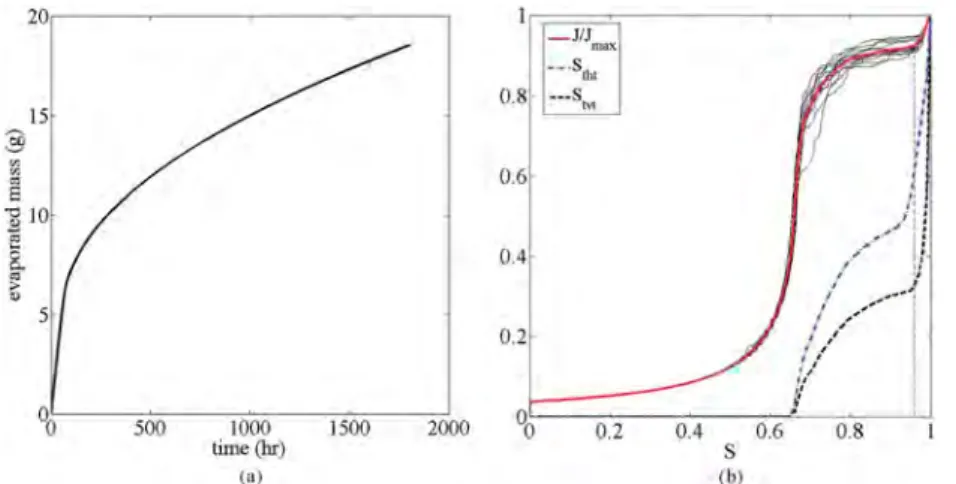
The drying curve obtained from PN simulations aver-aged over 15 realizations is shown in Fig. 5. In order to ensure that the uncertainty in the pore structure results in comparable results, several simulation runs were carried out (Fig.5(b)). The mean standard deviation of individual normal-ized drying rate curves from the normalnormal-ized average drying rate curve over the CRP/FRP is 0.0238 ± (7.1 × 10☞5). There are some differences between this drying rate curve and the typical drying rate curve for the capillary-dominated regime considered in the classical literature, e.g., Ref. 8. The first difference is the decrease in evaporation rate right from the beginning of the drying process, similarly as in previous dry-ing PN simulations, e.g., Refs. 28 and 29. This immediate drop is due to the invasion of surface pores during the very first phase of drying until the gas phase “breakthrough (BT),” i.e., until the gas phase reaches the bottom of the sample for the first time. From percolation theory,30we know that the gas phase saturation in a cubic system with edge length L scales like
SgBT ∝LDf−D (16)
at breakthrough, where D is the space dimension (D = 3), Df is the fractal dimension of the percolation cluster (Df
= 2.52, in 3D), and L is the system size (L = H ≈ Nza) for
our network model. Thus SgBT ∝ L−0.48for 3D systems. As
a result, the gas saturation at breakthrough is very small in a large network, i.e., a typical porous medium sample. This explains why this very first phase cannot be seen in exper-iments, because the corresponding evaporated mass is actu-ally very small compared to the total mass of liquid initiactu-ally present in the sample. Conversely, the relative importance of this phase in our simulations can be related to a finite size effect.
FIG. 5. Drying curves obtained from PN simulations: (a) the average evapo-rated liquid mass as a function of time, (b) the average normalized evaporation rate (red curve), the normalized evap-oration rate for each realization (solid black curves), the average saturation of top vertical throats (dashed black curve), and the average saturation of top hori-zontal throats (blue dashed curve), for capillary-dominated drying. The aver-age curves are obtained considering 15 realizations.
This very first phase is further illustrated by looking at the average saturation of the top vertical throats (Stvt) versus
network saturation (Fig.5). As can be seen, the sharp decrease in the average saturation of top vertical throats is followed by a drop in the evaporation rate during this phase. This also holds for the saturation of top horizontal throats (Stht). One
can refer to Fig. 2 for the definition of top vertical throats and top horizontal throats. As can be seen, the decrease in drying rate occurring in this very first phase affects the dry-ing rate durdry-ing the CRP, which starts at the end of this initial phase. The evaporation rate is actually not perfectly constant but varies weakly during the “constant” rate period. This has also been observed in previous pore network simulations, e.g., Refs.28and29. Compared to classical experimental results, the CRP obtained from the simulations is quite short (the satu-ration range corresponding to the CRP is much narrower than in the experiments). Several factors explain this difference: First, the irreducible saturation, i.e., the saturation for which the liquid phase is no longer connected over a distance compa-rable to the system size, is quite high in our system (Sirr≈0.65)
compared to a random packing of monodisperse spherical par-ticles (Sirr≈0.1, Ref.31) or the fired clay brick considered in
Ref.12(Sirr< 0.1). This has to do with the coordination
num-ber of our network (each pore is connected to 6 neighbor pores) which is low compared to the average coordination number in real systems. Second, the fact that the pores are volume-less and thus that all the pore space volume is in the channels (throats) leads to a greater irreducible saturation (Sirr≈0.65 vs
Sirr≈0.45 for the network considered in Ref.28for instance).
The high irreducible saturation favors an earlier end of the CRP owing to an earlier fragmentation of the liquid phase into iso-lated clusters. Third, the external mass transfer boundary layer thickness measured in lattice spacing units is quite small in our simulations (δ = 10a) compared to experiments with real sys-tems (for example, δ = 100a for a typical convective boundary layer of 1 mm over a micrometer-sized porous medium char-acterized by a mean distance of 10 µm between adjacent pores). This favors a greater impact on the drying kinetics of changes in the throat saturations near the top surface of the network.
Although the CRP is shorter, the key point is to obtain a quasi-CRP from our simulations. The smooth decrease in the drying rate during the CRP becomes sharper during the FRP. Then the RFP starts a little after the local saturations inside the network approach the irreducible saturation (around 0.65), at which the conductivity of the liquid phase across the whole network is lost.
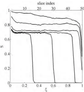
B. Horizontal slice-averaged saturation profiles
The average slice saturation inside the pore network for different network saturations is shown in Fig.6. These results are in quite good qualitative agreement with the experimen-tal profiles measured by nuclear magnetic resonance (NMR) reported, for example, in Ref.12(see Fig.2(a)in this reference) if one takes into account that (1) the irreducible saturation is much higher with our cubic network as explained previously and (2) the initial phase up to the gas breakthrough which is, as explained, difficult to observe in experiments. This phase corresponds to the topmost profile in Fig.6characterized by
FIG. 6. Saturation profiles of capillary-dominated drying obtained from PN simulations and averaged over 15 realizations. From the top, profiles corre-sponding to the network saturation 0.9, 0.8, 0.7, 0.6, 0.4, and 0.2, respectively; ξ = z/H. The evaporative top surface of the network is located at ξ = 1.
a liquid saturation which increases with the depth. If one dis-regards this first profile, an almost uniform saturation profile for total network saturations greater than the irreducible satu-ration (S = 0.65) is observed, similarly as in the experiments. One can observe, however, a sharp drop in saturation at posi-tions near the evaporative surface. This was also observed in previous PN simulations, e.g., Refs.28and29, and even more interestingly in the experimental profiles obtained by NMR, e.g., Refs.12and32. This sharp drop is due to the preferential invasion in the top horizontal and vertical throats (Stht, Stvt),
as shown in Fig.5. The emptying of the top vertical throats leads to the formation of many isolated horizontal single liquid throats just below the top pores. These isolated single liquid throats are disconnected from the body of the liquid phase inside the network, and therefore they empty quickly, leading to a lower saturation near the top compared to deeper inside the network. Similarly as in the PN simulations reported in Ref. 28 (see Fig. 5 in this reference) over a network twice as large, this edge effect actually affects about 3-4 first rows of pores. It is, however, unclear how the extent of this near surface region will change with the network size. The fact that the saturation edge effect is also observed in experiments suggests that the size of the region affected by the satura-tion edge effect increases with the network size. This edge effect has clearly an impact on the drying kinetics as shown in Fig.5(b).
C. Liquid cluster formation
As mentioned earlier and quantitatively illustrated for our pore network in Fig.7, liquid clusters form during dry-ing. The number of clusters increases during the CRP/FRP until the main cluster detaches from the top surface of the network. This event is referred to as the main cluster discon-nection (MCD).28,29The number of clusters connected to the
top surface of the network is quite low, however, varying typ-ically between 1 and 2 during the CRP/FRP. Thus, the liquid
FIG. 7. Number of liquid clusters present in the pore network and number of liquid clusters connected to the top surface as a function of overall saturation. The data are averaged over 15 realizations.
phase fragmentation, i.e., the formation of clusters, takes place mostly inside the network. The results reported in Fig.7also give insights into the edge effect since there are clusters con-nected to the top surface formed during the short phase before breakthrough (BT). These clusters evaporate during this initial phase, which leads to the formation of dry pockets connected to the surface. Fig.8presents similar results when the isolated liquid throats are taken into account. The comparison between
FIG. 8. Number of liquid clusters present in the pore network plus the number of isolated menisci (im) and number of liquid clusters plus isolated menisci connected to the top surface as a function of overall saturation. The data are averaged over 15 realizations.
Figs. 7 and8 shows that many isolated liquid throats form within the network. The isolated throats connected to the sur-face rapidly evaporate during the initial short phase before BT. The formation and evaporation of those throats con-tribute to the edge effect and to the modification of the liquid distribution right at the surface between the initial distribution (all the vertical throats attached at the surface are
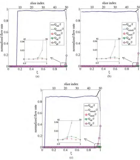
FIG. 9. Variation of contributions to
Qm(Eq. (17)) as a function of z cor-responding to the network saturation 0.9 (a), 0.8 (b), and 0.7 (c); Qmmck = ρℓUDmckA; Qmick= ρℓUDickA; J is the evaporation rate corresponding to each global saturation.
FIG. 10. Example of slice-averaged velocity profiles: (a) profiles corre-sponding to the data shown in Fig.9
(moving meniscus in the lower part of the network), (b) velocity profiles for comparable saturations as in Fig.10(a)
but with a moving meniscus in the main cluster located closer to the network top surface (ξ = 1).
filled with liquid) and the distribution when the CRP starts (some throats are empty).
D. Mass flow rate partition
To obtain first insights into the slice-averaged velocity field in the network, we compute the total mass flux Qm
reach-ing the top plane of each slice from below. It can be expressed as
Qmk= ρℓUDmckA + ρℓUDickA + Qgk+ Qitk, (17)
where Qgkis the diffusive mass flow rate between the
horizon-tal planes k and limiting slice k + 1 (see Fig.4) through the ver-tical gaseous throats connecting the two planes, shown in grey in Fig.4. Qitkis the evaporation rate from the top menisci of the
isolated liquid throats (marked in white in Fig.4) located in the slice.
The variation of each contribution to Qmas a function of z
is shown in Fig.9for three different overall saturations in the CRP/FRP for cases where the moving meniscus in the main cluster is not very far from the network bottom.
As can be seen from Fig.9, one must distinguish the thin edge effect region from the rest of the network, referred to as the bulk in what follows. In the bulk, the transport in the gas phase is completely negligible and there is no contribution of the isolated clusters to the liquid transport. The evapora-tion from those clusters is screened and therefore negligible. Indeed, the pore network simulations indicate that the vapor partial pressure in the pores of the network invaded by the gas phase is very close to the saturation pressure (equilib-rium vapor partial pressure imposed at the surface of each meniscus). This is consistent with the classical description, e.g., Ref.8, considering that the transport of vapor is negligi-ble within the porous medium compared to the transport in the liquid phase during the CRP. The transport in the bulk there-fore occurs in the liquid phase and through the main cluster, which is connected to the top surface of the network. The sit-uation is more complex in the edge effect region where the contribution of isolated clusters, although quite weak, is not completely negligible. However, the most significant change is that the transport in the gas phase is noticeable in this region. Because of the edge effect and the contribution of the gas diffusive transport, the filtration velocity is not simply given
by UD= J/ (A ρℓ) (which is the continuum model prediction),
but actually UD< J/ (A ρℓ) in the bulk and decreasing within
the edge effect region in the direction of the network top surface.
E. Slice-averaged velocity profiles
As illustrated in Fig. 10, horizontal slice-averaging of the instantaneous velocity field in the network produces step velocity profiles which are markedly different from the linear profile predicted by continuum models (Eq.(5)).
The step velocity profile can be explained as follows: As shown in Section IV D, there is no evaporation inside the network. Thus, the vapor transport is negligible within the porous medium compared to the transport in the liquid phase. Thus evaporation takes place only from the menisci close to the porous medium surface, namely, within the edge effect region (as illustrated in Fig.9). The physical picture is then as sketched in Fig.11.
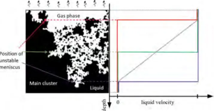
Based on the results presented in Sec.IV D, the liquid phase is essentially moving in a single cluster, referred to as the main cluster. Thus, we only consider this cluster. Let kum
be the plane in which the moving meniscus in the main cluster is located at the time considered. Since there is no evapo-ration within the porous medium but only at its surface, the filtration velocity is actually different from zero only in the planes located above the plane kum. Furthermore, since again
FIG. 11. A 2D schematic phase distribution in a porous sample during capillary-dominated drying (left picture) and three velocity profiles of sin-gle invasion events corresponding to three different positions of the unstable meniscus and their average (in grey) (right picture).
the internal evaporation is negligible, the filtration velocity is actually uniform and constant in the planes located above the plane kum. As a result, the PNM filtration velocity profiles are
given by
UDz=
J A ρℓ
for kum< k ≤ N and UDz= 0 for 1 ≤ k < kum.
(18)
V. RECONCILING THE CONTINUUM AND PNM VELOCITY FIELDS
The vertical filtration velocity profile deduced from the continuum approach (Eq.(5), the velocity increases linearly from bottom to top) is markedly different from the one obtained with the PNM model (Eq.(18), step profile).
To reconcile the two approaches, an approximation is to consider that the unstable meniscus position can be located in any horizontal plane with equal probability. To this aim, a fraction of moving menisci in the main cluster in each slice is obtained by averaging over fifteen realizations. The procedure to obtain these results is as follows: First, for each realization at each position the fraction of invasions in the main cluster is obtained. 1000 invasions in all clusters and isolated throats at each overall saturation are considered, and then the num-ber of invasions in the main cluster in each plane is divided by 1000. The same method is applied to other realizations. Second, for each overall saturation, in each position all the fractions of invasions in the main cluster, obtained from 15 realizations, are summed up and then divided by 15. As can be
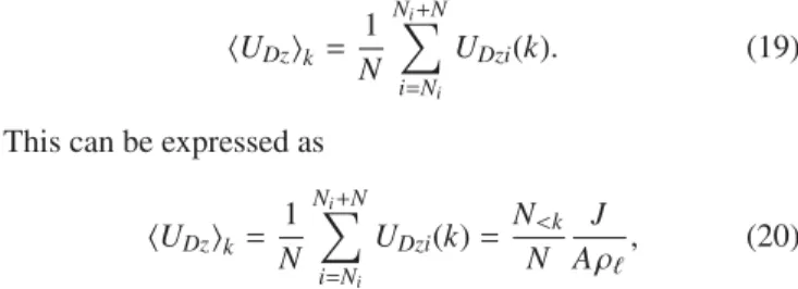
seen from Fig.12, this is only a fair approximation. Accord-ing to the PN approach, the velocity field varies from one to the next channel invasion event in the main cluster. The next step is then to average the PN velocity field over a certain number of invasion events N, which is equivalent to a time averaging, hUDzik= 1 N NXi+N i=Ni UDzi(k). (19)
This can be expressed as
hUDzik= 1 N NXi+N i=Ni UDzi(k) = N<k N J A ρℓ , (20)
where N<k is the number of invasions (out of N) for which
the unstable meniscus is located below the plane k. HenceN<k N
can be interpreted as the probability that the unstable menis-cus is located below the plane k. Assuming that the unstable meniscus can be located in any horizontal plane with equal probability, N<k N ≈ (k − 1) Nz , (21)
where Nz is the total number of horizontal planes in the
network. Combining Eq.(20)with Eq.(21)yields
hUDzik= (k − 1)a Nza J A ρℓ ≈zk L J A ρℓ , (22)
which is a discrete version of Eq.(5).
FIG. 12. Fraction of moving menisci in the main cluster in each slice obtained by averaging over fifteen realizations.
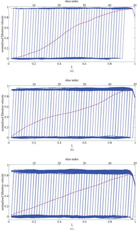
Thus, the filtration velocity as well as the interstitial velocity of the continuum approach can be interpreted as a time-averaged velocity of the PN approach. This is illustrated in Fig. 13 from the numerical PN simulations. In Fig. 13, instantaneous step velocity profiles corresponding to various single invasions are needed to obtain a quasi-linear average velocity profile for network saturations 0.9, 0.8, and 0.7. The blue lines show the step velocity profiles associated with each single invasion. The average velocity profile is shown in purple. The number of invasions per realization needed to obtain the quasi-linear average velocity profiles for network saturations 0.9, 0.8, and 0.7 are on average 751, 761, and 806, respectively.
The procedure to obtain the average velocity profiles is actually the following: Overall saturation intervals are defined, between S + 0.05 and S☞ 0.05. These intervals are considered to obtain the average velocity profiles for each realization at each corresponding overall saturation. Then for each overall saturation, averages are computed among all velocity profiles obtained from all realizations (summing up 15 values of veloc-ity at each position obtained from 15 realizations and dividing it by 15). For each realization, the number of invasions (in all clusters and isolated throats) in the three aforementioned overall saturation intervals is counted and summed up over all realizations. Then these 3 numbers are divided by 15 to give the average number of invasions at each overall saturation, which
FIG. 13. Normalized step filtration velocity profiles induced by single invasions (blue lines) for a single realization in the capillary-dominated regime for network saturations 0.9 (a), 0.8 (b), and 0.7 (c) obtained from PN simulation. The average velocity profile between all invasions and realizations is also shown in purple. The velocities are normalized by AρJ
ℓ, where J is the
evaporation rate corresponding to each overall saturation.
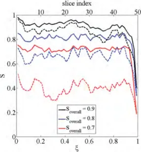
FIG. 14. Normalized velocity profiles in the capillary-dominated regime obtained from time-averaging of the step single invasion velocity profiles over all realizations for three different network saturations. The velocities are normalized by AρJ
ℓ, where J is the evaporation rate corresponding to each
overall saturation.
are used to produce the curves in Fig.13(purple curve). It can be also mentioned that the numbers of invasions corresponding to each overall saturation interval for different realizations are very close to each other (plus minus 10 invasions difference between realizations).
The time-averaged velocity profiles thus obtained are shown together in Fig. 14. In addition to obtaining a quasi-linear variation consistent with the velocity profiles obtained within the continuum framework, Fig.14illustrates the impact of the edge effect characterized by a drop in the velocity in the edge effect region. This drop is not predicted within the framework of the continuum approach.
The fact that the average profiles are not perfectly linear is consistent with the histograms shown in Fig.12. For example, for S = 0.8, one can see that the slope of the velocity profile at the bottom (ξ < ∼0.2) is greater than for the other two velocity profiles. This is consistent with the fact that the histogram (Fig.12) indicates that there are many invasions happening at those positions. Also, the slope of the filtration velocity profile in Fig.14decreases in the interval (∼0.2 < ξ < ∼0.6). This is consistent with the histogram in Fig.12indicating that there are not many invasions happening within this interval (compared to the region ξ < ∼0.2). Finally, an increase in the slope of the average filtration velocity is again observed in the region ξ > ∼0.7, which is due to the presence of many moving menisci in this part.
VI. DISCUSSION
A condition for obtaining almost perfectly linear aver-aged velocity profiles, as for the case S = 0.7 in Fig.14, is that the histogram is quasi-uniform (equal probability in the distribution of moving menisci along the vertical). Consis-tently with the quasi-linear velocity profile obtained for S = 0.7, the histogram for this saturation in Fig.12is the one closest to a uniform probability distribution. We surmise that more
uniform histograms would be obtained during the CRP/FRP by considering larger networks or a greater number of real-izations. We also note that the case S = 0.9 is different since this saturation corresponds to the very first phase before break-through, where the saturation profile is not uniform. Although it would be desirable to repeat the work considering larger net-works, we believe that the results obtained from our relatively small network provide a clear and convincing interpretation of the velocity field when the liquid phase is connected to the top surface of the porous medium (CRP and FRP) in the capillary regime.
One interesting outcome is that the velocity induced in the liquid phase as a result of the evaporation process essen-tially takes place in the main cluster. As illustrated in Fig.15, a noticeable fraction of the liquid phase does not belong to the main cluster. Thus, there are liquid regions within the network completely inactive in terms of convective transport, suggest-ing that it would be interestsuggest-ing to clearly distsuggest-inguish the main cluster from the other liquid clusters when analyzing the trans-port of dissolved species or particles during drying. This is in contrast to the classical continuum approach which uses a single variable, i.e., the saturation, to characterize the local presence of the liquid phase, without distinguishing between the saturation corresponding to the main cluster and the satu-ration associated with the other clusters. This suggests that it would be interesting to develop new continuum models mak-ing explicitly the distinction between the movmak-ing liquid phase and the liquid phase at rest.
Although the analysis leads to consistent results (except in the edge effect region) between the classical continuum approach and the PN simulations as far as the (averaged) velocity field is concerned, the (instantaneous) velocity field is probably still more complex. For instance, we argue that the Haines jumps have little impact on the liquid-gas distribu-tions within the pore space, which essentially correspond to quasi-static distributions. However, it is unclear whether the
FIG. 15. Saturation profiles for a single realization, considering all clusters and all isolated liquid throats (solid lines) and only the main cluster (dashed lines) for overall saturations 0.9, 0.8, and 0.7.
Haines jumps have an impact on the convective transport of a species.
Also, we have not taken into account the possible presence of liquid films. It is relatively well established that liquid films can have a great impact on the drying process, e.g., Refs.33
and34. This actually depends on the wettability properties of the three phases:35The lower the contact angle is, the more likely the film has a significant impact. However, based on the existing PN models of drying with films, e.g., Refs.35–37, the presence of the films should not change the main results presented in the paper except that the CRP computed with the PNM would be longer when liquid films are added to the model.
VII. CONCLUSIONS
The velocity field induced in the liquid phase during dry-ing in the capillary regime was analyzed. The main result was that the velocity predicted from the classical continuum approach can be interpreted as a temporally and spatially aver-aged velocity. While it is traditional to consider the continuum (Darcy)-scale velocity as a spatial average, i.e., Ref.38, it is less common to combine spatial and temporal averaging to obtain upscaled descriptions. This is done, for example, in the upscaling of turbulent flows in porous media, e.g., Ref.39. In the case of two-phase flow, the formal upscaling, e.g., Ref.40, is typically performed assuming quasi-static distributions of the fluids at the REV scale without any time-averaging pro-cedure since all menisci are actually considered as static. In this context, our results suggest that the classical Darcy-scale equations used to describe the drying process in the capillary regime could be rigorously derived combining space and time averages.
Our results also suggest that one of the key issues in the modeling and analysis of drying is the edge effect region. Since drying is controlled by what happens at the surface during the CRP/FRP, this region is of key importance. The consequence for the modeling of drying within the continuum framework would be to develop a specific modeling for this region so as to take into account adequately the impact of this region on evap-oration. It is well known that the interfacial region between a porous medium and a free fluid deserves special attention in the somewhat simpler cases where there is a single fluid and no phase change, e.g., Refs.41and42. In that respect, it makes sense that this must also be the case for the significantly more complex drying situation.
Finally, our results also open up a route for better anal-ysis of the transport of species (ions, particles) that can be present in the liquid phase during drying43owing to the fun-damentally different structure of the instantaneous spatially averaged velocity field compared to the velocity field obtained from the continuum model. In this respect, it would be inter-esting to compare pore network simulations and continuum model-based predictions in the same spirit as the velocity field analysis presented here. Also, our results suggest that making a clear distinction between the convective active liquid phase (corresponding to the main cluster) and the non-active liquid phase (corresponding to the isolated liquid clusters) could be instrumental for developing better species transport models.
ACKNOWLEDGMENTS
This work was financed by the German Research Foun-dation (DFG) in the frame of Graduate School 1554 “Micro-Macro-Interactions in Structured Media and Particulate Sys-tems.”
1W. Brutsaert, Evaporation into the Atmosphere: Theory, History and Applications(Springer, 1982).
2A. S. Mujumdar, Handbook of Industrial Drying, 4th ed. (CRC Press, 2015). 3C. K. Ho and K. K. Udell, “An experimental investigation of air venting of
volatile liquid hydrocarbon mixtures from homogeneous and heterogeneous porous media,”J. Contam. Hydrol.11(3-4), 291–316 (1992).
4E. F. M´edici and J. S. Allen, “Evaporation, two phase flow, and thermal
transport in porous media with application to low-temperature fuel cells,”
Int. J. Heat Mass Transfer65, 779–788 (2013).
5K. H. Le, A. Kharaghani, C. Kirsch, and E. Tsotsas, “Pore network
simula-tions of heat and mass transfer inside an unsaturated capillary porous wick in the dry-out regime,”Transp. Porous Media114, 623–678 (2016).
6C. Duan, R. Karnik, M.-C. Lu, and A. Majumdar, “Evaporation-induced
cavitation in nanofluidic channels,”Proc. Natl. Acad. Sci. U. S. A.109(10), 3688–3693 (2012).
7O. Vincent, D. A. Sessoms, E. J. Huber, J. Guioth, and A. D. Stroock,
“Dry-ing by cavitation and poroelastic relaxations in porous media with macro-scopic pores connected by nanoscale throats,”Phys. Rev. Lett.113(13), 134501 (2014).
8J. Van Brakel, “Mass transfer in convective drying,” in Advances in Drying,
edited by A. S. Mujumdar (Hemisphere, New-York, 1980), pp. 217–267.
9P. Coussot, “Scaling approach of the convective drying of a porous medium,” Eur. Phys. J. B15, 557–566 (2000).
10M. Prat, “Recent advances in pore-scale models for drying of porous media,”
Chem. Eng. J.86, 153–164 (2002).
11H. P. Huinink, L. Pel, and M. A. J. Michels, “How ions distribute in a drying
porous medium: A simple model,”Phys. Fluids14(4), 1389–1395 (2002).
12S. Gupta, H. Huinink, M. Prat, L. Pel, and K. Kopinga, “Paradoxical drying
due to salt crystallization,”Chem. Eng. Sci.109, 204–211 (2014).
13D. Wilkinson and J. F. Willemsen, “Invasion percolation: A new form of
percolation theory,”J. Phys. A: Math. Gen.16, 3365–3376 (1983).
14M. Prat, “Percolation model of drying under isothermal conditions in porous
media,”Int. J. Multiphase Flow19, 691–704 (1993).
15L. Guglielmini, A. Gontcharov, A. J. Aldykiewicz, and H. A. Stone,
“Dry-ing of salt solutions in porous materials: Intermediate-time dynamics and efflorescence,”Phys. Fluids20, 077101 (2008).
16H. Eloukabi, N. Sghaier, S. Ben Nasrallah, and M. Prat, “Experimental
study of the effect of sodium chloride on drying of porous media: The crusty—Patchy efflorescence transition,”Int. J. Heat Mass Transfer56, 80– 93 (2013).
17F. Hidri, N. Sghaier, H. Eloukabi, M. Prat, and S. Ben Nasrallah, “Porous
medium coffee ring effect and other factors affecting the first crystallisation time of sodium chloride at the surface of a drying porous medium,”Phys. Fluids25(12), 127101 (2013).
18M. N. Rad, N. Shokri, and M. Sahimi, “Pore-scale dynamics of salt
precipitation in drying porous media,”Phys. Rev. E88, 032404 (2013).
19J. Desarnaud, H. Derluyn, L. Molari, S. de Miranda, V. Cnudde, and
N. Shahidzadeh, “Drying of salt contaminated porous media: Effect of primary and secondary nucleation,”J. Appl. Phys.118(11), 114901 (2015).
20E. Keita, P. Faure, S. Rodts, and P. Coussot, “MRI evidence for a
receding-front effect in drying porous media,”Phys. Rev. E87, 062303 (2013).
21E. Keita, T. E. Kodger, P. Faure, S. Rodts, D. A. Weitz, and P. Coussot,
“Water retention against drying with soft-particle suspensions in porous media,”Phys. Rev. E94, 033104 (2016).
22T. Metzger, E. Tsotsas, and M. Prat, “Pore network models: A powerful tool
to study drying at the pore level and understand the influence of structure on drying kinetics,” in Modern Drying Technology, Computational Tools at Different Scales, Vol. 1, edited by A. Mujumdar and E. Tsotsas (Wiley, 2007).
23M. Cieplak and M. O. Robbins, “Influence of contact angle on quasistatic
fluid invasion of porous media,”Phys. Rev. B41, 11508 (1990).
24J. B. Laurindo and M. Prat, “Numerical and experimental network study
of evaporation in capillary porous media. Phase distributions,”Chem. Eng. Sci.51(23), 5171–5185 (1996).
25R. T. Armstrong and S. Berg, “Interfacial velocities and capillary pressure
26A. Ferrari and I. Lunati, “Inertial effects during irreversible meniscus
reconfiguration in angular pores,”Adv. Water Resour.74, 1–13 (2014).
27M. Jung, M. Brinkmann, R. Seemann, T. Hiller, M. Sanchez de La Lama,
and S. Herminghaus, “Wettability controls slow immiscible displacement through local interfacial instabilities,”Phys. Rev. Fluids1, 074202 (2016).
28Y. Le Bray and M. Prat, “Three dimensional pore network simulation of
drying in capillary porous media,”Int. J. Heat Mass Transfer42, 4207–4224 (1999).
29A. G. Yiotis, I. N. Tsimpanogiannis, A. K. Stubos, and Y. C. Yortsos,
“Pore-network study of the characteristic periods in the drying of porous materials,”J. Colloid Interface Sci.297, 738–748 (2006).
30D. Wilkinson, “Percolation effects in immiscible displacement,” Phys.
Rev. A34(2), 1380–1391 (1986).
31F. A. L. Dullien, C. Zarcone, I. F. Mac Donald, A. Collins, and R. D.
E. Bochard, “The effects of surface roughness on the capillary pressure curves and the heights of capillary rise in glass bead packs,”J. Colloid Interface Sci.127(2), 362 (1989).
32P. Faure and P. Coussot, “Drying of a model soil,”Phys. Rev. E82, 036303
(2010).
33F. Chauvet, P. Duru, S. Geoffroy, and M. Prat, “Three periods of drying of
a single square capillary tube,”Phys. Rev. Lett.103, 124502 (2009).
34A. G. Yiotis, D. Salin, E. S. Tajer, and Y. C. Yortsos, “Drying in porous
media with gravity-stabilized fronts: Experimental results,”Phys. Rev. E 86, 026310 (2012).
35M. Prat, “On the influence of pore shape, contact angle and film flows on
drying of capillary porous media,”Int. J. Heat Mass Transfer50, 1455–1468 (2007).
36A. G. Yiotis, A. G. Boudouvis, A. K. Stubos, I. N. Tsimpanogiannis, and
Y. C. Yortsos, “Effect of liquid films on the isothermal drying of porous media,”Phys. Rev. E68, 037303 (2003).
37N. Vorhauer, Y. J. Wang, A. Kharaghani, E. Tsotsas, and M. Prat, “Drying
with formation of capillary rings in a model porous medium,”Transp. Porous
Media110, 197–223 (2015).
38S. Whitaker, The Method of Volume Averaging (Springer Science & Business
Media, 1998).
39M. de Lemos, Turbulence in Porous Media (Elsevier, 2012).
40S. Whitaker, “Flow in porous media II: The governing equations for
immiscible, two-phase flow,” Transp. Porous Media 1(2), 105–125 (1986).
41J. A. Ochoa-Tapia and S. Whitaker, “Momentum transfer at the
bound-ary between a porous medium and a homogeneous fluid-I. Theoretical development,”Int. J. Heat Mass Transfer38(14), 2635–2646 (1995).
42M. Chandesris and D. Jamet, “Jump conditions and surface-excess quantities
at a fluid/porous interface: A multi-scale approach,”Transp. Porous Media 78(3), 419–438 (2009).
43S. Veran-Tissoires and M. Prat, “Evaporation of a sodium chloride solution
from a saturated porous medium with efflorescence formation,”J. Fluids