1
Uncertainty of stationary and nonstationary models for rainfall frequency analysis
12
3
T.B.M.J. Ouarda1,*, C. Charron1 and A. St-Hilaire1 4
5
1Canada Research Chair in Statistical Hydro-climatology, INRS-ETE, 490 de la Couronne, 6
Quebec City (QC), G1K9A9, Canada 7 8 9 10 *Corresponding author: 11 Email: [email protected] 12 Tel: +1 418 654 3842 13 14 15 16 17 18 July 2019 19 20
2
Abstract 21
The development of nonstationary frequency analysis models is gaining popularity in the field of 22
hydro-climatology. Such models account for nonstationarities related to climate change and 23
climate variability but at the price of added complexity. It has been debated if such models are 24
worth developing considering the increase in uncertainty inherent to more complex models. 25
However, the uncertainty associated to nonstationary models is rarely studied. The objective of 26
this paper is to compare the uncertainties in stationary and nonstationary models based on objective 27
criteria. The study is based on observed rainfall data in the United Arab Emirates (UAE) where 28
strong nonstationarities were observed. In this study, a nonstationary frequency analysis 29
introducing covariates into the distribution parameters was carried out for total and maximum 30
annual rainfalls observed in the UAE. The Generalized Extreme Value (GEV) distribution was 31
used to model annual maximum rainfalls and the gamma (G) distribution was used to model total 32
annual rainfalls. A number of nonstationary models, using time and climate indices as covariates, 33
were developed and compared to classical stationary frequency analysis models. Two climate 34
oscillation patterns having strong impacts on precipitation in the UAE were selected: the Oceanic 35
Niño Index and the Northern Oscillation Index. Results indicate that the inclusion of a climate 36
oscillation index generally improves the fit of the models to the observed data and the inclusion of 37
two covariates generally provides the overall best fits. Uncertainties of estimated quantiles were 38
assessed with confidence intervals computed with the parametric bootstrap method. Results show 39
that for the small sample sizes in this study, the width of the confidence intervals can be very large 40
for extreme nonexceedance probabilities and for the most extreme values of the climate index 41
covariates. The weaknesses of nonstationary models revealed by the bootstrap uncertainties are 42
discussed and words of caution are formulated. 43
3
Keywords 44
Rainfall; Arid-climate; Nonstationary frequency analysis; Teleconnection; Climate oscillation 45
index; parametric bootstrap; uncertainty; United Arab Emirates. 46
4
1. Introduction
47
The presence of nonstationarity in hydro-climatic time series in a context of climate change 48
is commonly accepted. Also, large scale oscillation phenomena modulate climate around the world 49
and impact hydro-climatic variables. In classical frequency analysis models, observations are 50
assumed to be independent and identically distributed (iid). However, these assumptions are not 51
met in the presence of the nonstationarities. Considerable efforts have hence been invested on the 52
development of nonstationary frequency analysis models for hydro-climatic variables. 53
One approach frequently used to deal with nonstationarities in data samples is to introduce 54
covariates into the parameters of the distribution (e.g. Strupczewski at al., 2001; Katz et al., 2002; 55
Khaliq et al., 2006; El Adlouni et al., 2007; Ouarda and El Adlouni, 2011). Covariate and time-56
dependent conditional distributions are then obtained. Such covariates could incorporate whatever 57
drives the variable under study, e.g. trends, cycles or physical variables that can represent 58
atmosphere-ocean patterns (Katz et al., 2002). This approach has gained wide popularity with 59
applications to a large number of hydro-climatic extremes such as rainfall (Thiombiano et al., 60
2017, 2018; Ouarda et al., 2018), floods (Villarini et al., 2009), wind speeds (Hundecha et al., 61
2008), air temperatures (Wang et al., 2013, Ouarda and Charron, 2018) and sea wave heights 62
(Wang and Swail, 2006). 63
The introduction of covariates in the frequency analysis process introduces additional 64
difficulties in the estimation of the parameters of the model. It also introduces an additional stage 65
in the estimation process: Aside from the identification of the appropriate distribution, it is 66
necessary to identify the level of complexity of the dependence relationship between the covariates 67
and the parameters, before proceeding to the estimation process. El Adlouni and Ouarda (2009) 68
5
proposed a procedure based on the birth-death Markov chain Monte Carlo technique which allows 69
combining the identification of the optimal dependence relationship between covariates and 70
parameters, and the estimation process into a single step. 71
There is some debate as to whether nonstationary models provide more reliable estimates in 72
practical applications. Milly et. al. (2008) pleaded for an extensive use of nonstationary models 73
instead of the stationary models for water management in the context of climate change. A number 74
of authors (for instance Lins et al., 2011; Serinaldi and Kilsby, 2015), while recognizing that 75
nonstationarity exists, criticized nonstationary models and claimed that stationary models should 76
not be abandoned. Serinaldi and Kilsby (2015) provided a critical overview of the concepts and 77
methods used in nonstationary frequency analysis. They reported that uncertainty can be very large 78
given the increase in complexity of nonstationary models. They stressed out the importance of a 79
fair comparison of the models through the assessment of sampling uncertainties. Ganguli and 80
Coulibaly (2017) investigated nonstationarities and trends in short-duration precipitation extremes 81
in selected urbanized locations in Southern Ontario, Canada, and indicated that the nonstationarity 82
signature in rainfall extremes does not necessarily imply the use of nonstationary IDFs for design 83
purposes. Ganguli and Coulibaly (2019) used RCP8.5 scenario projections for the same study area 84
and found a significant increase in shorter return levels using both stationary and nonstationary 85
frequency analysis methods and a detectable trend was noted for longer return period estimates. 86
The present work proposes to study the uncertainties associated to stationary and 87
nonstationary models. A comparison of the uncertainties in the estimation of hydro-climatic 88
variables obtained with nonstationary and stationary models is carried out based on observed data. 89
Uncertainties are quantified by the mean of confidence intervals computed by parametric 90
6
bootstrapping. The case study consists in data from three rainfall stations in the United Arab 91
Emirates (UAE), a region characterised by a desert environment and not often studied. 92
The rainfall regime of the UAE was studied in Ouarda et al. (2014). The total annual rainfall, 93
the annual maximum rainfall and the number of rainy days per year were analyzed at a number of 94
relatively long-record meteorological stations. While the analysis of trends performed with the 95
Mann-Kendall test indicated slight downward trends for the annual time series, the application of 96
a multiple change point detection procedure revealed that a shift occurred around 1999 with 97
positive trends for the two subsamples before and after the change point. To cope with the presence 98
of the shift, separate frequency analyses with the data samples before and after the change point 99
can be performed, although this reduces the sample sizes considerably. However, the positive 100
trends detected in the subsamples still violate the iid assumption. 101
Evidence of the influence of climate oscillation patterns on precipitation in the region 102
surrounding the UAE has been established in a few studies. A link between precipitation in Iran 103
and the El Niño Southern Oscillation (ENSO) phenomenon were established by Nazemosadat and 104
Ghasemi (2004), and Dezfuli et al. (2010). Also in Iran, Ghasemi and Khalili (2008) analyzed the 105
relationship between several global atmospheric patterns and winter precipitation, and found that 106
the indices with the strongest impacts are the North Sea-Caspian, the Western Mediterranean 107
Oscillation and the North Atlantic Oscillation (NAO) indices. A link between precipitation in the 108
Middle East and NAO was also shown in Cullen et al. (2002). The relationship betweenrainfall in 109
India and ENSO was established by Krishnamurthy and Goswami (2000), Ashok and Saji (2007), 110
and Dimri (2013), and with Indian Ocean dipole (IOD) by Ashok and Saji (2007). 111
7
Recently, a number of studies have focused on the study of the climate of the UAE. Ouarda 112
et al. (2014) demonstrated the strong impact that the ENSO phenomenon has on precipitation over 113
the UAE. They indicated that the observed change in the precipitation regime around 1999 is also 114
caused by ENSO. Niranjan Kumar and Ouarda (2014) concluded that the major portion of the 115
precipitation variability is influenced by equatorial Pacific sea surface temperatures associated 116
with ENSO. In Chandran et al. (2015), the relation of precipitation in the UAE with several global 117
climate oscillations was investigated using wavelet and crosswavelet analysis. The authors found 118
also that global climate oscillations related to ENSO have a strong impact. According to the same 119
study, other climate oscillations that have important impacts are the IOD and the Pacific Decadal 120
Oscillation (PDO). Naizghi and Ouarda (2017) examined the long-term variability of wind speed 121
in the UAE and its teleconnections with various global climate indices. Wavelet coherence analysis 122
demonstrated that wind speed in the UAE is mainly associated with the NAO, East Atlantic (EA) 123
pattern, ENSO and the IOD indices. 124
In the present study, total annual rainfall and annual maximum rainfall quantiles in the UAE 125
are estimated using stationary and nonstationary approaches. Time and climate indices related to 126
global climate oscillation patterns influencing precipitation in the UAE are introduced as 127
covariates in nonstationary models. An investigation of the relationship between rainfall and a 128
wide selection of climate oscillation indices is conducted to identify the most relevant indices. 129
Cases with a single covariate or a combination of two covariates are considered. The Generalized 130
Extreme Value (GEV) distribution is considered to model annual maxima while the gamma (G) 131
distribution is considered to model annual totals. Models are compared with the Akaike 132
Information Criterion (AIC) (Akaike, 1973). 133
2. Data
8
2.1. Study region 135
The UAE is located in the South-eastern part of the Arabian Peninsula. It is bordered by 136
the Persian Gulf in the north, Oman in the east and Saudi Arabia in the south. The total area of the 137
UAE is about 83600 km2, 80% of which is desert. The rest is occupied by the mountainous region 138
in the Northeastern part of the country and by the marine coastal regions. The climate of the UAE 139
is arid with very high temperatures in summer. Rainfall is scarce and shows a high temporal and 140
spatial variability. Over 80% of the annual rainfall occurs during the winter period between 141
December and March. The mean annual rainfall in the UAE is about 78 mm ranging from 40 mm 142
in the southern desert region to 160 mm in the northeastern mountains (FAO, 2008). The selected 143
case study allows dealing with a region that is not well studied in the literature, with data series of 144
commonly encountered size and quality, and with a rainfall regime that is characterized by a large 145
variability. 146
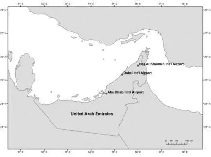
Data from three meteorological stations located in the main international airports of the 147
UAE, where total rainfall is recorded on a daily basis, is used in the present study. Fig. 1 provides 148
the spatial distribution of the meteorological stations. The station of Ras Al Khaimah is located 149
near the north-eastern mountainous region while the Abu Dhabi and Dubai stations are located 150
along the northern coastline. The western region of the country is not represented by any 151
meteorological stations. The three meteorological stations used in the present study were selected 152
based on the length of their records. 153
A list of the rainfall stations with coordinates, measurement periods and annual rainfall 154
data basis statistics is presented in Table 1. Periods of record range from 30 to 37 years. This 155
represents a situation that is common in hydro-climatology. The last years of data are not available 156
9
as data needs first to be homogenized. On average, Abu Dhabi receives the smallest amount of 157
rain (63 mm) and Ras Al Khaimah receives the highest amount (127 mm). Minimum total annual 158
rainfall amounts are around zero for all stations. The variability of annual rainfall time series is 159
high for all stations with values of the coefficient of variation reaching nearly one. All skewness 160
values are positive indicating right skewed distributions. 161
2.2. Rainfall series 162
From the recorded daily data, the total annual rainfall and the annual maximum daily 163
rainfall were computed for each meteorological station. The use of the calendar year (January 1st 164
to December 31st) to compute annual rainfall series would have resulted in splitting the rainy 165
season between two years. In the present study, the hydrological year starting on September 1st 166
and ending on August 31th has been considered instead for the computation of annual rainfall 167
series. 168
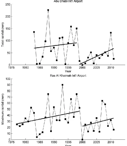
In Ouarda et al. (2014), a change point analysis was performed on the annual rainfall series 169
with a Bayesian multiple change point procedure (Seidou and Ouarda, 2007). A change point 170
around 1999 was detected for all time series. Fig. 2 illustrates examples of rainfall annual series 171
for the total annual rainfall at Abu Dhabi and for the annual maximum rainfall at Ras Al Khaimah. 172
The general pattern shows that there is a positive trend from the beginning of the series to around 173
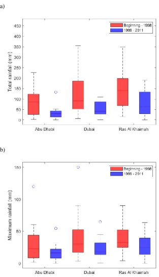
1999, followed by a downward shift and another positive trend until the end. Fig. 3 shows box 174
plots of the samples before and after the change point. In the case of every single time series, we 175
observe an important decrease in the precipitation amount. The shift in the mean, evaluated with 176
the Student’s t-test, was found to be significant for the total annual rainfall but not for the maximum 177
10
annual rainfall. The change in the variance was evaluated with the Levine’s test and revealed a 178
decrease in the variance for the stations of Abu Dhabi and Dubai for the total annual rainfall. 179
2.3 Climate indices 180
Table 2 lists selected climate indices that could potentially be used as covariates in the 181
nonstationary model. A majority of climate indices used in this study was obtained from the Earth 182
System Research Laboratory (ESRL)’s Physical Sciences Division
183
(https://www.esrl.noaa.gov/psd/): the Atlantic Multidecadal Oscillation (AMO), the Arctic 184
Oscillation (AO), the Globally Integrated Angular Momentum (GIAM), the Multivariate ENSO 185
Index (MEI), the North Atlantic Oscillation (NAO), the Oceanic Niño Index (ONI), the Pacific 186
North American Index (PNA), and the Southern Oscillation Index (SOI), the Northern Oscillation 187
Index (NOI), the Pacific Decadal Oscillation (PDO), the Tropical Northern Atlantic Index (TNA), 188
the Tropical Southern Atlantic Index (TSA), and the Western Hemisphere Warm Pool (WHWP). 189
Other climate indices were obtained from the Climate Prediction Center (CPC) at the National 190
Centers for Environmental Prediction (NCEP; https://www.cpc.ncep.noaa.gov/): the East Atlantic 191
Pattern (EA) and the Madden-Julian Oscillation (MJO) pattern. For MJO, the pair of principal 192
component time series, the Real-time Multivariate MJO series 1 and 2 (RMM1 and RMM2), as 193
well as the amplitude of the two MJO principal components (i.e.: RMM12+RMM22 ) are used 194
as climate indices. 195
The Dipole Mode Index (DMI) is used to represent the Indian Ocean Dipole (IOD) 196
phenomenon. Data for DMI was obtained from the Japan Agency for Marine-Earth Science and 197
Technology (http://www.jamstec.go.jp). Data for the Mediterranean Oscillation Index (MOI) was 198
obtained from the Climatic Research Unit at the University of East Anglia 199
11
(https://crudata.uea.ac.uk). The majority of these indices are available on a monthly basis. RMM1, 200
RMM2 and MOI, being available on a daily basis were averaged over each month to obtain 201
monthly series. 202
3. Probability distribution assessment
203
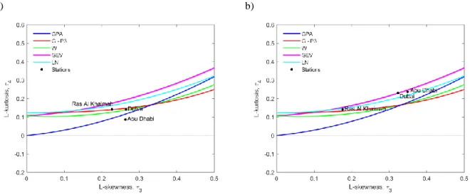
The choice of the distributions to model rainfall variables is justified by the literature and 204
the use of L-moment ratio diagrams. The L-moment ratio diagram is often used to select suitable 205
pdfs to model time series. L-moment ratio diagrams, introduced by Hosking (1990), are commonly 206
used in hydro-climatology (Javelle et al., 2003; Khaliq et al., 2005; Ouarda et al., 2016; Ouarda 207
and Charron, 2019). On the L-moment ratio diagram, the 4th L-moment ratio 4 is represented on 208
the y-axis and the 3th L-moment ratio is represented on the x-axis. For each pdf, all possible 3
209
values of 4 versus are plotted on the diagram. Distributions with only location and/or scale 3 210
parameters plot as a single point, distributions with an additional shape parameter plot as a line 211
and distributions with two or more shape parameters cover a whole area in the L-moment ratio 212
diagram. The moment ratios 4 and are computed for the sample data and are represented by 3 213
points in the moment ratio diagram. The positions of the samples in the diagram are used to infer 214
on the most suitable pdfs. 215
In general, it has been observed that the GEV fits best the annual maximum rainfall data 216
(Adamowski, 1996; Endreny and Pashiardis, 2007; Eslamian and Feizi, 2007; Lee and Maeng, 217
2003; Abolverdi and Khalili, 2010; Cheng & AghaKouchak, 2014). For the total annual rainfalls, 218
the G, GEV, Log-Pearson 3 (LP3) and Pearson 3 (P3) are the most frequently used distributions 219
(Örztürk, 1981; Ben-Gai et al., 2001; Small et al., 2007; Yue and Hashino, 2007; Gonzalez and 220
Valdés, 2008; Hallack-Ageria et al., 2012). Fig. 4 presents the L-moment ratio diagrams with the 221
12
sample moments for each station for the annual maxima and the annual totals. Candidate 222
distributions considered are the Weibull (W), G or P3, Lognormal (LN), Generalized Pareto (GPA) 223
and GEV. For the annual maximum rainfall time series, the GEV is found to be the most suitable 224
pdf, as the samples of the three stations are located near the curve of the GEV. For the total rainfall 225
time series, the G is found to be the most suitable distribution as the samples of the Ras Al Khaimah 226
and Dubai stations are located directly on the curve of the G distribution, while for the sample of 227
the Abu Dhabi station, the G is among the pdfs leading to the best fit. 228
4. Methods
229
4.1. Nonstationary models 230
The cumulative distribution function (cdf) of the GEV is defined by (Coles, 2001): 231
(
)
(
)
1/ exp 1 , 0 ( ; , , ) exp exp , 0 GEV x F x x − − + − = − − − = (1) 232where μ, σ and κ are location, scale and shape parameters respectively, and − / x for 233
0
, − +x for = and 0 − −x / for . In the nonstationary case, the 0 234
distribution parameters are expressed as a function of time dependent covariates: = t and 235
t
= . Given the time dependent covariate Y (which can represent a climate oscillation index), t
236
the following nonstationary models are defined in this study: 237
GEV10 t =a0+a Y1 t and t = , (2a)
238
GEV01 t = and ln(t)= +b0 b Y1 t, (2b)
13
GEV11 t =a0+a Y1 t and ln(t)= +b0 b Y1 t, (2c) 240
GEV20 t =a0+a Y1 t +a Y2 t2 and t = , (2d)
241
GEV21 t =a0+a Y1 t+a Y2 t2 and ln(t)= +b0 b Y1 t. (2e) 242
where a and b are coefficients to estimate. The shape parameter is kept constant ( t = ) as trends 243
in the location and scale parameters are generally more important and is also very difficult to 244
estimate in the presence of small sample sizes (Khaliq et al., 2006). The first index in the model 245
notation in Eqs. 2 refers to the order of the location parameter and the second index refers to the 246
order of the scale parameter. The stationary case model is denoted GEV00 where the location 247
parameter t and the scale parameter t are constant ( t = , t = ). The scale parameter, for 248
models introducing a covariate, is logarithmically transformed to ensure positive values. 249
The cdf of the G is defined by: 250 1 / 0 1 ( ; , ) ( ) x t G F x a b t e dt − − =
(3) 251where β and α are the scale and shape parameters respectively, and 0 and . In the 0 252
nonstationary case, the scale parameter is expressed as a function of time dependent covariates: 253
t
= . Given the time dependent covariate Y (which can represent a climate oscillation index), t
254
the following nonstationary models are defined in this study: 255 G1 ln(t)=a0+a Y1 t, (4a) 256 G2 2 0 1 2 ln(t)=a +a Yt+a Yt (4b) 257
14
where a are coefficients to estimate. The shape parameter is also kept constant ( t = ) for the 258
same reasons as for the GEV. The stationary case model is denoted G0 where the scale parameter 259
is constant (t = ). The scale parameter is logarithmically transformed to ensure positive values. 260
The nonstationary case with two covariates is also considered. Given an additional 261
covariate Z , the distribution parameters depend then on the two covariates t Y and t Z . Different t
262
combinations of these covariates for the distribution parameters are considered. In the present 263
study, we consider a linear and quadratic relation for the location parameter, and a linear relation 264
for the scale parameter. The nonstationary GEV models with two covariates are denoted GEV(iY -265
iZ, jY-jZ) where iY-iZ represents the dependency of the location parameter on the covariates Y and t 266
t
Z , and jY-jZ represents the dependency of the scale parameter on the covariates. For instance, the 267
model GEV(2-1,1-1) indicates that the location parameter has a quadratic relation with the first 268
covariate and a linear relation with the second covariate, and that the scale parameter has a linear 269
relation with both the first and the second covariate (i.e., 2
0 1 2 3
t a a Yt a Yt a Zt
= + + + ,
270
0 1 2
ln(t)= +b b Yt +b Zt). The nonstationary G models with two covariates are denoted G(iY-iZ) 271
where iY-iZ represents the dependency of the scale parameter on the covariates. 272
4.2. Parameter estimation 273
The parameter vectors of these models are estimated with the maximum likelihood 274
method (ML). For a given pdf denoted f, the likelihood function for the sample x ={x ,..., x }1 n is: 275 1 ( ; ) n n t t L f x = =
. (5) 27615
The optimization function fminsearch in MATLAB (MATLAB, 2014) is used to obtain
ˆ, the 277estimator of , that maximizes the likelihood function L . To compare the goodness-of-fit of the n
278
different models, the Akaike information criterion (AIC) is used. It is defined by: 279
AIC= −2ln(Ln) 2+ k (6)
280
where k is the number of parameters of the model. This statistic accounts for the goodness-of-fit 281
of the model and also for the parsimony through the parameter k whose value increases with the 282
model complexity. 283
4.3. Confidence intervals 284
The confidence interval (CI) of an estimated value tells how accurate the estimation is. A 285
commonly used method to compute CIs is the bootstrap. It is a data-based simulation method that 286
allows to make statistical inference on CIs. The method adopted in this study for the computation 287
of the CIs of the estimated quantiles is the parametric bootstrap as described in Efron and 288
Tibshirani (1993). In this method, a parametric estimate Fˆ of the population F with a sample size 289
of n is first obtained. Subsequently, B samples of size n are drawn from the parametric estimate 290
ˆ
F . Then, for each sample, model parameters ˆb, b=1, 2,...,B, are estimated and quantiles 291
1 ˆ
ˆb ( ; b)
q =F− p are evaluated. Finally, the CI around ˆq is computed using the standard deviation 292
of the B estimated quantiles ˆq . b
293
294
5. Results and discussion
16
Prior to carrying out the nonstationary frequency analysis, two covariates representing 296
climate indices are selected to be included in the nonstationary models. A climate index covariate 297
is defined by the average of an index over a season of 3 consecutive months. A season is denoted 298
here by the three first letters of the 3 months included. Seasonal climate index series were built by 299
averaging moving consecutive 3-months windows for the candidate climate indices in Table 2. 300
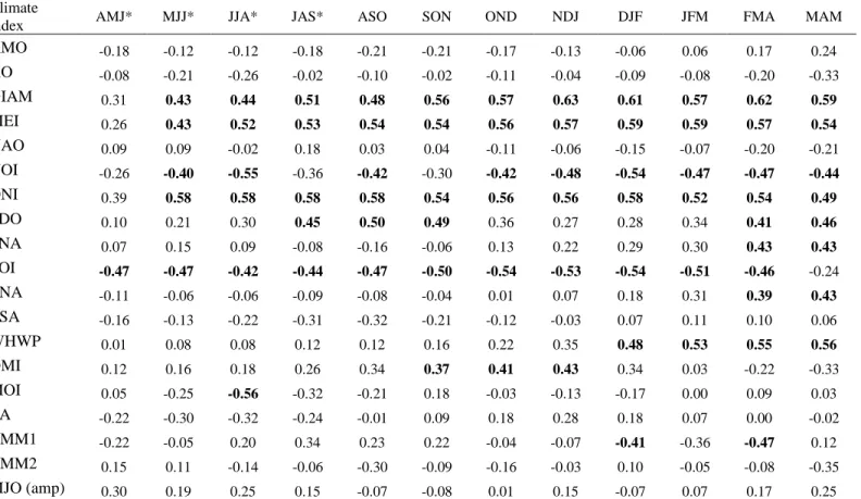
The correlations between the different seasonal climate index series and the annual rainfall series 301
were investigated in order to select the most relevant covariates. Table 3 presents the Pearson 302
correlation coefficients for the total annual rainfall series in Abu Dhabi from the season of April-303
May-June (AMJ*) of the previous hydrological year until March-April-May (MAM) of the same 304
hydrological year than the rainfall events. In Table 3 and in the remainder of the paper, * denotes 305
a season before the hydrological year (September 1st to August 31st) corresponding to the rainfall 306
events. Significant correlations at the 5% level are denoted in bold characters in Table 3. Similar 307
results were obtained for the maximum rainfall and thus are not presented here 308
Covariates are selected based on the significance of the correlations between the rainfall 309
series and the seasonal climate indices. As the interest here is the prediction of rainfalls, covariates 310
were selected during a season preceding the period of December to Mars, which corresponds to 311
the rainy season in the UAE. The climate indices having one or more seasons with a significant 312
correlation with rainfalls are GIAM, MEI, NOI, ONI, PDO, SOI, DMI and MOI. The choice of a 313
covariate within these climate indices was validated with the scatter plots of the rainfall variables 314
versus the covariate. This validation is required after an initial selection as the significance test 315
does not guaranty a causal relationship: The probability of concluding to a significant correlation 316
while it is in fact false is equal to the chosen significance level of 5%. This validation allowed to 317
discard the indices PDO, DMI and MOI. Indeed, even though correlations are high for some 318
17
seasons, the scatter plots for these indices revealed incoherent patterns. For instance, for the PDO 319
index, the correlations are positive but for some cases, the rainfall values are very low even though 320
the corresponding values of this climate index are very high. Retained indices after this validation 321
were GIAM, MEI, NOI, ONI and SOI. All these indices are related to ENSO, proving that this 322
phenomenon is the main oscillation pattern explaining the variance of the precipitation in the 323
region. 324
ONI and NOI for the season JJA*, denoted by ONI(JJA*) and NOI(JJA*), were the 325
selected covariates. ONI(JJA*) was selected because it has one of the highest correlations with the 326
rainfall series. For the selection of the second covariate, intercorrelations between climate indices 327
were checked to avoid the selection of indices that are too similar and reduce redundancy. 328
NOI(JJA*) was selected second because, of all the climate indices retained, NOI has the smallest 329
correlation with ONI (-0.51). Fig. 5 presents the correlations between the total annual rainfall at 330
the three rainfall stations and the three-month moving averages of ONI and NOI. It shows that 331
correlations increase as the index window becomes closer to the rainfall season. Correlations 332
remain significant for several seasons. Finally, correlations decrease to become insignificant 333
towards the end of the rainfall season. The correlations for Dubai are significantly lower than for 334
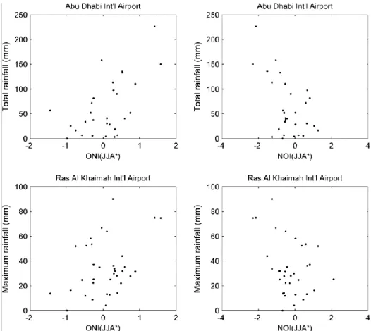
the other stations. Scatter plots of selected covariates with the total annual rainfall at Abu Dhabi 335
and the maximum annual rainfall at Ras Al Khaimah are presented in Fig. 6 as examples. These 336
graphs confirm the choice of the covariates by showing that the rainfall series have coherent 337
relationships with the covariates. 338
The stationary model, the nonstationary model including time as a covariate, and the 339
nonstationary models including each or both selected climate index covariates were fitted to the 340
annual rainfall series. For comparison purposes, the GEV model was also applied to total rainfalls. 341
18
Table 4 presents the values of the AIC criterion obtained for each model. For the nonstationary 342
cases, only the result corresponding to the model leading to the best fit according to AIC is 343
presented. Overall, results indicate that the G model is more appropriate than the GEV for total 344
rainfalls except for Dubai where AIC are lower for the GEV than the G. Results show that adding 345
the time as a covariate reduces in general the goodness-of-fit in comparison to the stationary model. 346
When including a climate index covariate, a better fit than the stationary model is generally 347
obtained. When including ONI and NOI together, the overall best fit is often obtained. The models 348
with time and a climate index as covariates do not generally improve the goodness-of-fit compared 349
to the model with the climate index only. 350
Figs. 7-8 present the quantiles corresponding to the non-exceedance probabilities of p = 351
0.25, 0.5 and 0.75 as a function of the covariate for selected nonstationary models with one 352
covariate. The representation of three quantiles allows to observe changes in both the trend and 353
the variance. Observed data points are also presented in these figures. In each case, the model 354
leading to the best fit is illustrated (see Table 4). The quantiles obtained with the stationary model 355
are also presented in each figure for comparison purposes. 356
Fig. 7a illustrates the quantiles for the total annual rainfall in Abu Dhabi as a function of 357
the time for the nonstationary G model using time as a covariate and fitted to the data over the 358
whole period. The model G1 is retained as the best model. In this case, the variance of the 359
distribution decreases with time due to the negative trend in the scale parameter. It can be observed 360
that quantile values are very small during the last years. They represent bad values for design or 361
management purposes. The nonstationary model with time was also fitted separately to the samples 362
before and after the change point in 1999. The model G1 was retained as the best model for both 363
samples. An example for the total annual rainfall in Abu Dhabi is presented at Fig. 7b. Quantile 364
19
values during the last year are also very low as only the portion of the data with reduced rainfall 365
was used. 366
Fig. 8a presents the quantiles for the total annual rainfall in Abu Dhabi as a function of the 367
covariate ONI(JJA*) and Fig. 8b presents the quantiles for the annual maximum rainfall in Ras Al 368
Khaimah as a function of the covariate NOI(JJA*). The models G1 and GEV20 are respectively 369
retained as the best models. The variance of quantile values shows accordingly a constant increase 370
with ONI in Fig. 8a. A large variation in quantile values as a function of the covariate can be 371
observed in both figures: Quantile values of the median total rainfalls range from about 20 mm to 372
100 mm, and quantile values of the median maximum rainfalls range from about 20 mm to 75 mm. 373
There is a change in the sign of slopes of the quantile curves at the minimum rainfall in the case 374
of maximum rainfalls. This cannot obviously be explained by a climatic phenomenon. This is 375
rather caused by the lack of data for events corresponding to extreme values of the climate indices. 376
The surface plot of the quantiles corresponding to nonexceedance probabilities of p = 0.5 377
and 0.75 for the total and maximum annual rainfall in Abu Dhabi and Ras Al Khaimah as a function 378
of both climate index covariates are presented as examples in Fig. 9. Even though the fit is 379
increased with the two covariates, some problems can be noticed in the graphs of Fig. 9. It was 380
shown in Figs. 6 and 8 that rainfalls generally increase with ONI and decrease with NOI. While 381
these relations are respected for total rainfalls, they are not always respected for maximum rainfalls 382
in Fig. 9. Indeed, maximum rainfall quantiles for p = 0.5 and 0.75 increase with NOI in Abu Dhabi 383
(Fig. 9c), and maximum rainfall quantiles for p = 0.75 decrease with ONI in Ras Al Khaimah (Fig. 384
9d). These problems may indicate that the number of model parameters is too high in the case of 385
the nonstationary GEV model for the size of the data sample and that causes overfitting of the data. 386
This may indicate here that the limits of some models are reached. 387
20
The use of one or the other models presented previously has a strong impact on the 388
estimated rainfall quantiles at a given time. A comparison of the quantile estimates that would be 389
obtained for 2012, the year following the last observed record data, using different models is 390
conducted at the station of Abu Dhabi. Fig. 10 presents, with bar graphs, the predicted quantiles 391
for the probabilities p = [0.5, 0.8, 0.9, 0.95, 0.98, 0.99] corresponding to the classical return periods 392
of 2, 5, 10, 20, 50 and 100 years. Quantiles are defined for nonexceeding probabilities here because 393
under the nonstationary framework, the classical definition of return period is not appropriate (El 394
Adlouni et al., 2007; Salas and Obeysekera, 2014). The following scenarios are considered: the 395
stationary case, the nonstationary case with time as covariate, the nonstationary case with the 396
covariate ONI(JJA*) and the nonstationary case with the two climate index covariates. For total 397
rainfalls, only the G model results are presented. For the stationary model and the nonstationary 398
model with time, the models are fitted to the sample defined by the whole observed period, as well 399
as to the subsample from 1983 to 1998 and to the subsample from 1999 to 2011. These subsamples 400
correspond to the data before and after the change point of 1999. For all the nonstationary models, 401
the quantiles presented in Fig. 10 are those predicted for the year 2012. For the nonstationary case 402
with time, the quantiles based on the model fitted for the period 1983-1998 correspond hence to 403
an extrapolation from 1998 to 2012, and those based on the model fitted for the period 1983-2011, 404
to an extrapolation from 2011 to 2012. For the nonstationary models with climate indices, the 405
values of the covariates ONI(JJA*) and NOI(JJA*) are respectively -0.19 and -0.10. 406
It can be observed in Fig. 10 that there are large differences in the predicted quantiles for 407
the different scenarios. Using only the sample from 1999-2011 results in an underestimation of the 408
quantiles compare to those obtained using the sample for the entire period in either the stationary 409
case or the nonstationary case with time as covariate. This is caused by the fact that observed 410
21
rainfalls were weaker during the last years (See Fig. 7). Using only the sample from 1983-1998 411
with the nonstationary model using time as a covariate results in an overestimation of the quantiles 412
compare to those obtained using the sample for the entire period. This is caused by the 413
extrapolation occurring from 1998 to 2012. As the best fits were obtained with nonstationary 414
models including climate indices, the most realistic scenarios should hence be represented by the 415
models including climate indices as covariates. The values of the climate indices used as covariates 416
for 2012 predict a year of low precipitation. As a result, quantiles obtained with the model with 417
one climate index are lower than those corresponding to the stationary model fitted over the whole 418
period. In fact, the nonstationary model with one climate index predicts quantiles that are among 419
the lowest of all scenarios for both rainfall variables. With two climate indices, the quantiles for 420
total rainfalls compare to those obtained with the model with one climate index. For maximum 421
rainfalls, the quantiles compare to those with the model with one climate index for the lowest 422
probabilities but as the probability increases, the quantiles for the model with two covariates 423
become much higher. For maximum rainfall, quantiles become even larger than the stationary case 424
for p 0.95. This is suspicious as climate indices indicate a year with lower precipitation than 425
usual. This last result indicates potential problems with the GEV model with two covariates when 426
quantiles are extrapolated to extreme probabilities. These problems were already noticed in Fig. 9. 427
The remainder of this section will look at the cause of these behaviors. 428
Previous results showed that the nonstationary models with climate indices provide better 429
fits to the data. However, this is true only for frequencies within the range of those observed during 430
the period of record. In frequency analysis, to estimate quantiles corresponding to more extreme 431
probabilities than those observed, we need to extrapolate in the frequency domain. With 432
nonstationary models, additional extrapolation may occur in the domains of the covariates. 433
22
Nonstationary models introduce also supplementary sources of uncertainties: They require the 434
estimation of a larger number of parameters and the covariates have measurement errors. For short 435
time series, the impacts of these sources of uncertainties on the reliability of the predicted quantiles 436
can be significant. The remainder of this section will focus on the comparison of quantile 437
uncertainty for stationary models and nonstationary models with one or two climate index 438
covariates. Quantile uncertainty is assessed in this study through CIs computed with the parametric 439
bootstrap method presented in section 4.3. 440
Fig. 11 presents graphs of the predicted quantiles with the CIs as a function of the 441
nonexceedence probability. The cases of the total rainfalls for the nonstationary models G1 and 442
GEV21 and the maximum rainfalls for the nonstationary model GEV20 in Ras Al Khaimah are 443
illustrated with the covariate NOI(JJA*) taking the values of -2.25 and 0.5. The selected values of 444
the covariate correspond to scenarios of low and high rainfalls (see Fig. 8). In all cases, the width 445
of the CIs increases rapidly with the probability. When NOI(JJA*)= −2.25, the upper CIs curve 446
for the total rainfalls leads to improbable high rainfall estimations as the probability increases. The 447
G1, a simpler model than GEV21, has an upper CIs curve that is much lower than the one for 448
GEV21. For instance, the width of the CI is accentuated by the negative trend on the scale 449
parameter for model GEV21 which results in a larger variance for extreme negative values of 450
NOI(JJA*). For maximum rainfalls and NOI(JJA*)= −2.25, the width of the CI for the 451
nonstationary model is larger than the width of the CI for the stationary model at the lowest 452
probabilities (approximatively for p 0.95). For NOI(JJA*) = 0.5 and for both rainfall variables, 453
the widths of the CIs for the nonstationary and the stationary models are comparable. In the cases 454
presented, for the lowest probabilities, the nonstationary model leads to quantiles that are 455
significantly different from the stationary model. As the probability increases, the CIs 456
23
corresponding to both models overlap in large parts and each CI eventually includes the predicted 457
quantiles of the other. 458
Fig. 12 presents the quantiles for p = 0.5 as a function of NOI(JJA*) for total and maximum 459
annual rainfalls in Ras Al Khaimah using the models G1 and GEV20 respectively. For some ranges 460
of values of the climate index, the CIs overlap in large part and the CIs of the nonstationary model 461
can encompass completely the CIs of the stationary model. For maximum rainfalls and 462
NOI(JJA*) −1.5, the CIs of both models are totally distinct. The widths of the CIs for the 463
nonstationary model increase as the climate index value becomes more extreme. This is explained 464
by the lack of observed data in the extremes range. 465
Fig. 13 presents similar graphs to Fig. 11 but for the nonstationary model with two 466
covariates. Two cases with real observed covariate values are illustrated: the year 1988, 467
corresponding to high rainfalls (ONI(JJA*)=1.41 and NOI(JJA*)= −2.14) and the year 2001, 468
corresponding to low rainfalls (ONI(JJA*)=-0.58 and NOI(JJA*)=0.19). With two covariates, 469
the widths of the CIs for the nonstationary GEV models are much larger than with one covariate. 470
In most cases, this leads to improbable values for the upper CIs in the highest probabilities 471
(approximatively for p 0.95). Also, for the highest probabilities, the CIs of nonstationary 472
models overlap in a large part or encompass entirely the CIs of stationary models. For the 473
nonstationary G models, the CIs are similar to those obtained with one covariate. This shows that 474
G is more appropriate than GEV for total rainfalls at Ras Al Khaimah: In addition of giving a 475
better fit, G has narrower CIs with two covariates. 476
The previous results show that even if the fit is often better with nonstationary models, the 477
uncertainties on quantile estimates associated to these models can be very important. These 478
24
uncertainties are more important in the extremes range in both the frequency domain and the 479
covariates domains. Because of the importance of these uncertainties, there may be no advantage 480
in using a nonstationary model for certain frequencies or covariate values. When the CIs of the 481
quantiles estimated by the nonstationary model and by the stationary model overlap significantly, 482
the results given by the nonstationary models are judged not sufficiently distinct from those of the 483
stationary model to justify the use of a more complex model. Uncertainties increase significantly 484
with the use of two covariates in the nonstationary model. This is caused by the increased model 485
complexity that often results from the inclusion of an additional covariate and from the 486
measurement errors associated to that covariate. The results of the study demonstrate that 487
nonstationary models should be used with caution. The complexity of nonstationary models should 488
be limited especially with small sample sizes. Extrapolation within the frequency domain should 489
also be limited. 490
6. Conclusions
491
Severe nonstationarities were observed in rainfall time series in the UAE: a change in the 492
rainfall regime in 1999 and the presence of trends. This situation represents a challenge for 493
stationary frequency analysis models. To deals with these issues, nonstationary models introducing 494
covariates in the distribution parameters were used. 495
The nonstationary model including time as a covariate was found to be inefficient given 496
the presence of a change point. Fitting this model separately on the subsamples before and after 497
the change point represent a better solution, but the inconvenient is that the sample size is reduced 498
drastically. Also, a major drawback of using nonstationary models with time as covariate is the 499
increased uncertainty with extrapolation as future trends are not known. On the other hand, 500
25
nonstationary models including a climate index are more promising. In either case, it is important 501
to have a clear understanding of the dynamics and the phenomena involved. These results agree 502
with Agilan and Umamahesh (2017) where the authors have shown that time may not be the best 503
covariate and that it is important to analyze all possible covariates to model nonstationarity. 504
The influence of climate oscillation patterns on the hydro-climatological variables over the 505
region has been well established in many studies (Basha et al., 2015; Niranjan Kumar et al., 2016; 506
Kumar et al., 2017). Seasonal climate index series built from moving windows of average 507
consecutive 3-months were correlated with the annual rainfall series. Oscillation patterns related 508
to ENSO were identified as having a major influence over the region. Based on the correlations of 509
the seasonal climate index series with the annual rainfall series, average ONI and NOI during the 510
months of Jun-Jul-Aug were selected as covariates. The selected covariates were introduced 511
separately and together in the nonstationary models. Significant improvements were obtained with 512
a model including at least one climate index compared to the stationary model, and a model 513
including two climate indices gave in general the overall best fit. 514
The fact that the fit is increased does not guaranty that the predictions are more reliable. 515
With nonstationary models, the complexity is increased because of the additional parameters. The 516
use of two covariates involves even more complex models and the second covariate brings 517
additional measurement errors to the model. To assess the uncertainties, CIs for the predicted 518
quantiles were computed with the parametric bootstrap method. A comparison of the CIs 519
corresponding to the stationary and nonstationary models was conducted. 520
As the probability increases, the CIs of nonstationary models become wider rapidly and 521
can lead to improbable quantile predictions. With two covariates, uncertainties associated to 522
26
predicted quantiles can become considerably large. For moderate probabilities, the CIs of predicted 523
quantiles corresponding to stationary and nonstationary models are often distinct, but for high 524
nonexceedance probabilities, the CIs overlap in large parts. For some ranges of values of the 525
climate index used as covariate, the CIs of both models also overlap considerably, even for low 526
probabilities (for instance 0.5). In these cases, the use of the more complex nonstationary model 527
may not be justified as the predictions of both models are similar. Similar conclusions were also 528
obtained in Ganguli and Coulibaly (2017), where despite the presence of nonstationary signals in 529
short-duration rainfall extremes, statistically indistinguishable differences were obtained between 530
stationary and nonstationary return level estimates. 531
Nonstationary models can still be very useful as they allow to adapt hydro-climatic 532
quantiles to changing conditions. However, they should be used with caution especially with small 533
sample sizes. Indeed, in this case, uncertainties can be very high when quantiles are extrapolated 534
with respect to the return period or the covariate values. 535
Acknowledgment
536
The authors thank the National Sciences and Engineering Research Council of Canada (NSERC) 537
and the Canada Research Chair Program for funding this research. The authors wish to thank the 538
UAE National Centre of Meteorology (NCM) for having supplied the data used in this study. The 539
authors are grateful to the Editor, Dr. Radan Huth, to the Associate Editor, Dr. Enric Aguilar, and 540
to two anonymous reviewers for their comments which helped improve the quality of the 541
manuscript. 542
27
References
543
Abolverdi, J., Khalili, D., 2010. Development of Regional Rainfall Annual Maxima for 544
Southwestern Iran by L-Moments. Water Resources Management 24(11), 2501-2526. 545
Adamowski, K., Alila, Y., Pilon, P.J., 1996. Regional rainfall distribution for Canada. 546
Atmospheric Research 42(1-4), 75-88. 547
Agilan, V., Umamahesh, N.V., 2017. What are the best covariates for developing non-stationary 548
rainfall Intensity-Duration-Frequency relationship? Advances in Water Resources, 101: 549
11-22. 550
Akaike, H., 1973. Information theory and an extension of the maximum likelihood principle. In: 551
Petrov, B.N., Csáki, F. (Ed.), Second International Symposium on Information Theory. 552
Akademinai Kiado, Budapest, Hungary, pp. 267-281. 553
Ashok, K., Saji, N.H., 2007. On the impacts of ENSO and Indian Ocean dipole events on sub-554
regional Indian summer monsoon rainfall. Natural Hazards 42(2), 273-285. 555
Basha, G., Marpu, P.R., Ouarda, T.B.M.J., 2015. Tropospheric temperature climatology and trends 556
observed over the Middle East. Journal of Atmospheric and Solar-Terrestrial Physics, 133: 557
79-86. 558
Ben-Gai, T., Bitan, A., Manes, A., Alpert, P., Rubin, S., 1998. Spatial and Temporal Changes in 559
Rainfall Frequency Distribution Patterns in Israel. Theoretical and Applied Climatology, 560
61(3): 177-190. 561
Chandran, A., Basha, G., Ouarda, T.B.M.J., 2015. Influence of Climate Oscillations on 562
Temperature and Precipitation over the United Arab Emirates. International Journal of 563
Climatology, 36(1), 225-235. 564
28
Cheng, L., AghaKouchak, A., 2014. Nonstationary Precipitation Intensity-Duration-Frequency 565
Curves for Infrastructure Design in a Changing Climate. Scientific Reports, 4: 7093. 566
Coles, S., 2001. An introduction to statistical modeling of extreme values. Springer, London, 208 567
pp. 568
Cullen, H., Kaplan, A., Arkin, P., deMenocal, P., 2002. Impact of the North Atlantic Oscillation 569
on Middle Eastern Climate and Streamflow. Climatic Change 55(3), 315-338. 570
Dezfuli, A., Karamouz, M., Araghinejad, S., 2010. On the relationship of regional meteorological 571
drought with SOI and NAO over southwest Iran. Theoretical and Applied Climatology 572
100(1-2), 57-66. 573
Dimri, A.P., 2013. Relationship between ENSO phases with Northwest India winter precipitation. 574
International Journal of Climatology 33(8), 1917-1923. 575
Efron, B., Tibshirani, R.J., 1993. An Introduction to the Bootstrap. Chapman & Hall/CRC, New 576
York, 456 pp. 577
El Adlouni, S., Ouarda, T.B.J.M., Zhang, X., Roy, R., Bobee, B., 2007. Generalized maximum 578
likelihood estimators for the nonstationary generalized extreme value model. Water 579
Resources Research 43(3), W03410. 580
El Adlouni, S., Ouarda, T.B.M.J., 2009. Joint Bayesian model selection and parameter estimation 581
of the generalized extreme value model with covariates using birth-death Markov chain 582
Monte Carlo. Water Resources Research 45(6), W06403. 583
Endreny, T.A., Pashiardis, S., 2007. The error and bias of supplementing a short, arid climate, 584
rainfall record with regional vs. global frequency analysis. Journal of Hydrology 334(1-2), 585
174-182. 586
29
Eslamian, S.S., Feizi, H., 2007. Maximum Monthly Rainfall Analysis Using L-Moments for an 587
Arid Region in Isfahan Province, Iran. Journal of Applied Meteorology and Climatology 588
46(4), 494-503. 589
FAO, 2008. Irrigation in the Middle East region in figures: AQUASTAT Survey - 2008. water 590
report, 34 pp. 591
Ganguli, P., Coulibaly, P., 2017. Does nonstationarity in rainfall require nonstationary intensity– 592
duration–frequency curves? Hydrology and Earth System Sciences, 21(12): 6461-6483. 593
Ganguli, P., Coulibaly, P., 2019. Assessment of future changes in intensity-duration-frequency 594
curves for Southern Ontario using North American (NA)-CORDEX models with 595
nonstationary methods. Journal of Hydrology: Regional Studies, 22: 100587. 596
Ghasemi, A.R., Khalili, D., 2008. The association between regional and global atmospheric 597
patterns and winter precipitation in Iran. Atmospheric Research 88(2), 116-133. 598
Gonzalez, J., Valdes, J.B., 2008. A regional monthly precipitation simulation model based on an 599
L-moment smoothed statistical regionalization approach. Journal of Hydrology, 348(1-2): 600
27-39. 601
Hallack-Alegria, M., Ramirez-Hernandez, J., Watkins, D.W., 2012. ENSO-conditioned rainfall 602
drought frequency analysis in northwest Baja California, Mexico. International Journal of 603
Climatology 32(6), 831-842. 604
Hosking, J.R.M., 1990. L-Moments: Analysis and estimation of distributions using linear 605
combinations of order statistics. Journal of the Royal Statistical Society. Series B 606
(Methodological) 52(1), 105-124. 607
Hundecha, Y., St-Hilaire, A., Ouarda, T.B.M.J., El Adlouni, S., Gachon, P., 2008. A Nonstationary 608
Extreme Value Analysis for the Assessment of Changes in Extreme Annual Wind Speed 609
30
over the Gulf of St. Lawrence, Canada. Journal of Applied Meteorology and Climatology 610
47(11), 2745-2759. 611
Javelle, P., Ouarda, T.B.M.J., Bobée, B., 2003. Spring flood analysis using the flood-duration– 612
frequency approach: application to the provinces of Quebec and Ontario, Canada. 613
Hydrological Processes, 17(18): 3717-3736. 614
Katz, R.W., Parlange, M.B., Naveau, P., 2002. Statistics of extremes in hydrology. Advances in 615
Water Resources 25(8–12), 1287-1304. 616
Khaliq, M.N., Ouarda, T.B.M.J., Ondo, J.C., Gachon, P., Bobée, B., 2006. Frequency analysis of 617
a sequence of dependent and/or non-stationary hydro-meteorological observations: A 618
review. Journal of Hydrology 329(3–4), 534-552. 619
Khaliq, M.N., St-Hilaire, A., Ouarda, T.B.M.J., Bobée, B., 2005. Frequency analysis and temporal 620
pattern of occurrences of southern Quebec heatwaves. International Journal of 621
Climatology, 25(4): 485-504. 622
Krishnamurthy, V., Goswami, B.N., 2000. Indian monsoon-ENSO relationship on interdecadal 623
timescale. Journal of Climate 13(3), 579-595. 624
Kumar, K.N., Molini, A., Ouarda, T.B.M.J., Rajeevan, M.N., 2017. North Atlantic controls on 625
wintertime warm extremes and aridification trends in the Middle East. Scientific Reports, 626
7(1): 12301. 627
Lee, S.H., Maeng, S.J., 2003. Frequency analysis of extreme rainfall using L-moment. Irrigation 628
and Drainage 52(3), 219-230. 629
Lins, H.F., Cohn, T.A., 2011. Stationarity: Wanted Dead or Alive? JAWRA Journal of the 630
American Water Resources Association 47(3), 475-480. 631
MATLAB, 2014. version 8.3.0 (R2014a). The MathWorks Inc., Natick, Massachusetts. 632
31
Milly, P.C.D., Betancourt, J., Falkenmark, M., Hirsch, R.M., Kundzewicz, Z.W., Lettenmaier, 633
D.P., Stouffer, R.J., 2008. Stationarity Is Dead: Whither Water Management? Science 634
319(5863), 573-574. 635
Naizghi, M.S., Ouarda, T.B.M.J., 2017. Teleconnections and analysis of long-term wind speed 636
variability in the UAE. International Journal of Climatology, 37(1): 230-248. 637
Nazemosadat, M.J., Ghasemi, A.R., 2004. Quantifying the ENSO-Related Shifts in the Intensity 638
and Probability of Drought and Wet Periods in Iran. Journal of Climate 17(20), 4005-4018. 639
Niranjan Kumar, K., Ouarda, T., 2014. Precipitation variability over UAE and global SST 640
teleconnections. Journal of Geophysical Research: Atmospheres 119(17), 10,313-10,322. 641
Niranjan Kumar, K., Ouarda, T.B.M.J., Sandeep, S., Ajayamohan, R.S., 2016. Wintertime 642
precipitation variability over the Arabian Peninsula and its relationship with ENSO in the 643
CAM4 simulations. Climate Dynamics, 47(7-8): 2443-2454. 644
Öztürk, A., 1981. On the Study of a Probability Distribution for Precipitation Totals. Journal of 645
Applied Meteorology, 20(12): 1499-1505. 646
Ouarda, T.B.M.J., Charron, C., 2018. Nonstationary Temperature-Duration-Frequency curves. 647
Scientific Reports, 8(1): 15493. 648
Ouarda, T.B.M.J., Charron, C., 2019. Changes in the distribution of hydro-climatic extremes in a 649
non-stationary framework. Scientific Reports, 9(1): 8104. 650
Ouarda, T.B.M.J., Charron, C., Chebana, F., 2016. Review of criteria for the selection of 651
probability distributions for wind speed data and introduction of the moment and L-652
moment ratio diagram methods, with a case study. Energy Conversion and Management, 653
124: 247-265. 654
32
Ouarda, T.B.M.J., Charron, C., Niranjan Kumar, K., Marpu, P.R., Ghedira, H., Molini, A., Khayal, 655
I., 2014. Evolution of the rainfall regime in the United Arab Emirates. Journal of Hydrology 656
514(0), 258-270. 657
Ouarda, T.B.M.J., El-Adlouni, S., 2011. Bayesian Nonstationary Frequency Analysis of 658
Hydrological Variables. JAWRA Journal of the American Water Resources Association 659
47(3), 496-505. 660
Ouarda, T.B.M.J., Yousef, L.A., Charron, C., 2019. Non-stationary intensity-duration-frequency 661
curves integrating information concerning teleconnections and climate change. 662
International Journal of Climatology 39(4), 2306-2323. 663
Salas, J., Obeysekera, J., 2014. Revisiting the Concepts of Return Period and Risk for 664
Nonstationary Hydrologic Extreme Events. Journal of Hydrologic Engineering 19(3), 554-665
568. 666
Seidou, O., Ouarda, T.B.M.J., 2007. Recursion-based multiple changepoint detection in multiple 667
linear regression and application to river streamflows. Water Resources Research 43(7), 668
W07404. 669
Serinaldi, F., Kilsby, C.G., 2015. Stationarity is undead: uncertainty dominates the distribution of 670
extremes. Advances in Water Resources 77, 17-36. 671
Small, D., Islam, S., 2007. Decadal variability in the frequency of fall precipitation over the United 672
States. Geophysical Research Letters, 34(2), L02404. 673
Strupczewski, W.G., Singh, V.P., Feluch, W., 2001. Non-stationary approach to at-site flood 674
frequency modelling I. Maximum likelihood estimation. Journal of Hydrology 248(1–4), 675
123-142. 676
33
Thiombiano, A.N., El Adlouni, S., St-Hilaire, A., Ouarda, T.B.M.J., El-Jabi, N., 2017. 677
Nonstationary frequency analysis of extreme daily precipitation amounts in Southeastern 678
Canada using a peaks-over-threshold approach. Theoretical and Applied Climatology, 679
129(1-2): 413-426. 680
Thiombiano, A.N., St-Hilaire, A., El Adlouni, S.-E., Ouarda, T.B.M.J., 2018. Nonlinear response 681
of precipitation to climate indices using a non-stationary Poisson-generalized Pareto 682
model: case study of southeastern Canada. International Journal of Climatology, 38(S1): 683
e875-e888. 684
Villarini, G., Smith, J.A., Serinaldi, F., Bales, J., Bates, P.D., Krajewski, W.F., 2009. Flood 685
frequency analysis for nonstationary annual peak records in an urban drainage basin. 686
Advances in Water Resources 32(8), 1255-1266. 687
Wang, X.L., Swail, V.R., 2006. Climate change signal and uncertainty in projections of ocean 688
wave heights. Climate Dynamics 26(2-3), 109-126. 689
Wang, X.L., Trewin, B., Feng, Y., Jones, D., 2013. Historical changes in Australian temperature 690
extremes as inferred from extreme value distribution analysis. Geophysical Research 691
Letters 40(3), 573-578. 692
Yue, S., Hashino, M., 2007. Probability distribution of annual, seasonal and monthly precipitation 693
in Japan. Hydrological Sciences Journal 52(5), 863-877. 694
34
Tables
Table 1. Description of rainfall stations and characteristics of total annual rainfall time series. Minimum, maximum, mean, dimensionless L-moment
ratios of variation (2), skewness (3) and kurtosis (4).
Station name Latitude Longitude Altitude (m)
Period Years Min (mm) Max (mm) Mean (mm) 2 3 4
Abu Dhabi Int’l Airport 24°26' N 54°39' E 27 1982-2011 30 0.0 226 63 0.50 0.26 0.09 Dubai Int’l Airport 25°15' N 55°20' E 8 1975-2011 37 0.3 355 93 0.44 0.26 0.14 Ras Al Khaimah Int’l Airport 25°37' N 55°56' E 31 1976-2011 36 0.0 461 127 0.42 0.22 0.14
35
Table 2. Potential climate indices to be used as covariates in nonstationary models.
Climate index name Symbol
Atlantic Multidecadal Oscillation AMO
Arctic Oscillation AO
Dipole Mode Index (Indian Ocean Dipole) DMI
East Atlantic Pattern EA
Globally Integrated Angular Momentum GIAM
Multivariate ENSO Index MEI
Madden-Julian Oscillation (Amplitude) MJO(amp)
Mediterranean Oscillation Index MOI
North Atlantic Oscillation NAO
Northern Oscillation Index NOI
Oceanic Niño Index ONI
Pacific Decadal Oscillation PDO
Pacific North American Index PNA
Real-time Multivariate MJO series1 RMM1 Real-time Multivariate MJO series2 RMM2
Southern Oscillation Index SOI
Tropical Northern Atlantic Index TNA
Tropical Southern Atlantic Index TSA