Science Arts & Métiers (SAM)
is an open access repository that collects the work of Arts et Métiers Institute of
Technology researchers and makes it freely available over the web where possible.
This is an author-deposited version published in: https://sam.ensam.eu Handle ID: .http://hdl.handle.net/10985/7694
To cite this version :
Julie DIANI, Pierre GILORMINI, Gerry AGBOBADA - Experimental study and numerical simulation of the vertical bounce of a polymer ball over a wide temperature range - Journal of Materials Science - Vol. 49, n°5, p.2154-2163 - 2014
Any correspondence concerning this service should be sent to the repository Administrator : archiveouverte@ensam.eu
Experimental study and numerical simulation of the vertical
bounce of a polymer ball over a wide temperature range
Julie Diani · Pierre Gilormini · Gerry Agbobada
Abstract The dependence to temperature of the
re-bound of a solid polymer ball on a rigid slab is in-vestigated. An acrylate polymer ball is brought to a wide range of temperatures, covering its glass to rub-bery transition, and let fall on a granite slab while the coefficient of restitution, duration of contact, and force history are measured experimentally. The ball fabrica-tion is controlled in the lab, allowing the mechanical characterization of the material by classic dynamic me-chanical analysis (DMA). Finite element simulations of the rebound at various temperatures are run, consider-ing the material as viscoelatic and as satisfyconsider-ing a WLF equation for its time-temperature superposition prop-erty. A comparison between the experiments and the simulations shows the strong link between viscoelastic-ity and time-temperature superposition properties of the material and the bounce characteristics of the ball.
Keywords Polymers · Rebound · Viscoelasticity ·
Thermomechanics
1 Introduction
The vertical bounce of a ball dropped on a flat rigid slab is a classical problem in Solid Mechanics, with ob-vious applications in sports, for instance ([1], [2], [3], among others). For symmetry reasons, this problem is equivalent to the frontal collision of two identical balls with exactly opposite velocities, unless such phenomena
J. Diani· P. Gilormini · G. Agbobada
Laboratoire PIMM, Arts et M´etiers ParisTech, CNRS, 151
Bd de l’Hˆopital, 75013 Paris, France
Tel.: +33-1-44246192 Fax: +33-1-44246382 E-mail: julie.diani@ensam.eu
as acoustic emission are considered (as in [4], for exam-ple), and thus is connected to a wide range of applica-tions (from the collision of fruits [5] up to the stability of planetary rings [6], for instance). A long list of scien-tific papers has followed the celebrated work of Hertz [7] on elastic balls, which took into account more com-plex mechanical behaviors like viscoelasticity ([8] and many others) or viscoplasticity [9]. A plastic behavior was considered essentially in the “dual” problem of the vertical bounce of a rigid ball on a deformable material, especially for the interpretation of the Shore hardness test on metals [10]. Polymers were also considered early in this dual problem ([11], [12], [13]), with attempts to correlate the coefficient of restitution to the damping factor of the viscoelastic material ([14], [15], [16]).
The present paper deals with the bounce of a vis-coelastic solid homogeneous ball, which is simpler in a sense than the hollow (tennis, squash, for instance) or solid but heterogeneous (golf, baseball, etc.) balls used in sports. By contrast, a special effort is put here on a complete control of the ball, which is manufactured in the lab, and on a systematic identification of the mechanical behavior of its constitutive material. More-over, the simple question “Does a ball rebound higher or lower when temperature is increased?” is addressed, and the influence of temperature from the glassy to the rubbery state is investigated. To the authors knowledge, this is the first study of the coefficient of restitution of a polymer ball over such a wide temperature range since the early experimental study of Briggs [17] on golf balls. Jenckel and Klein [11], Calvit [15], Raphael and Arme-niades [16], Robbins and Weitzel [18], among others, covered very wide temperature ranges for the bounce of a rigid ball on polymer blocks instead. By contrast, recent measurements on baseballs ([19], [20]) or squash balls [2], for instance, explored narrow temperature
do-mains only. In addition, finite element simulations are also performed in this study to correlate the experi-mental results to the simulations using the identified mechanical behavior. This numerical technique is pre-ferred here, for better reliability, to more or less simpli-fied models ([13], [8], [6], [21]) of the system.
The remainder of the paper is organized as follows. Section 2 presents how the material was synthesized, its mechanical characterization, how the balls were pro-duced, and the experimental setup used to measure the coefficient of restitution, contact duration, and impact force. Section 3 explains how the finite element simula-tions were run. Finally, Section 4 details the experimen-tal results and discusses the comparison with numerical simulations.
2 Material and methods
2.1 Synthesis of the material and production of the balls
The material is an acrylate network obtained by pho-topolymerization, with a composition given elsewhere [22]. The mix consists of 90% in mol of benzyl methacry-late (BMA) with 10% in mol of 550 g/mol molar weight poly(ethylene glycol) dimethacrylate (PEGDMA) used as crosslinker and 0.5% of 2-dimethoxy-2-phenylaceto-phenone (DMPA) as photoinitiator. Once mixed for 10 minutes at room temperature, the polymer solution was either injected between two glass slides in order to ob-tain rectangular plates of 1.3 mm thickness or injected into hollow spherical glass beads to obtain balls of 25 mm diameter. For polymerization, plates and beads were exposed to 365 nm ultra-violet (UV) light in UV chamber UVP CL-1000 during 50 minutes and 2 hours respectively. Notes that due to the transparent color of the glass and the mix, UV radiation penetrates the balls completely. The DMPA is a poor photoinitiator, which helps preventing early polymerization when preparing the mix, but which also increases the required duration of UV exposure for complete polymerization. In order to assess the complete polymerization of the balls, one ball has been cut into two identical hemispheres reveal-ing a complete solid state.
2.2 Mechanical characterization of the material A complete characterization of the material linear vis-coelasticity and of its time-temperature superposition property were carried out in order to possibly relate these thermomechanical properties of the material with its bounce ability.
(a) 10−2 10−1 100 101 106 107 108 109
Storage modulus (Pa)
Frequency (Hz) 37 °C Decreasing temperature ↑ (b) 10−2 10−1 100 101 0 0.2 0.4 0.6 0.8 1 1.2 1.4 1.6 Damping factor Frequency (Hz) ← Decreasing temperature 37 °C
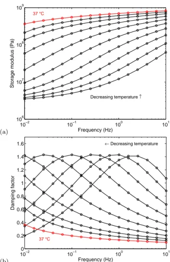
Fig. 1 Temperature dependences of the material storage
modulus (a) and of the damping factor (b) measured dur-ing dynamic torsion frequency sweeps
After identifying the material glass transition tem-perature to 46◦C by differential scanning calorimetry when applying a heating ramp of 10◦C/min, plane sam-ples were submitted to dynamic mechanical analysis in order to characterize the material viscoelasticity. For this purpose, rectangular samples of 40× 12 mm2were cut from the 1.3 mm-thick plates. Theses samples were submitted to dynamic frequency sweep torsion tests on a MCR 502 rheometer from Anton Paar. The applied strain was set to 0.1% for frequencies ranging from 0.01 to 10 Hz. Frequency sweeps were performed at different temperatures, from 37 to 70◦C with 3◦C increments, and three frequency sweep tests were run at each tem-perature. Figure 1 shows the material storage modulus and damping factor dependences to temperature that were obtained.
In order to reach the material viscoelasticity over a wider range of frequencies, the time-temperature su-perposition principle was applied, which provides the material viscoelasticity master curves by mere
horizon-Vertical bounce of a polymer ball 3 (a) 10−3 10−1 101 103 105 106 107 108 109 1010
Storage modulus (Pa)
Frequency (Hz)
Data
Gen. Maxwell fit
(b) 10−3 10−1 101 103 105 0 0.5 1 1.5 Damping factor Frequency (Hz) Data
Gen. Maxwell fit
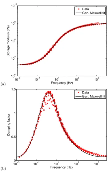
Fig. 2 The acrylate storage modulus (a) and damping factor
(b) master curves at 64◦C, and their fits by a generalized
Maxwell model.
tal shifts of the measured data in Fig. 1. Figure 2 shows the material master curves for the chosen temperature Tref = 64◦C. Figure 2 shows also that this viscoelastic
behavior is reproduced well by a generalized Maxwell model. In order to reach an accurate representation of the material viscoelasticity, 40 relaxation times τi
have been considered, with a fixed ratio of 1.87 between consecutive values. The fitting procedure of Weese [23] was used to obtain the associated set of shear moduli Gi, which applies a Tikhonov nonlinear regularization
that is much more relevant than a mere least squares method. The stiffness of the elastic branch correspond-ing to elasticity at low frequencies was measured to G∞= 2 MPa, and the relaxation times and relaxation moduli are listed in table 1. As a consequence, the re-laxation function in shear writes as
G(t) = G∞+
40
∑
i=1
Gi exp(−t/τi) . (1)
Table 1 Relaxation times and associated shear moduli used
in the generalized Maxwell model.
τi(s) Gi(Pa) 1.259E-08 2.639E+07 2.354E-08 2.256E+07 4.401E-08 1.939E+07 8.230E-08 1.690E+07 1.539E-07 1.505E+07 2.877E-07 1.380E+07 5.380E-07 1.314E+07 1.006E-06 1.310E+07 1.881E-06 1.374E+07 3.517E-06 1.514E+07 6.576E-06 1.739E+07 1.230E-05 2.046E+07 2.299E-05 2.422E+07 4.299E-05 2.822E+07 8.038E-05 3.191E+07 1.503E-04 3.475E+07 2.810E-04 3.648E+07 5.254E-04 3.718E+07 9.824E-04 3.712E+07 1.837E-03 3.632E+07 3.435E-03 3.421E+07 6.422E-03 2.963E+07 1.201E-02 2.226E+07 2.245E-02 1.421E+07 4.198E-02 8.086E+06 7.850E-02 4.416E+06 1.468E-01 2.466E+06 2.744E-01 1.480E+06 5.132E-01 9.806E+05 9.595E-01 6.962E+05 1.794E+00 4.798E+05 3.355E+00 2.875E+05 6.272E+00 1.490E+05 1.173E+01 7.616E+04 2.193E+01 4.540E+04 4.100E+01 3.494E+04 7.667E+01 3.524E+04 1.434E+02 4.427E+04 2.680E+02 6.384E+04 5.012E+02 9.740E+04
Finally, to characterize the material time-tempera-ture superposition, the horizontal shift factors aTref
ap-plied while building the master curves were found to satisfy the Williams-Landel-Ferry (WLF) equation [24]: log10(aTref(T )) =
−C1(T− Tref)
C2+ (T − Tref)
. (2)
Figure 3 shows the shift factor values and their fit by the WLF equation (2) for Tref = 64◦ C, C1 = 17 and
C2= 124◦C.
2.3 Experimental setup
The ball was held by suction with a vacuum pump and was allowed to fall straight from a fixed height of h0=
30 35 40 45 50 55 60 65 70 −1 0 1 2 3 4 5 6 7 Temperature (°C) log 10 (a T ) Shift factors WLF fit
Fig. 3 Time-temperature superposition shift factors and
their fit by the WLF equation.
81.5 cm onto a polished 14× 14 × 10 cm3 granite slab
by turning the pump off. A simple calculation shows that air friction can be neglected during this free fall under gravity, and the velocity of the ball at impact is therefore v0=
√
2gh0≃ 4 m/s.
Two types of measures were carried out. First, sev-eral successive rebounds of the ball on the slab were allowed, and the noise was recorded with a microphone connected to a computer. This gave access to the time between the first two bounces (∆t) by a subsequent simple Matlab [25] treatment of the sound signal, and the upward ball velocity v after the first contact was deduced as v = g∆t/2 by neglecting air friction. This acoustic technique (see for instance Aguiar and Lau-dares [26], among many others), leads to the coefficient of restitution (COR) e = v/v0very simply.
During impact, the ball remains in contact with the slab during a time tc that varies according to the ball
material behavior especially. In order to measure the contact duration of the ball during the first bounce, a thin piezoresistive sensor was stuck on the impacted surface of the slab in a second series of tests. Acoustic measurements confirmed that the COR was not signif-icantly modified by the sensor laying between the ball and the slab during impact, and therefore a possible perturbation induced by the sensor could be neglected. A Flexiforce A401 sensor from Tekscan was integrated in a signal conditioning circuit using an Arduino Uno microcontroller board. In order to increase the record-ing frequency, the output analog signal was saved on a Dso5014A oscilloscope from Agilent Technologies. The Flexiforce sensor provides an easy technical solution to measure the contact duration. It can also give access to the contact force, but a low saturation threshold pre-vents the absolute measure of large forces, and only the
shape of the contact force profile can be studied in such conditions.
The COR and the contact duration were estimated at various temperatures from room temperature to 180◦C. For each temperature, the polymer ball was placed in a thermal chamber for 15 minutes prior to testing. The temperature of the thermal chamber was controlled by a thermocouple run with myPCLab, and at least six rebound tests were performed at each temperature. An additional temperature of 0◦C was also considered for the COR, by cooling the ball in ice before testing.
3 Simulation technique
3.1 Finite element procedure
The Abaqus/Explicit finite element code [27] has been used in this study to perform the simulations of the experimental tests. This software applies an explicit integration scheme to solve highly nonlinear systems with complex contacts under transient loads. It offers a large choice of elements and wide material modeling capabilities. Concerning viscoelasticity, both the gener-alized Maxwell model and the WLF time-temperature superposition relation are available. Moreover, the fi-nite strain extension of the generalized Maxwell model given by Simo [28] is also included, which uses the same relaxation times and shear moduli pairs as those defin-ing the shear modulus master curve for small strains. Therefore, the 40 pairs listed in Table 1 were used. In addition, a reference elastic behavior is required, which was taken as neo-Hookean hyperelastic at high tem-peratures, with a shear modulus of G∞= 2 MPa and a bulk modulus of B = 3.11 GPa. The bulk modulus is assumed independent of temperature and, combined with the shear modulus, the above value leads to a Pois-son’s ratio close to 0.5 in the rubbery state and equal to 0.41 in the glassy state, consequently. The finite el-ement simulations include finite strain.
The ball was meshed as shown in Fig. 4. Axial sym-metry allows one half of the ball section to be mod-eled, and 2278 axisymmetric four-node elements with reduced integration were generated, with smaller ele-ment sizes in the vicinity of the contact area. Since inertia effects are essential in these simulations, a mass density of 1.21 g/cm3 was used, as deduced from the weight and volume measured on the balls. The slab was modeled as a fixed rigid surface with a no-penetration condition imposed. This was allowed by preliminary simulations where the slab was meshed as a 10 cm-high cylinder with a radius of 8 cm (in order to keep axisymmetry and have the same slab volume as in the
Vertical bounce of a polymer ball 5
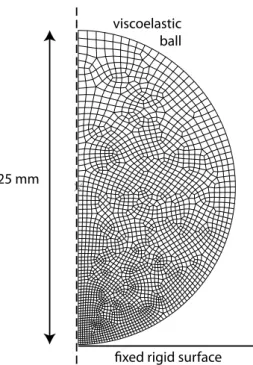
fixed rigid surface viscoelastic
ball
25 mm
Fig. 4 Mesh used in the finite element simulations.
experiments), using standard elastic constants for gran-ite. No difference with the case of a mere rigid surface was found, which is due to a very large contrast of elas-tic properties between the polymer ball and the granite slab (the Young’s modulus is multiplied by about 50 between granite and the glassy polymer, for example), but this equivalence would not apply for a steel ball, for instance. Moreover, no perceptible difference was ob-tained when the ball-slab friction conditions were var-ied, at either low or high temperature, from no friction at all to no slip, which is consistent with contact forces being essentially normal to the interface, and no friction was applied consequently.
At the beginning of the calculations, the ball is lo-cated slightly above the rigid surface, it has a uniform downward velocity of 4 m/s and its temperature also is uniform. Because of the initial position of the ball and because of its low weight (less than 10 grams), the sim-ulations did not show any difference when gravity was taken into account or neglected. Therefore, no gravity loading was applied. The contact duration tc was
de-fined by a non-zero reaction force applied to the fixed rigid surface. The COR e was computed as the ratio be-tween the (upward) velocity of the ball center of mass at the contact end (i.e., when the reaction force returned to zero) and its initial velocity.
3.2 Preliminary simulations
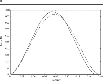
The first preliminary simulation corresponds to the bou-nce of the polymer ball when its elastic glassy behavior is used. In these conditions, the COR should be unity since there is no dissipation in the system considered, except for a low artificial bulk viscosity required for the numerical stability of the integration scheme. As expected, the computed COR is found equal to 1 in-deed. This problem also corresponds to a special case of Hertz’s theory of impact [7], with well-known results ([29], for instance): during contact time, the force ap-plied on the rigid surface is given by
F = 4 3 E√R 1− ν2δ 3 (3) with δ = [ 15 m 16 1− ν2 E√R (v 2 0− ˙δ 2) ]2/5 (4) for a ball of radius R, mass m, Young’s modulus E, Poisson’s ratio ν, with an impact velocity v0. In these
equations, δ denotes the difference between the ball ra-dius and the height of the ball center of mass above the rigid surface. Numerical integration of the differential equation (4) yields a curve shown in Fig. 5, where the result of the finite element simulation also is presented. Although the two curves are close, Hertz’s theory can be observed to give a slightly longer contact duration and a smaller peak force. This theory is recalled to be based on an assumption, which replaces the dynamic problem by a series of static states of equilibrium where the ball is submitted to a different uniform body force at any moment of its contact with the slab. By contrast with this quasi-static approach, the finite element sim-ulation does take the dynamic aspects of the problem into account, a non uniform acceleration is obtained, which gives a non uniform body force, with different results consequently.
In order to confirm the above explanation, a static analysis has also been performed, using the Abaqus/ Standard variant of the code, where a uniform vertical force density was applied instead of an initial veloc-ity. When the pressure profile in the contact area is considered, Fig. 6 shows that a very good agreement is obtained between the finite element simulation and Hertz’s theory. The latter involves a well-known elliptic distribution: p(r) = 3F 2π r 2 c √ 1− ( r rc )2 (5) where rc= ( 3 4 1− ν2 E RF )1/3 (6)
0 100 200 300 400 500 600 700 800 900 1000 0 0.02 0.04 0.06 0.08 0.10 0.12 0.14 0.16 Force (N) Time (ms)
Fig. 5 History of the reaction force on the rigid surface
dur-ing the bounce of the ball in its elastic glassy state. Finite element simulation (solid line) and Hertz’s theory (broken line). 0 20 40 60 80 100 120 140 160 180 0 0.2 0.4 0.6 0.8 1 1.2 1.4 1.6 1.8 Pre ssure (MP a) Radius (mm)
Fig. 6 Pressure profile in the contact area for a static force
of 900 N applied to the ball in its elastic glassy state. Finite element simulation (symbols) and Hertz’s theory (solid line).
denotes the radius of the contact area and F the total applied force. A value of F = 900 N was used to obtain the results of Fig. 6. The discernible difference near the end of the contact area in Fig. 6 can be attributed to the size of the elements used.
As another preliminary test, Abaqus/Explicit has been used to simulate the bounce of the polymer ball in its elastic rubbery state. The ball is now much softer than in the first case considered above (and its behav-ior is nonlinear elastic). Consequently, it has to deform more in order to change its initial kinetic energy into elastic strain energy when the force reaches its maxi-mum (and the first principal logarithmic strain reaches the value of 0.11). As a result, the ball crushes more sig-nificantly on the rigid surface, the maximum radius of the contact area is multiplied by about 3 (close to half the ball radius), and the underlying small deformation assumption in Hertz’s theory is no more valid. This
ex-0 20 40 60 80 100 120 0 0.2 0.4 0.6 0.8 1 1.2 1.4 1.6 Force (N) Time (ms)
Fig. 7 History of the reaction force on the rigid surface
dur-ing the bounce of the ball in its elastic rubbery state. Finite element simulation (solid line) and Hertz’s theory (broken line). The simulation using a Poisson’s ratio of 0.475 is also shown (dotted line).
plains a larger discrepancy with the (finite strain) sim-ulation results in Fig. 7. It may be noted that the areas below the F (t) curves in this figure as well as in Fig. 5 are all equal to 2mv0(twice the initial momentum), as
they should in a non-dissipative impact on a fixed rigid surface. As a result, a factor of about 10 on contact du-ration, which is observed when passing from the glassy (about 0.1 ms) to the rubbery state (about 1 ms), in-duces a factor of about 1/10 on the peak force. As men-tioned previously, the rubbery behavior is very close to incompressible, but Fig. 7 also shows that using a value of ν = 0.475 (keeping the Young’s modulus equal to 6 MPa) does not modify the results significantly. Thus, no bias is induced by the four-node reduced integration elements when quasi-incompressibility is considered in the bounce problem. This can be explained by the ball being quite free to deform, with very few constraints applied on its outer boundary. Unlike Hertz’s theory, which predicts a perfect symmetry of the force history with respect to the force peak, some dissymmetry is evidenced by the finite element results in Fig. 7 (com-pare the curvatures at the beginning and end of con-tact, for instance). This was expected indeed, because the ball keeps vibrating after the contact is left, which differs from its rigid body motion before impact, and therefore the history of the velocity field (and all sub-sequent quantities) must be dissymmetric. This effect is enhanced when the elastic shear modulus of the ball is smaller (compare with Fig. 5), but it does not affect the COR, which remains very close to 1 (0.992, actually). By contrast, a sharp dissymmetry of the force history will be observed when the viscous part of the behavior will be taken into account in the next Section, but this will be due to dissipative effects.
Vertical bounce of a polymer ball 7
4 Results and discussion
4.1 Coefficient of restitution
The experimental measurements of the COR with re-spect to temperature were very reproducible and they are presented in Figure 8. At both low and high tem-peratures, the COR is observed to plateau at its highest value of 0.94. First, it is interesting to notice that the polymer ball bounces as efficiently well at low tempera-ture as at high temperatempera-ture, since this result may seem somewhat counter intuitive according to everyday ex-perience with “superballs”. The latter (like in [1], for instance) are in their rubbery state at room tempera-ture, and one may have the feeling that a glassy ball would bounce less. This is not the case indeed, be-cause the ball is close to elastic at low and at high temperatures as well, and the COR is able to reach equally high values. From 40◦C to 160◦C, the COR is strongly dependent on temperature and, as could be expected, it varies as the viscous component of the be-havior increases, which expresses the delayed mechani-cal response of the material. More precisely, the COR starts decreasing when temperature increases because the relaxation times of the material increase. At higher temperature, the COR increases because the contact duration is increasingly exceeded by relaxation times, and viscous flow has less time to develop. With the vertical axis reversed, the shape of the experimental curve in Fig. 8 may recall the shape of the damping factor plotted as a function of temperature for a fixed frequency, which is somewhat similar to Fig. 2b. This is consistent with the latter curve characterizing energy loss in the material, whereas the COR reflects a fraction of non-dissipated energy, but no direct connection will be attempted here. The experimental results in Fig. 8 follow the same trends as the data of Briggs [17] on golf balls, where a minimal COR was obtained around −40◦C. The right part of the experimental curve in
Fig. 8 is also reminiscent of what is observed on squash balls [2], and warming-up the ball before a game is a common practice that improves the bounce.
The experimental maximum e value is less than 1, which indicates some energy is lost during impacts at low and high temperatures. In the literature, there are many reports of COR values below 1 even though the behavior of the ball could reasonably well be as-sumed to be elastic, and the contributions of acous-tic emission, vibrations, internal friction, slab plasacous-ticity or damage, surface imperfections, adhesion, etc. have been considered. For instance, COR values of 0.95 have been reported in [14] for steel balls impacting steel slabs at moderate velocities. In the present case, it seems
0 50 100 150 200 0 0.1 0.2 0.3 0.4 0.5 0.6 0.7 0.8 0.9 1
Coefficient of restitution (e)
Temperature (°C)
Experimental data Simulations
Fig. 8 Comparison between experimental measures and
sim-ulation estimates of the coefficient of restitution.
reasonable that some viscosity is still present at the extreme temperatures considered, inducing dissipation and a COR less than 1, which is similar to the con-tribution of internal friction invoked in the bounce of metal spheres. Nevertheless, the finite element simula-tions shown in Fig. 8 lead to COR values that are too high at the extreme temperatures considered in the ex-periments, which implies that the dissipation has been underestimated and that the model behavior is very close to perfect elasticity in these conditions. Additional simulations allowed to reject an explanation based on some uncertainty on the impact velocity, since substan-tial variations of the latter were not found to modify the COR significantly. One reason for overestimated COR values can rather be an imperfect rendering of the vis-cous dissipation in extreme cases by the Maxwell model that has been fitted over a limited frequency range and which may ignore a specific effect of high transient strain rates. Another reason can be the limited temper-ature range used in the identification of the behavior (from 30 to 70◦C), and the necessary extrapolation of the WLF equation to temperatures outside this range (from 0 to 180◦C). Finally, it should be mentioned that several (Tref, C1, C2) triplets may fit the data of Fig. 3
equally well, but with a significant impact on the COR predictions.
The shape of the experimental curve in Fig. 8 is nevertheless reproduced well by the finite element sim-ulations, and the minimum value of the COR (0.19 at 84◦C) is estimated quite well (0.22 at 87.5◦C), but some discrepancies remain. In addition to the reasons given above, a possible explanation could be some ex-perimental errors in the temperatures. The temperature within the thermal chamber used to heat the ball was recorded with an accuracy of ±1◦C, but the ball
sur-face may have cooled in the air at ambient temperature during the test duration. Actually, the latter is only a few seconds, which would lead to a temperature gradi-ent located essgradi-entially near the free surface of the ball according to the analytical expressions given in [30]. Such a temperature gradient has been found to have a negligible influence on the COR in additional finite element simulations that we performed. More impor-tantly, the temperatures measured in the thermal cham-ber and in the rheometer have been found to disagree by about 1.8◦C when measured with the same thermo-couple. This lead to a correction that has already been applied in Fig. 8 and cannot explain the differences, consequently. Therefore, the discrepancy between the experimental COR values and the simulations is be-lieved to reflect the limits of the accuracy of the behav-ior provided by standard DMA tests, by the fit with a Maxwell model, and by the extrapolation of the time-temperature superposition.
4.2 Contact duration
The contact duration also is strongly dependent of tem-perature, as shown in Figure 9 where the experimental data obtained with the piezoresistive sensor are pre-sented. Values between 0.13 and 1.2 ms are obtained over the temperature range considered, which confirm that high strain rates develop in the ball during impact. The contact duration appears to depend on the inverse of the material stiffness at impact, and it remains ap-proximately constant below 40◦C and above 120◦C.
Figure 9 presents also the results of the finite ele-ment simulations, which overestimate by about 10% the contact durations at low and high temperatures. This encouraging result is consistent with a possible force threshold below which the sensor does not record con-tact, which induces underestimated experimental val-ues. When temperature increases, the rapid transition between short and long contact durations is also repro-duced quite well.
4.3 Force history during impact
The history of the voltage signal given by the piezore-sistive sensor during impact has been recorded on the oscilloscope. As long as the force is moderate, this sig-nal is proportiosig-nal to the applied force, which allows to measure the actual value of the force with respect to time after calibration has been performed. For in-stance, Fig. 10 shows that the force history recorded at 165◦C is reproduced very well by the finite element simulation. Actually, the latter gives the same results
0 50 100 150 200 0 0.2 0.4 0.6 0.8 1 1.2 1.4 Contact duration (ms) Temperature (°C) Experimental data Simulations
Fig. 9 Comparison between experimental measures of the
contact duration and simulation estimates.
0 0.2 0.4 0.6 0.8 1 1.2 1.4 0 20 40 60 80 100 120 Force (N) Time (ms) Experimental data Simulations 165°C
Fig. 10 Force history during impact at 165◦C.
as the simulation presented in 3.2 where an elastic ball in its rubbery state was considered (Fig. 7), which con-firms that the viscous effects are absent in the model at moderately high temperatures.
Unfortunately, the force becomes so large below 120◦C that a saturation threshold of the sensor is reached. Actually, the points on the sensor surface where the applied pressure is too large saturate, and the total-ized signal of the sensor is affected. As a consequence, the sensor returns the contact area (multiplied by the saturation value) rather than the force in such cases. This happens for instance at room temperature, where the simulations of 3.2 indicated an average pressure of 110 MPa for a glassy ball, i.e. about 100 times larger than in the rubbery case because of a force multiplied by about 10 and a contact area reduced by a factor of about 10. For this reason, the experimental results in Fig. 11 have been scaled vertically to reach the same peak value as the finite element simulation. In these
Vertical bounce of a polymer ball 9 0 0.05 0.1 0.15 0.2 0 100 200 300 400 500 600 700 800 900 1000 Force (N ) Time (ms) Experimental data Simulations 25°C
Fig. 11 Force history during impact at 25◦C. The experi-mental results have been scaled vertically.
conditions, the agreement is acceptable for the whole profile. It may be mentioned that the contact area re-sulting from (6) is proportional to F2/3, and thus would have a convex profile (without the concavities of the theoretical F (t) at the beginning and end of contact) even more similar in shape to the experimental sensor measure, but with a contact time still overestimated. Note finally that the symmetry of the experimental curve in Fig. 11 suggests that the sensor has no hys-teresis, even though it saturates.
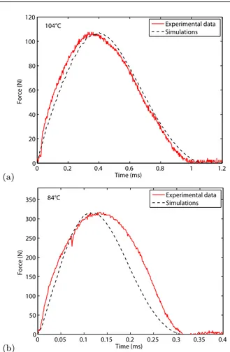
The normalization procedure of the experimental re-sults has also been applied in Fig. 12, where two exam-ples of force histories in the intermediate range of tem-perature is presented, i.e. when viscous dissipation is significant according to Fig. 8. Accordingly, the force vs. time profiles are now clearly unsymmetric. The trend in common with Fig. 10 and Fig. 11 is a decreasing peak force when temperature increases, i.e. the trend opposite to contact duration. Although the force peak is comparable with Fig. 10, some sensor saturation was present at 104◦C (Fig. 12a) because of a smaller contact area, but the agreement with the finite element results is still good when the force normalization is applied. By contrast, the simulated force history at 84◦C (Fig. 12b) differs more significantly from the sensor signal, even though the latter has been adjusted vertically to fit the force peak. A first reason to explain the difference is a strong sensor saturation due to a large pressure, which distorts the experimental force profile. It should also be noted that the temperature of 84◦C corresponds to the smallest experimental coefficient of restitution, and therefore to a maximum viscous dissipation. The dis-crepancy may thus also be due to the approximations and limitations involved in the model used to describe the viscoelastic behavior of the material and in its iden-tification. (a) 0 0.2 0.4 0.6 0.8 1 1.2 0 20 40 60 80 100 120 Force (N ) Time (ms) 104°C Experimental data Simulations (b) 0 0.05 0.1 0.15 0.2 0.25 0.3 0.35 0.4 0 50 100 150 200 250 300 350 Force (N ) Time (ms) Experimental data Simulations 84°C
Fig. 12 Force history during impact at 104◦C (a) and 84◦C (b). The experimental results have been scaled vertically.
5 Conclusion
The effect of temperature on the vertical rebound of a polymer ball falling on a rigid slab has been shown experimentally to be substantial when a wide enough temperature range is considered. This allows to answer the question asked in the Introduction: the coefficient of restitution decreases when temperature increases if the ball is at low temperature, but the opposite trend ap-plies if the ball is above a transition temperature. The contact duration and force history also have been mea-sured, the former increases with temperature, whereas the contrary applies to the peak force.
The fabrication of the acrylate ball in the lab al-lowed a thorough mechanical characterization of the material by dynamic mechanical analysis which, com-bining a generalized Maxwell model and the WLF equa-tion for time-temperature superposiequa-tion, allowed in turn the finite element simulation of the rebounds without ad hoc adjustment. The simulations agreed globally well with the experiments. The trends were predicted correctly, which has shown the strong link between the viscoelastic and time-temperature superposition
prop-erties of the material and the main characteristics of the bounce of a polymer ball.
Nevertheless, some discrepancies remain. Besides ex-perimental difficulties like temperature control or piezo-resistive sensor saturation, this study has shown that re-bound testing enhances the effect of some uncertainties and extrapolations in the description of a temperature-dependent viscoelastic behavior. Moreover, it suggests that some features of the viscoelastic deformation of polymers at high transient strain rates may still be im-properly implemented in simple models of the mechan-ical behavior.
Acknowledgements The authors are grateful to several
col-leagues from PIMM laboratory: J. L´edion for lending his
ther-mal chamber, M. Schneider for making his digital oscilloscope available, and F. Coste for his advice on signal acquisition. Moreover, M. Brieu from LML is acknowledged for giving ac-cess to his mechanical testing machine for sensor calibration.
References
1. Cross R (1999) The bounce of a ball, Am. J. Phys. 67:222-227
2. Lewis GJ, Arnold JC, Griffiths IW (2011) The dynamic behavior of squash balls, Am. J. Phys. 79:291-296
3. Collins F, Brabazon D, Moran K (2011) Viscoelastic im-pact characterisation of solid sports balls used in the Irish sport of hurling, Sports Engng 14:15-25
4. Akay A, Hodgson TH (1978) Acoustic radiation from the elastic impact of a sphere with a slab, Appl. Acous. 11:285-304
5. Dintwa E, Van Zeebroeck M, Ramon H, Tijskens E (2008) Finite element analysis of the dynamic collision of apple fruit, Postharvest Biol. Technol. 49:260-276
6. Hertzsch JM, Spahn F, Brilliantov V (1995) On low-velocity collisions of viscoelastic particles, J. Phys. II France, 5:1725-1738
7. Hertz H (1881) Ueber di Ber¨uhrung fester elastischer
K¨orper, J. reine angw. Math. 92:156-171
8. Kuwabara G, Kono K (1987) Restitution coefficient in a collision between two spheres, Jap. J. Appl. Phys. 26:1230-1233
9. Ismail KA, Stronge WJ (2008) Impact of viscoplastic bod-ies: dissipation and restitution, J. Appl. Mech. 75:061011.1-061011.5
10. Tabor D (1948) A simple theory of static and dynamic hardness, Proc. R. Soc. Lond. A 192:247-274
11. Jenckel E, Klein E (1952) Die Bestimmung von
Re-laxationszeiten aus der R¨uckprallelastizit¨at, Z. Naturf. A
7:619-630
12. Tillett JPA (1954) A study of the impact of spheres on plates, Proc. Phys. Soc. B 67:677-688
13. Hunter SC (1960) The Hertz problem for a rigid spherical indenter and a viscoelastic half-space, J. Mech. Phys. Solids 8:219-234
14. Lifshitz JM, Kolsky H (1964) Some experiments on anelastic rebound, J. Mech. Phys. Solids 12:35-43
15. Calvit HH (1967) Experiments on rebound of steel balls from blocks of polymers, J. Mech. Phys. Solids 15:141-150
16. Raphael T, Armeniades CD (1967) Correlation of re-bound tester and torsion pendulum data on polymer sam-ples, Polym. Engng Sci. 7:21-24
17. Briggs LJ (1945) Methods for Measuring the Coefficient of Restitution and the Spin of a Ball, Research Paper RP1624, National Bureau of Standards
18. Robbins RF, Weitzel DH (1969) An automated resilience
apparatus for polymer studies from−196 to +180◦C, Rev.
Scient. Inst. 40:1014-1017
19. Drane PJ, Sherwood JA (2004) Characterization of the effect of temperature on baseball COR performance, The Engineering of Sports 5, M. Hubbard et al. Eds, vol. 2, 59-65
20. Nathan AM, Smith LV, Faber WL,Russell DA (2011) Corked bats, juiced balls, and humidors: the physics and cheating in baseball, Am. J. Phys. 79:575-580
21. Nagurka M, Huang S (2006) A mass-spring-damper model of a bouncing ball, Int. J. Engng Ed. 22:393-401 22. Safranski D, Gall K (2008) Effect of chemical structure
and crosslinking density on the thermo-mechanical proper-ties and toughness of (meth)acrylate shape memory poly-mer networks, Polypoly-mer 49:4446-4555
23. Weese J (1993) A regularization method for nonlinear ill-posed problems, Comput. Phys. Commun. 77:429-440 24. Williams ML, Landel RF, Ferry JD (1955) The
temper-ature dependence of relaxation mechanisms in amorphous polymers and other glass-forming liquids. J. Amer. Chem. Soc. 77:3701-3707
25. Matlab (2011), The MathWorks Inc., Natick MA, USA 26. Aguiar CE, Laudares F (2003) Listening to the
coeffi-cient of restitution and the gravitational acceleration of a bouncing ball, Am. J. Phys 71:499-501
27. Abaqus (2010) Dassault Systems Simulia Corp., Provi-dence RI, USA
28. Simo JC (1987), On a fully three-dimensional finite-strain viscoelastic damage model: formulation and computational aspects, Comput. Meth. Appl. Mech. Engng 60:153-173 29. Johnson KL (1985) Contact Mechanics, 351-355,
Cam-bridge University Press
30. Carslaw HS, Jaeger HS (1959) Conduction of Heat in Solids, 2nd Ed., 233-234, Clarendon Press