Science Arts & Métiers (SAM)
is an open access repository that collects the work of Arts et Métiers Institute of Technology researchers and makes it freely available over the web where possible.
This is an author-deposited version published in: https://sam.ensam.eu
Handle ID: .http://hdl.handle.net/10985/9492
To cite this version :
Anouar BELAHCEN, Paavo RASILO, Thu Trang NGUYEN, Stéphane CLÉNET - Uncertainty propagation of iron loss from characterization measurements to computation of electrical
machines - COMPEL - The international journal for computation and mathematics in electrical and electronic engineering - Vol. 34, n°3, p.624-636 - 2015
Any correspondence concerning this service should be sent to the repository Administrator : archiveouverte@ensam.eu
Uncertainty Propagation of Iron Loss from Characterization Measurements to Computation of Electrical Machines
Abstract— This paper presents the uncertainty propagation of iron losses from the material
characterization measurements to the computed losses in an induction machine. The iron losses are modelled with an analytical loss model applied locally in finite element simulation. The uncertainty is taken into account by the decomposition into Polynomial Chaos Expansion, i.e., the spectral approach. The results of the simulations show that uncertainties in the measured losses propagate in different ways and to different parts of the machine depending on the measurement frequency and the nature of losses, i.e., hysteresis, eddy current or excess losses. The computations also show that the measurement uncertainties at low frequencies have negligible effect on the accuracy of computed losses whereas those at the supply frequency and higher ones affect very much this accuracy. It is also shown that the most important loss components are those related to the classical eddy current and alternating hysteresis losses especially in the tooth tips of the stator and rotor. The results suggest that more attention should be paid to the measurement and characterization of these sensitive components.
1. Introduction
Electrical machines consume about 40% of the electrical energy produced in the European Union (SEC 2009). The design and simulation of electrical machines and electromechanical energy conversion devices is nowadays exclusively carried out through finite element (FE) based numerical models. These models can be two- or three-dimensional with different approaches in the formulations and the implementations. The accuracy of the numerical simulations of electrical machines has increased in the last decades through better material models and the coupling of the magnetic field and the circuit equations of the windings of the machine. However, this accuracy depends strongly on the parameters of the material models and the manufacturing processes of both the materials and the machine. The computation of the resistive losses is nowadays very accurate and the only problems related to these losses reside in the effect of circulating current in parallel wires of the random windings (Hämäläinen et al. 2013), skin effect in form windings (Islam and Arkkio 2009), and the interbar currents in the case of cage induction machine (Dorrell et al. 2009). On the other hand, the iron losses, which account for up to half of the total losses, are still a subject of extensive investigations and the accuracy of the computed iron losses varies heavily from one author to the other.
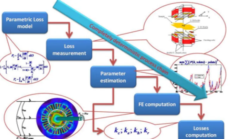
Conventionally, the process of iron loss characterization and computation has a waterfall structure as shown in Figure 1. The whole process starts with some more or less complex model of losses in the electrical steel. The model is usually an analytical one where the losses are computed based on some model parameters and the waveform of the magnetic flux density in the sample (Belahcen and Arkkio 2008, Fratila et al. 2013) but some more advanced models, e.g. magnetodynamic vector hysteresis models (Dlala et al. 2010, Handgruber et al. 2013), are also used. In all cases, the model parameters are estimated from measurements made on electrical steel sheet samples. These measurements could be either standard ones like the Epstein frame or non-standard ones like the Rotational Single Sheet Tester (RSST). Once the model parameters are estimated through some fitting strategy, they are used in conjunction with the numerical simulation of the electrical machine, where the flux density distribution is computed, the iron loss model is applied locally and then the losses are integrated over the volume of the machine core. Such a process is completely deterministic and thus it does not account for the variability introduced by the manufacturing process of both the material and the machine. Indeed, the properties of the same material grade vary within a certain range due to the stochastic nature of the manufacturing process. Further, the punching of iron sheets and the shrink fitting of the iron core as well as the welding deteriorate the material properties in a more or less stochastic way (Krings 2014).
The above uncertainties of the manufacturing processes make the iron loss parameters exhibit stochastic behaviour. So far, the numerical models used in the optimization of electrical machines have typically not accounted for these uncertainties. Since the computed optimal design can be within a narrow region of the design space, even a small deviation from the model parameters will result in a large amount of machines with very inefficient operation (Kim et al. 2010), as schematically illustrated in Figure 2. A better solution of the problem would take the uncertainties into account and fall in a flat local minimum with very little variability of the machine performances, thus ensuring regular quality of the production line.
Fig. 1. Illustration of the deterministic waterfall process for iron loss characterization and computation. The equations and other similar texts are only illustrative; they are reported in details at the corresponding sections of the paper.
Fig. 2. Illustration of the effect of uncertainties on the result of optimization. A sharp global minimum might turn out to be a worst design than a flat local minimum when the uncertainties in the model parameters are taken into account.
In this paper we study the uncertainty propagation of iron losses from the characterization measurements of iron sheets up to the loss computations in induction machines. Two different approaches are taken. In the first one the variability is assumed to be in the loss parameters and in the second one the variability is assumed to be in the measured quantities from which the loss parameters are estimated. In both approaches a stochastic global sensitivity analysis is carried out by assuming uniform probability distributions of the quantities. We show that the uncertainties propagate through the model almost linearly but the distribution of losses in different parts of the machine as well as the segregation of losses depend strongly on the nature of uncertainties. Measurement uncertainties in low frequencies do not affect very much the computed losses whereas uncertainties in the measurements at high frequencies or under rotating fields propagate to either the tooth tips or yoke of the machine.
In Section 2 we present the measurement setup used to characterize the material all together with the measured results. In Section 3 we present the 2D finite element model used to simulate the induction machine under investigations along with the iron loss model. Section 4 explains the stochastic approach used in this work, and Section 5 presents the obtained results and discusses them. At the end a conclusion is given, where the consequences of the presented investigations are summarized and suggestions are given on how the research in this field should be advanced.
2. Method of iron loss characterization
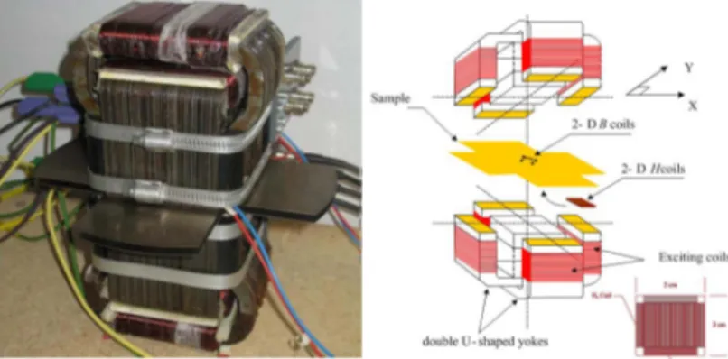
The characterization of electrical steel sheet in this work is carried out on the RSST shown in Figure 3 (Belkasim 2008). The device consists of two vertical U-shaped magnetizing iron cores and the corresponding windings. The windings are supplied by a computer-controlled two-phase power amplifier to produce the desired magnetic flux density in the measuring area of the sample. The field-metric measurement method is used to pick up the magnetic flux density B and the magnetic field strength H vectors. For this purpose two orthogonal B-coils and two calibrated H-coils are utilized as shown in Figure 3. The frequency and the shape of the magnetic flux density are set by the user and controlled by a LabView-based program in the laboratory computer. In our measurements we used frequencies from 10 to 1000 Hz with alternating and rotating flux densities of different amplitudes from 0.2 T up to 1.8 T, in total 250 measurements, each measurement consisting of not less than 3000 samples of the B and H waveforms. The power loss density in W/kg was then computed from the measured B and H as 0 1 T m p d T H B (1)
where is the mass density of the electrical steel sheet (7600 kg/m3) and T is the period of
magnetization.
The measurements will be used later in the paper to estimate the loss model parameters and carry out the sensitivity analysis as to determine how the uncertainty in these measurements will propagate to the computed losses in an induction machine.
Fig. 3. The Rotational Single Sheet Tester used to characterize the electrical steel sheet. Actual device (left) and illustrated parts and instrumentation (right). The supply and control system are not shown.
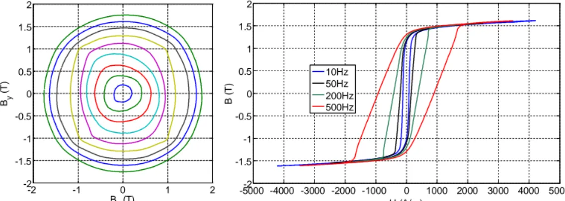
Fig. 4. Examples of measured flux density locus in case of rotating magnetization at 10 Hz and different amplitudes (left) and hysteresis loops for alternating magnetization at 1.6 T and different frequencies (right).
3. Iron loss model and FE simulation
The computation of the iron losses in the software is carried out through an analytical model, where the losses are segregated into four components, i.e. Pc classical eddy current, Pha alternating, and Phr rotational hysteresis, and Pe excess losses according to (Belahcen and Arkkio 2008) and reported here as follows: 2 c c P k d t B (2) ha a P k d t B B (3) 2 1 1 (1 ) s hr r s B P k d t b B B B B (4) 3 2 e e P k d t B (5)
where kc, ka, kr,ke, and b are constant model parameters, Bs is the technical saturation flux density, and is the angular direction of the magnetic flux density vector.
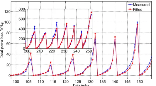
Fitting of the loss model parameters is shown in Figure 5. The x-axis in the figure is an arbitrary number associated with each measurement point. It is seen that the measured and computed losses agree with each other at most of the points. However, at some points the measured and computed losses do not agree very well. This is most likely caused by the fact that the measurements were made in both rolling and transverse directions and the loss parameters for the two directions are not the same. Especially, in case of rotational magnetization, the loss parameters are, in a way, an average of those in rolling and transverse directions.
-2 -1 0 1 2 -2 -1.5 -1 -0.5 0 0.5 1 1.5 2 Bx (T) By (T ) -5000 -4000 -3000 -2000 -1000-2 0 1000 2000 3000 4000 5000 -1.5 -1 -0.5 0 0.5 1 1.5 2 H (A/m) B (T ) 10Hz 50Hz 200Hz 500Hz
Fig. 5. Measured and fitted power loss density for different rotating and alternating magnetization at different amplitudes and frequencies of the magnetic flux density. The alternating losses were measured in both rolling and transverse directions. A noticeable difference between the directions can be seen as well as its effect on the rotational magnetization case. The x-axis represents the experiment number only.
The simulations of the induction machine under investigation are carried out with an in-house, 2D FE software package. The software is based on the A- formulation and it incorporates the coupling between the field and the circuit equations of the windings of the machine. The permeability of the iron core is modelled as a single-valued nonlinear function of the magnetic flux density, and the Newton-Raphson iteration procedure is used to solve the nonlinear problem. The software performs time-harmonic and transient analysis with both current and voltage supply. In the transient case, the Crank-Nicolson time integration scheme is applied. The parameters of the studied machine are given in Table I.
In the FE model, the losses are computed for each element of the mesh from the time-dependent flux density vector and then summed up for each region of the machine separately. The machine is divided into six regions namely the stator yoke, teeth and tooth tips and the rotor yoke, teeth and tooth tips. The flux density distribution in the cross section of the induction machines at the last time step of the simulation is shown in Figure 6, and the computed losses in different parts of the machine and at different loads are given in Table II. The increase of the total iron losses with loading as reported in (Dlala et al. 2012) can be seen as well as the increase of the losses in the stator teeth and tooth tips. Such a result confirms the validity of the deterministic loss model. In the next section the stochastic approach will be explained and its results presented.
Table I. Parameters of the simulated induction machine.
Parameter Value
Rated voltage 380 V
Slip 2.0 %
Rated current 69 A
Rated power 37 kW
Number of pole pairs 2
Outer diameter of the stator core 310 mm
Inner diameter of the stator core 200 mm
100 105 110 115 120 125 130 135 140 145 150 0 20 40 60 80 100 120 Data index T o ta l p o w er lo ss , W /k g Measured Fitted 200 210 220 230 240 250 0 200 400 600 800
Number of stator slots 48
Outer diameter of the rotor core 198.4 mm
Number of rotor slots 40
Fig. 6. Geometry of the simulated induction machine altogether with the flux density distribution at the last time step.
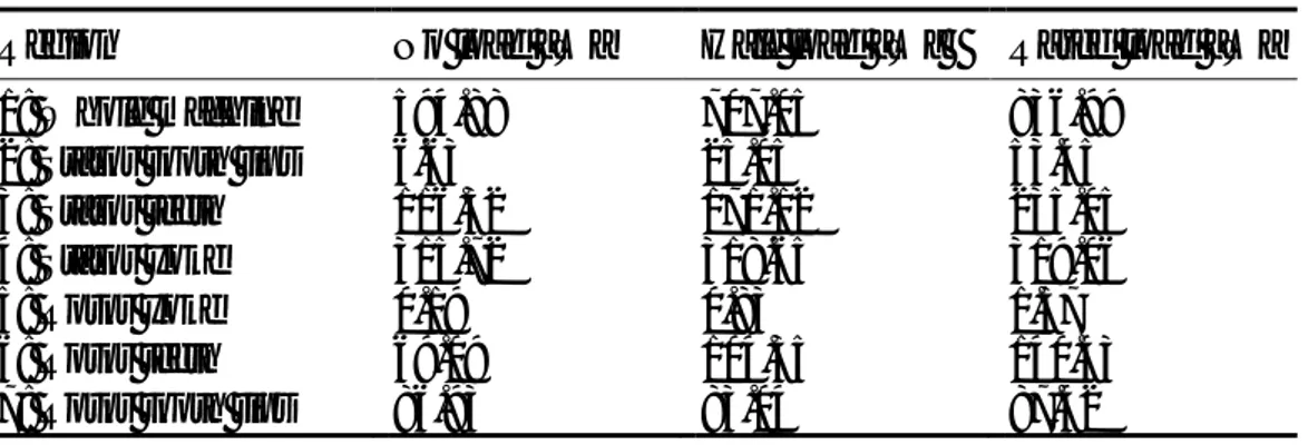
Table II. Computed losses at different regions of the induction machine at different loads.
Region No load [W] Half load [W] Rated load [W]
1: Whole machine 594.88 707.05 836.99
2: Stator tooth tips 6.63 25.05 53.45
3: Stator teeth 116.32 171.12 235.05
4: Stator yoke 315.72 318.65 319.06
5: Rotor yoke 0.19 0.83 1.57
6: Rotor teeth 69.09 104.35 140.43
7: Rotor tooth tips 86.93 83.04 87.42
4. Stochastic approach
To investigate the effect of the measurement uncertainties on the computed losses, we followed two approaches. In the first approach, the loss parameters are supposed to be uncertain and are modelled by uniform random variables, whereas in the second approach the uncertainties are supposed to be due to the measurements and uniform random noises are added to the measured values. In both cases, 10% variation of the quantities is taken as uncertainty range. The first approach thus describes the propagation of uncertainties from the parameters of the model to the computed losses through the FE simulation and loss model, whereas the second approach describes this propagation from measurements to computations as described in (Ramarotafika et al. 2012). The uncertainty itself is quantified using the Sobol indices (Sobol 1993) and the stochastic sensitivity analysis. For this purpose we write the loss parameters or the measured losses as a vector of probability distributions
( )q
X and compute the loss probability distribution as
0 12... 1 1 1 1 ( ( )) ( ( )) ( ( ), ( )) ... ( ( ),...., ( )) M M M i i ij i j M M i i j j i X X X X X Y X Y f f f (6)
where Y stands for the vector of losses in different regions of the machine at different loads, Xi are either the loss coefficient in the first approach or the random noise added to the measurements in the second approach and fi the multidimensional polynomial expansions to be calculated in accordance
( ( ( ))) ( ( )) i i i Var f X S Var Y (7)
where Var stands for the variance of the quantity in question.
5. Results and discussion
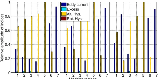
As discussed above, the loss model parameters were first assumed to have a uniform distribution around the deterministic values estimated from the measurements made on the RSST. Meanwhile the induction machine has been simulated with the FE software at no load, half load and full load and the normalized losses at different regions of the machine have been calculated and stored in a separate file. The global sensitivity analysis with the spectral approach has been implemented as a post processing routine in Matlab, where the inputs are the normalized losses and the variability of each of the loss parameters. The outputs of the routine are the first order Sobol indices corresponding to each parameter of the loss model. These indices are shown in Figure 7. Here it can be seen that throughout the machine and independently of the load, the most significant parameters are the ones related to the classical eddy current and the alternating hysteresis losses. The parameter related to the rotational losses has almost no significance. The significance of the eddy current loss parameter increases with the loading in the whole machine and especially in the stator tooth tips.
Fig. 7. Sobol indices for different regions of the machine (1: whole machine, 2: St tooth tips, 3: St teeth, 4: St yoke, 5: Rt yoke, 6: Rt teeth, 7: Rt tooth tips). The left histogram is for no-load case the middle one for half-load and the right for the full load case. The colours describe the variability in the different loss coefficients.Note that the in some regions the columns corresponding to the alternating and rotating hysteresis are hardly seen as their effects are non-significant as discussed in the text.
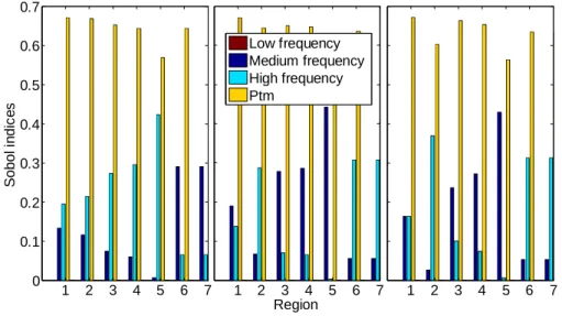
In the second approach, we introduced the uncertainty in the measurements before the estimation of the parameters of the loss model. Here, besides the uncertainty on the measured losses (Ptm in Fig. 8)
according to (1), we subdivided the measurements into three different bunches consisting of the measurements of the magnetic flux densities at low, medium and high frequencies. We here assume also a uniform distribution of uncertainty in the measured losses as computed from the magnetic field strength and the magnetic flux density as well as on the three other bunches as they are depending on the magnetic flux density only. This approach, thus assumes that the uncertainty is on one hand in the measured field strength H and magnetic flux density B as well as in the relative angle between the measurement sensors, and on the other hand the uncertainty is in the measurement of the flux density B. A similar post processing routine implementing the spectral approach is used in this section too but the inputs of this routine are now the measured losses and the three sets of quantities derived from the measured magnetic flux densities altogether with the normalized losses computed by the FE analysis. The Sobol indices for this computation are given in Figure 8. Here one can see clearly that the magnetic flux densities at low frequencies (10 – 30 Hz) have virtually no effect on the computed
1 2 3 4 5 6 7 Machine regions Eddy current Excess Alt. Hys. Rot. Hys. 1 2 3 4 5 6 7 0 0.2 0.4 0.6 0.8 1 R e la ti v e a m p li tu d e o f in d ic e s 1 2 3 4 5 6 7
losses in the induction machine independently of the loading or the region under investigation. This result although it seems to be obvious is not really expected as the loss parameters are not computed based on any harmonic analysis.
The most significant set is the one coming from the measured losses, which are computed based on the magnetic field strengths and the magnetic flux densities. This result was expected as these are the quantities against which the loss model is identified. The importance of the next set related to the medium frequencies (50 – 200 Hz) increases when the load of the machine is different but does not increase anymore from half load to full load. Such a result is emphasised in regions 3-5, i.e. the stator and rotor yokes as well as the stator tooth. The significance of the high frequency components(500 – 1000 Hz) is seen in regions 6 and 7, i.e. the rotor teeth and tooth tips and as the loading increases. Such a result should be compared with the results from Figure 7, where it was shown that at these regions the eddy current losses are the most significant.
As a summary of this study, it could be said that the global accuracy of the iron loss model depends on the accuracy of measurements made at the supply frequency of the machine and higher ones, and that the most significant accuracy of the loss components is the one related to the eddy current and alternating hysteresis losses. Further, measurements at lower frequency than the supply frequency of the machine do not have any effect on the accuracy of loss computation.
Fig. 8. Sobol indices for different regions of the machine (1: whole machine, 2: St tooth tips, 3: St teeth, 4: St yoke, 5: Rt yoke, 6: Rt teeth, 7: Rt tooth tips). The left histogram is for no-load case the middle one for half-load and the right for the full load case. The colours describe the variability in the measured losses at different frequency ranges. Note that the column corresponding to the low frequency is hardly seen as its effects are not significant as discussed in the text.
6. Conclusion and future developments
The above conclusion about the significance of loss components and measurement frequencies are based on assumed probability distributions of the related components. For a better correlation with the real life devices, these probability distributions should be acquired through repetitive measurements of the same grade of the material but from different material lots. This is the only method to obtain realistic data about the variability in the material itself. Further, the effect of manufacturing process variability need real process input that could be retrieved from measurements on constructed machines if the manufacturing series are large enough to allow for statistical analysis. Last but not least, the higher order Sobol indices should be computed for the different stochastic variable in order to quantify their combined effects.
1 2 3 4 5 6 7 0 0.1 0.2 0.3 0.4 0.5 0.6 0.7 S o b o l in d ic e s 1 2 3 4 5 6 7 Region Low frequency Medium frequency High frequency Ptm 1 2 3 4 5 6 7
References
A. Arkkio, 1987, Analysis of induction motors based on the numerical solution of the magnetic field
and circuit equations, Doctoral dissertation, Helsinki University of Technology, Espoo, Finland.
A. Belahcen, A. Arkkio, 2008, “Comprehensive Dynamic Loss Model of Electrical Steel Applied to FE Simulation of Electrical Machines,” IEEE Trans. Magn. , vol. 44, no. 6, pp. 886-889.
M. Belkasim, 2008, Identification of loss models from measurements of the magnetic properties of electrical steel sheets, M.Sc. thesis, TKK Dept. of electrical engineering, Finland, 2008. Available at: http://lib.tkk.fi/Dipl/2008/urn012787.pdf
E. Dlala, A. Belahcen, K. Fonteyn, M. Belkasim, 2010, “Improving loss properties of the Mayergoyz vector hysteresis model,” IEEE Trans. Magn., vol. 46, no. 3, pp. 918-924.
D.G. Dorrell, P.J. Holik, P. Lombard, H.-J. Thougaard, F. Jensen, 2009, “A Multisliced Finite-Element Model for Induction Machines Incorporating Interbar Current,” IEEE Trans. Ind. App., vol.45, no.1, pp.131-141.
M. Fratila, A. Benabou and A. Tounzi, 2013, “Improved iron loss calculation for non-centered minor loops,” COMPEL: The International Journal for Computation and Mathematics in Electrical and Electronic Engineering, vol. 32, no. 4, pp. 1358-1365
H. Hamalainen, J. Pyrhonen, J. Nerg, 2013, “AC Resistance Factor in One-Layer Form-Wound Winding Used in Rotating Electrical Machines,” IEEE Trans. Magn. , vol. 49, no. 6, pp. 2967-2973. P. Handgruber, A. Stermecki, O. Biro, A. Belahcen, E. Dlala, 2013, “Three-Dimensional Eddy-Current Analysis in Steel Laminations of Electrical Machines as a Contribution for Improved Iron Loss Modeling,” IEEE Trans. Ind. App., vol.49, no.5, pp. 2044-2052.
M. J. Islam, A. Arkkio, 2009, “Effects of pulse-width-modulated supply voltage on eddy currents in the form-wound stator winding of a cage induction motor,” IET Electric Power Applications, vol. 3, no. 1, pp. 50-58.
N-K Kim, D-H Kim, D-W Kim, H-G Kim; D.A. Lowther, J.K. Sykulski, 2010, “Robust Optimization Utilizing the Second-Order Design Sensitivity Information,” IEEE Trans. Magn., Vol.46, No.8, pp. 3117-3120.
A. Krings, 2014, Iron Losses in Electrical Machines-Influence of Material Properties, Manufacturing
Processes, and Inverter Operation, Doctoral thesis, KTH School of Electrical Engineering,
Stockholm, Sweden, 177 p.
R. Ramarotafika, A. Benabou, S. Clenet, 2012, “Stochastic Modeling of Soft Magnetic Properties of Electrical Steels: Application to Stators of Electrical Machines,” IEEE Trans Magn. , vol. 48, no. 10, pp. 2573-2584.
SEC(2009) 1014 final, Commission staff working document, Accompanying document to the proposal for a commission regulation implementing directive 2005/32/ec with regard to motors, Summary impact assessment, Brussels, 22.7.2009.
I.M. Sobol, 1993, “Sensitivity Estimates for Nonlinear Mathematical Models,” Mathematical Modelling and Computational Experiments, vol. 1, pp 407-414.