Science Arts & Métiers (SAM)
is an open access repository that collects the work of Arts et Métiers Institute of Technology researchers and makes it freely available over the web where possible.
This is an author-deposited version published in: https://sam.ensam.eu
Handle ID: .http://hdl.handle.net/10985/17961
To cite this version :
Taoufik QORAI, Chuanyue LI, Ko OUE, François GRUSON, Frédéric COLAS, Xavier GUILLAUD - Direct AC Voltage Control for Grid-Forming Inverters - Journal of Power Electronics p.13 - 2019
Any correspondence concerning this service should be sent to the repository Administrator : [email protected]
Vol.:(0123456789)
1 3
ORIGINAL ARTICLE
Direct AC voltage control for grid‑forming inverters
Taoufik Qoria1 · Chuanyue Li1 · Ko Oue1 · Francois Gruson1 · Frederic Colas1 · Xavier Guillaud1 Received: 13 April 2019 / Revised: 22 July 2019 / Accepted: 12 August 2019
© The Korean Institute of Power Electronics 2019 Abstract
Grid-forming inverters usually use inner cascaded controllers to regulate output AC voltage and converter output current. However, at the power transmission system level where the power inverter bandwidth is limited, i.e., low switching frequency, it is difficult to tune controller parameters to achieve the desired performances because of control loop interactions. In this paper, a direct AC voltage control-based state-feedback control is applied. Its control gains are tuned using a linear quadratic regulator. In addition, a sensitivity analysis is proposed to choose the right cost factors that allow the system to achieve the imposed specifications. Conventionally, a system based on direct AC voltage control has no restriction on the inverter cur-rent. Hence, in this paper, a threshold virtual impedance has been added to the state-feedback control in order to protect the inverter against overcurrent. The robustness of the proposed control is assessed for different short-circuit ratios using small-signal stability analysis. Then, it is checked in different grid topologies using time domain simulations. An experimental test bench is developed in order to validate the proposed control.
Keywords Power transmission system · 2-Level voltage source inverter · Grid-forming control · State-feedback control · Small-signal stability analysis · Current limitation · Transient power coupling
1 Introduction
An ever-increasing number of renewable energy production systems and HVDC systems are being connected to the grid. This has led to an increase in power electronic devices in the power system. Nowadays, synchronous generators (SGs) are dominating the electrical grid, establishing a stable volt-age and frequency that allow for voltvolt-age source inverters (VSIs) to be synchronized at the point of common coupling (PCC) through a phase-locked loop (PLL) and injecting the power to the grid. These inverters are characterized as “grid-following” VSIs and behave as current sources. However, since the installation of these generating units is rapidly increasing, some synchronous areas might occasionally operate without synchronous machines. In such conditions, and since the power inverter-based grid-following concept is not able to form an instantaneous AC voltage [1], the system may lose synchronism, which can lead to unstable
operation. As a result, electrical power can no longer be provided to loads. Therefore, the present operation mode is dramatically changed, while the grid stability still has to be ensured with the same level of reliability as today, or better. To operate autonomously, the control law should be changed. Power inverters need to change from following the grid to leading the grid behavior [1–4]. This capability is known as the “grid-forming” concept, where power inverters are able to generate an AC voltage with a given amplitude and frequency at the PCC.
The inner control is usually ensured by cascaded PI con-trollers. Conventionally, PI controllers are independently tuned by considering a sufficient frequency separation between the control loops, i.e., to avoid interactions, where the current loop dynamics is limited by the inverter band-width. This control structure is favored due to the ease of its implementation and its design. In addition to the con-ventional PI controllers, many other control strategies have been used for grid-following and grid-forming. Predictive control [5], table-based control [6], fuzzy logic control [7], repetitive control [8] and neural network-based control [9] have been proposed for grid-following. For the grid-form-ing concept, some control techniques have been proposed such as sliding mode control for the inner current loop and
* Taoufik Qoria [email protected]
1 Univ. Lille, Centrale Lille, Arts et Metiers ParisTech,
HEI, EA2697, L2EP, Laboratoire d’Electrotechnique de Puissance, 59000 Lille, France
a mixed H2∕H∞ for the AC voltage loop [10]. This
con-trol technique aims to design a robust concon-troller to achieve high performances. However, this technique is complex and requires very high computations. In a recent paper, a frac-tional order controller was proposed for grid-forming invert-ers. It was motivated by its flexibility and its high number of degrees of freedom. Among the control strategies proposed for grid-forming inverters, a few studies have discussed the control design in high-power applications [10, 11] where the switching frequency is lower than 5 kHz. Such condition can result in a slow dynamics [11], restrained stability regions and interactions between control loops, which can lead to an unstable system [12]. Therefore, controller parameter tuning in such conditions is still a challenge.
This paper focuses mainly on VSI grid-forming control tuning for high-power application. It is an extension of the work done in [13] and refers to work done in [11]. In the latter, the authors proposed an algorithm that deduces the cascaded PI controller gains based on eigenvalues location. This method improves the system stability. However, the AC voltage response time is still very large; the system is poorly damped and presents a strong transient coupling between the AC voltage and the active power. Moreover, because of the control loop interactions, it is not possible to achieve desired performances. In this paper, the cascaded control structure is replaced with a direct AC voltage regulator based on state-feedback control, which aims to enhance the AC voltage dynamics and allows for achieving desired performances. Employing a system state-space model, the controller gains are designed based on a linear quadratic regulator (LQR). Usually, LQR cost factors are designed manually [13–15]. However, in this paper, a sensitivity analysis is proposed to choose the LQR cost factors. The controller tuning considers both the AC voltage response time and the transient coupling between the AC voltage and the active power. To assess the robustness of the developed control, an AC grid impedance variation is performed.
The major disadvantage of the direct AC voltage control is its inability to handle the VSI output current, which can lead to system damage in case of overcurrent. Indeed, when compared to synchronous machines that can support up to seven times over its rated current, power inverters can only cope with few percent of overcurrent (20–40%). Therefore, inverters have to be protected against extreme events such as short circuits and other events that can induce a small overcurrent such as phase shift, connection of large loads and tripping of a line protect power converter against over-current [16]. Since the proposed control does not have a servo-current control to limit current transients, a parallel threshold virtual impedance (TVI) [2] is adopted and com-bined with the proposed AC voltage control.
Several test cases are performed based on single and multi-inverter systems. The aim is to check the effectiveness
of the developed control to operate stably under normal and abnormal scenarios that can occur in power transmission systems. Finally, the developed control is validated on an experimental test bench.
This paper is organized as follows. Section II presents the system modeling of a 2-level VSI and recalls the conven-tional structure of inner cascaded PI controllers. In Section III, the proposed direct AC voltage control embedding the current limitation algorithm is presented, analyzed and vali-dated using time domain simulations. Section IV performs some tests in different grid topologies in order to demon-strate the effectiveness of the developed control. In Section V, the developed control is validated in an experimental test bench. Finally, some conclusions are drawn in Section VI.
2 Grid‑forming based on the conventional
cascaded control structure
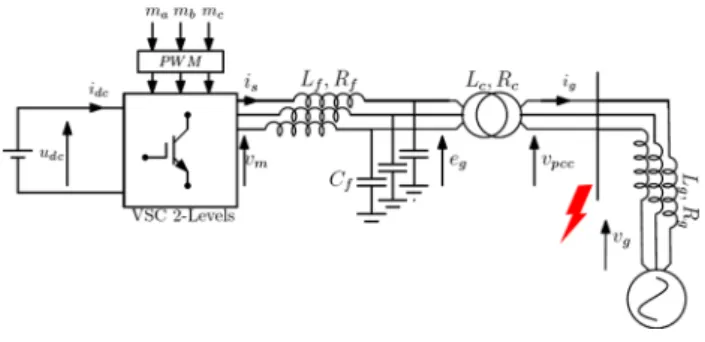
2.1 System modelingThe system illustrated in Fig. 1 consists of a three-phase 2-level voltage source inverter represented by a switching model. It is supplied by a DC voltage source that is assumed to be a DC storage and/or primary source, i.e., PV, wind tur-bine, etc., and connected to an AC system through an LfCfLc
filter. The AC system is model by an equivalent AC voltage source in series with its equivalent impedance Zg= Rg+ jXj ,
i.e., the AC system is assumed to be a stiff symmetrical AC system.
Following the notations in Fig. 1, the state variables are the VSI output current is through the filter inductor Lf , the
AC voltage eg across the filter capacitor Cf , and the grid
current ig through the equivalent transformer inductance Lc.
For the system analysis, only the average modeling of the system is used. Then, a switching model is used to validate the proposed control by time domain simulations.
The state variables are represented in the d − q frame using a Park transform. The following is a state-space model of a three-phase system at the device level:
Fig. 1 Power electronic converter connected to an AC system via an LCL filter
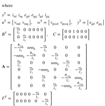
where
All of the variables are expressed in per unit. The vectors x , u and w are the system state variables, the system inputs supposed to be the modulated voltage vmdq and the system disturbances supposed to be the AC voltage at the PCC vpccdq. The output y is the AC voltage egdq . In addition, 𝜔b and 𝜔
are the base value for the angular frequency in rad∕s and the nominal frequency in per unit, respectively.
2.2 Conventional control structure
Figure 2 presents the grid-forming cascaded control struc-ture. It consists of an inner cascaded AC voltage and a VSI output current control represented in the synchronous refer-ence frame (SRF). The inner voltage control is ensured by two proportional–integral (PI) controllers considering the (1) { ̇ x= [A]x + [B]u + [F]w y= [C]x (2) xT= isd isq egd egq igd igq uT =�vmd vmq�, wT=�vpccd vpccq�, yT =�egd egq� BT = �𝜔b Lf 0 0 0 0 0 0 𝜔b Lf 0 0 0 0 � , C= � 0 0 1 0 0 0 0 0 0 1 0 0 � 𝐀 = ⎡ ⎢ ⎢ ⎢ ⎢ ⎢ ⎢ ⎢ ⎢ ⎢ ⎣ −Rf 𝜔b Lf 𝜔𝜔b − 𝜔b Lf 0 0 0 −𝜔𝜔b − Rf 𝜔b Lf 0 −𝜔b Lf 0 0 𝜔b Cf 0 0 𝜔𝜔b − 𝜔b Cf 0 0 𝜔b Cf −𝜔𝜔b 0 0 − 𝜔b Cf 0 0 𝜔b Lc 0 − Rc 𝜔b Lc 𝜔𝜔b 0 0 0 𝜔b Lc −𝜔𝜔b − Rc 𝜔b Lc ⎤ ⎥ ⎥ ⎥ ⎥ ⎥ ⎥ ⎥ ⎥ ⎥ ⎦ FT= � 0 0 0 0 −𝜔b Lc 0 0 0 0 0 0 −𝜔b Lc �
feedforward decoupling Cf𝜔egdq and compensation igdq . The inner current control is also is ensured by two propor-tional–integral (PI) controllers considering the feedforward decoupling Lf𝜔isdq and compensation egdq.
kpv and kiv are the proportional gain and integral gain for the AC voltage control, respectively. Meanwhile, kpc and kic
are the proportional gain and integral gain for the VSI cur-rent control, respectively.
The current control loop generates the modulated voltage to the linearization stage that delivers the modulation signals to the switching stage of the inverter. The control angle 𝜃VSC
and the AC voltage reference e∗
gdq are provided by the
pri-mary control based on the droop control P − 𝜔 and Eg− Q
droop.
The primary control is expressed by the following equations:
where 𝜔VSC , mp and nq are the VSI output frequency, active
droop gain and reactive droop gain, respectively. The low-pass filter in the reactive power droop aims to filter the measurement noises. Meanwhile, the low-pass filter used in the active power droop aims to simultaneously filter the measurement noises and emulate the inertia effect of the synchronous machine [17–19].
Conventionally, the controllers in the cascaded structure are independently tuned by setting a lower response time for the inner current loop, i.e., fastest eigenvalues, which is limited by the first-order transfer function approximating the PWM effect [20] in (5), and a higher response time for the outer loops:
(3) 𝜔VSC− 𝜔set= mp𝜔c 𝜔c+ s(pmes− p ∗) (4) e∗gd− Eset= nq [ qmes ( 1 1+ TQs ) − q∗ ]
where fs𝜔 denotes the switching frequency.
The conventional controller tuning for grid-forming inverter-based cascaded structure shows its effectiveness in terms of ensuring stable operation in the standalone mode, but suffers from instability issues in the grid-connected mode following the analysis in [12, 21]. The instability is mainly caused by the inner current control loop [12]. Thus, the next section presents an alternative control structure based on direct AC voltage control.
3 Direct AC voltage control for grid‑forming
inverters
The direct AC voltage control depicted in Fig. 3 consists of a state-feedback controller and an integral compensator.
K and Ki are the pole placement gains ( 2 × 6 ) and the servo-controller gains (2 × 2) , respectively.
The vector 𝜁 denotes the error derivative between the AC voltage references r and the measured output voltage egdq:
The augmented controlled system matrices can be writ-ten as:
where I denotes the identity matrix. The control gains ̄K =[−KKi
]
are tuned based on linear quadratic control. This provides a control gains matrix based on the minimization of the performance index J in (11):
(5) TPWM= 1 1+ 1 2fs𝜔 s (6) r=[e∗ gd e ∗ gq ]T (7) ̇𝜁 = r − y = r − Cx (8) [ ̇ x ̇𝜁 ] = A 0 −C 0 [ x 𝜁 ] + [ B 0 ] u+ [ 0 I ] r+ [ F 0 ] w (9) y=[C 0][x 𝜁 ]T (10) u= −Kx + Ki𝜁= − [ K −Ki ] [x 𝜁 ]T
where Q and R are positive-definite/positive-semidefinite Hermitian matrices. The first term on the right side of (11)
̄
xTQ̄x is related to the convergence speed of each state
vari-able. The second term uTRu accounts for the expenditure of
the control signals energy.
The optimum gain matrix ̄K is expressed as follows: where P is the solution of the RICCATI function [22]:
The existence of the matrix P implies the system stability. One of the most common (initial) LQR tuning approaches is to consider all of the cost factors equally [23], i.e., Rk= [I]2×2 and Qi= [I]8×8 . This initial parametrization is used to check the system stability and the AC voltage dynamics. Thus, the choice of cost factors is improved thanks to the parametric sensitivity analysis.
3.1 LQR cost factors design
Based on the parameters listed in Table 1 and the ini-tial parameterization of the cost factors Qi= [I]8×8 and
Rk= [I]2×2 , the eigenvalues of the linear system (see appen-dix) listed in Table 2 have a negative real part, which results in stable system operation.
In order to check the inner AC voltage loop dynamics, time domain simulations are shown in Fig. 4. These simula-tions are performed in MATLAB/SimPowerSystem.
(11) J= ∞ ∫ 0 (̄xTQ̄x+ uTRu)dt (12) ̄ K= R−1B̄TP (13) ̄ ATP+ P ̄A + Q − P ̄BR−1B̄TP= 0
Fig. 3 Block diagram of direct AC voltage control
Table 1 System parameters Parameter Value
Pn 1 GW cos 𝜑 0.95 fn 50 Hz Uac 320 kV Rf, Rc 0.005 p.u Lf, Lc 0.15 p.u Cf 0.066 p.u mp 2% Eset 1 p.u Rg 0.005 p.u Lg 0.05 p.u 𝜔c 31.4 rad/s nq 1e−4 p.u fsw 4 kHz
A voltage step of Δe∗
gdq= 0.03pu is applied at t = 1s in both the d− axis and the q− axis.
The obtained results in Fig. 4 show that both the d − q AC voltage components have a slow first-order response, where Trd−axis = 8.1s and Trq−axis = 6s:
where Tr denotes the response time.
The dynamics of the d-axis AC voltage corresponds exactly to the eigenvalue 𝜆10= −0.36445 + 0i:
The q-axis AC voltage dynamics corresponds exactly to the eigenvalue 𝜆11= −0.49623 + 0i:
In order to improve the AC voltage dynamics, it is impor-tant to find the link between the eigenvalues and the system parameters to target the parameters that impact the AC volt-age dynamics. This link is found using a parametric sensi-tivities tool. The parameter sensisensi-tivities of 𝜆i are defined
as the derivative of eigenvalues with respect to the control (14) Tr 5% = 3∕ √( ℜ2+ ℑ2)= 8.1682s. (15) Tr 5% = 3∕ √( ℜ2+ ℑ2)= 6.0456s.
parameters. Thus, these sensitivities can identify the param-eters that strongly impact specified eigenvalues (i.e., 𝜆10−11 )
[24].
Since the aim is to improve the dynamic of the states xi , only the cost factors Qi are tuned. The sensitivity sℜ−ℑ
of the eigenvalues 𝜆i with respect to the parameter Qi is
expressed by the following expressions:
The real and imaginary parts of the sensitivities are associated with the derivatives of the pole location along the ℜ and ℑ axes, respectively.
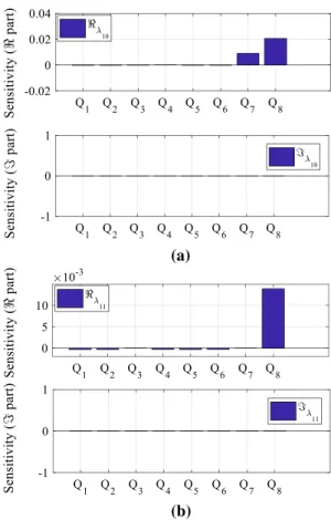
Figure 5 shows that only Q7−8 have a large impact on the
eigenvalues 𝜆10−11 . Thus, the AC voltage dynamics can be
improved by tuning these cost factors.
The choice of the cost factors is made according to the following specifications:
• Ensuring a reasonable voltage response and a low over-shoot. (16) sℜ= 𝜕ℜ𝜆i 𝜕Qi , sℑ= 𝜕ℑ𝜆i 𝜕Qi .
Table 2 System eigenvalues Eigenvalue Location
𝜆1−2 −758.65 ± 5507.4i 𝜆3−4 −758.92 ± 4879.2i 𝜆5−6 −12.356 ± 311.23i 𝜆7−8 −14.652 ± 39.50i 𝜆9 −31.416 + 0i 𝜆10 −0.36445 + 0i 𝜆11 −0.49623 + 0i
Fig. 4 AC voltage dynamics for Q = [I]8×8 and R = [I]2×2
(a)
(b)
Fig. 5 Parameter sensitivity analysis, eigenvalues corresponding to the AC voltage: a d-axis; b q-axis
• Ensuring a transient power decoupling. This criterion is not considered in most voltage controller tuning methods [10–12, 21].
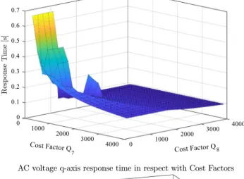
A variation of the cost factors Q7−8 results in a
varia-tion of 𝜆10−11 . This, in turn, leads to a modification of the
AC voltage response time as depicted in Fig. 6, where it is ascertainable that the response time of the AC voltage loop decreases when Q7−8 increase. This demonstrates the
capability and flexibility of the proposed method to achieve different response times for the AC voltage in comparison with cascaded PI controllers structures [11, 12].
The time domain simulations in Fig. 7 show the impact of the AC voltage dynamics on the active power. It can be seen that the increase in the AC voltage rise time (rise time = response time for the first-order response) results in a high transient coupling with the active power. Therefore, it is important to choose the cost factors in such a way as to ensure both a low-power transient coupling and a reasonable AC voltage convergence dynamics.
From Figs. 6 and 7, the response time of the AC voltage is set to Tr5% = 200ms . This specification is reasonable for power transmission systems applications. This specification corresponds to Q7= 1500 and Q8= 100.
Based on the defined response time and cost factors, the control parameters and the new system eigenvalues are listed in Tables 3 and 4, respectively.
Compared to Table 2, Table 5 shows that only 𝜆10−11 ,
which correspond to the voltage loop dynamics, are modi-fied while the rest of eigenvalues have not been impacted.
3.2 Comparison with conventional methods
In order to show the relevance of the proposed method, a comparison with the method in [11] has been performed.
Fig. 6 Impact of the cost factors Q7−8 on the AC voltage response
time
Fig. 7 AC voltage change and its impact on the active power Table 3 Controller parameters
Parameter Value K [0.72 0 1.02 0 −0.73 0 0 0.7197 1.2e− 3 1.014 −0.0004 −0.72 ] KI [−38.62 −2.88 0.744 −9.9722 ]
Table 4 System eigenvalues Eigenvalue Location
𝜆1−2 −758.32 ± 5511i 𝜆3−4 −758.94 ± 4882i 𝜆5−6 −12.385 ± 312.97i 𝜆7−8 −14.864 ± 21.38i 𝜆9 −31.41 + 0i 𝜆10 −13.982 + 0i 𝜆11 −5.3441 + 0i
The same analysis done in this paper has been applied to the system parameters used in [11]. These results are listed in the following table and used only for comparison.
Based on the system parameters in Table 5, the controller gains deduced from the developed method in this paper are listed in Table 6.
The performed test case in Fig. 8 consists of applying a voltage change of − 10% at t = 1 s.
When compared to the conventional method, the obtained results in Fig. 8 clearly show the improvements brought by
the proposed method, where the developed method has a smooth AC voltage change without overshoot. Moreover, the specified AC voltage dynamics result in a negligible cou-pling with the active power.
3.3 Control robustness against grid impedance variation
The robustness of the grid-forming inverter against topologi-cal changes, which are modeled as a variation of the grid impedance and defined by the short-circuit ratio in (17), is a very important criterion in transmission power systems:
In Fig. 9, an SCR variation from 20 to 1, i.e., from a strong to a very weak grid, is performed for P0= 1p.u .
This shows that the system maintains a stable operation over a wide SCR range for a critical operating point (i.e., SCR ≥ 1.2).
3.4 Grid‑forming inverters protection against overcurrent
Unlike grid-following inverters, which behave as current sources, grid-forming inverters behave as voltage sources. Thus, they are more sensitive to the external disturbances such as short circuits, tripping lines and heavy-load con-nections. These disturbances may induce overcurrent that can damage semiconductor components. Hence, a current (17) SCR= 1
Xg pu
.
Table 5 System parameters Parameter Value
Pn 1 MW cos 𝜑 1 fn 50 Hz Uac 690 V Rf, Rc 0.003 p.u Lf, Lc 0.1 p.u Cf 0.2 p.u Lg, Rg 0 p.u
Fig. 8 Comparison with the conventional method. Simulation results following an AC voltage change
Fig. 9 Impact of the SCR on system stability
Fig. 10 Threshold virtual impedance principle Table 6 Controller parameters
Parameter Value K [0.73 0 0.52 −0.001 −0.082 −0.001 0 0.73 0 0.53 0.014 −0.073 ] KI [ −20 −1.829 45.72−0.8091 ]
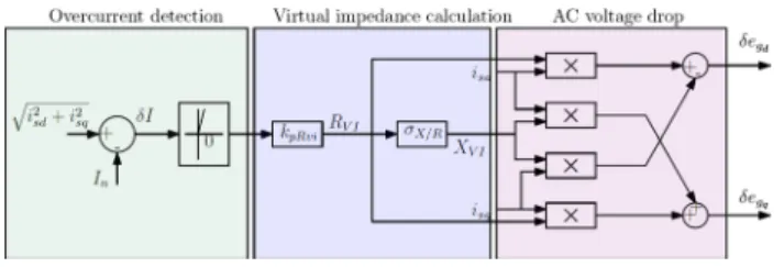
limitation has to be implemented. Since direct AC voltage control does not possess a current servo-controller to limit current transients, the threshold virtual impedance (TVI) depicted in Fig. 10 is adopted.
As illustrated in Fig. 10, the TVI operation principle is divided into three main phases.
• Overcurrent detection and activation, i.e., activation only when the current exceeds In= 1 p.u.
• Virtual impedance calculation. • AC voltage drop calculation.
The expressions of XVI and RVI are given in (18a) and
(18b), respectively.
where 𝛿I = Is− In.kpRVI and 𝜎X∕R are defined as the virtual
impedance proportional gain and the virtual impedance ratio, respectively.
The parameter kpRVI is tuned to limit the current
magni-tude to a suitable level Imax during overcurrent, while 𝜎X∕R
ensures a good system dynamics during overcurrent. The tuning method of these parameters is explained in [25].
When the virtual impedance is activated, new AC volt-age references are given by (19) and (20):
The effect of the virtual impedance on the system depends mainly on the voltage loop dynamics. Therefore, a direct feedforward on the modulated voltage vmdq can be added [2]. A block diagram of the direct AC voltage con-trol embedded in the TVI is depicted in Fig. 11.
(18a) XVI=
{k
pRVI𝜎X∕R𝛿I if 𝛿I > 0
0 if 𝛿I≤ 0 (18b) RVI= XVI∕𝜎X∕R (19) e∗gd= Eset+ ( qmes 1 1+ TQs− q ∗ ) np− 𝛿egd (20) e∗gq= −𝛿eg q.
In the following, the TVI parameters are set to Imax = 1.2 p.u, kpRVI = 1.31 p.u and 𝜎X∕R= 3.
4 Simulation results
In this section, several case studies are used to evaluate the developed control. The case studies cover several pro-totypical scenarios based on single-inverter and multi-inverter systems.
4.1 Single inverter connected to a grid
In addition to the AC voltage dynamics, which are already demonstrated in Fig. 8, this subsection focuses on the system behavior in the case of a fault.
4.1.1 Symmetrical three‑phase short circuit
A symmetrical three-phase bolted fault is applied to the system at the PCC level as depicted in Fig. 12. At t = 1s , a
Fig. 11 Block diagram of the direct AC voltage control embedded in the current limitation algorithm
Fig. 12 Single inverter subjected to a three-phase short-circuit
150ms fault occurred. Simulation results are gathered and presented in Fig. 13.
As can be seen from Fig. 13, the AC voltage drops to zero during the fault, which leads to an increase in the VSI output current. The output current amplitude Is reaches 1.65 p.u in
the first 10 ms. Then, it is limited to its maximum allowable value Imax = 1.2 p.u during the rest of the fault duration. Once the fault is cleared, the system recovers stably to its operating point within 300 ms.
4.1.2 Phase shift
Continuing with the system shown in Fig. 12, a phase shift of 30° is applied to the system at t = 1s as shown by the grid voltage vg in Fig. 14. During the phase shift, the current
increase is limited to Imax . Then, the system recovers to its operating point in a stable manner.
4.2 Three‑bus system case study
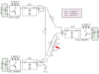
In future power systems, grid-forming inverters of different ratings will be interconnected via transmission lines with diverse topologies. To study the behavior of a system and the performances of the developed control in such a scenario, the simple meshed grid of 320 kV illustrated in Fig. 15 is used. The studied system consists of overhead lines, i.e., L1= 25 km , L2= 4L1 and L3= 5L1 , a three-phase resis-tive load, and a three-bus system as shown in Fig. 15. The switching effect of the power inverters is taken into account. The LCL filter design of each inverter depends on its rated power as indicated in the downstairs of each inverter in Fig. 15 and the per-unit values listed in Table 1.
Simulation results for the following test cases show the local AC signals of each power inverter, i.e., AC voltage across the capacitors, output current of the LCL filter, active power and reactive power.
4.2.1 P‑Load change
Initially, the system is at no load Pload= 0W . Then, a load
change of Pload= 1125MW is applied at t = 0.5s.
As shown in Fig. 16, the load change leads to a voltage transient in all of the VSIs. The AC voltage drop during the load connection depends on the electrical distance between the VSIs and the load, i.e., since VSI2 is far from the load
location, the transient AC voltage drop is more important than VSI1 and VSI3 . Based on the proposed control, the AC
voltage has an overshoot of 0.7% after the load connection and recovers stability to its nominal value within 80ms.
Fig. 14 System behavior subjected to a phase shift of 30°
Fig. 15 Three-bus system-based grid-forming inverters
4.2.2 AC voltage amplitude change
Initially, a resistive load of Pload= 1125MW is connected
and the power inverters are driven to there nominal AC volt-age EgVSC123 = 1pu . Then, a -10% AC voltage amplitude is applied on VSI1 at t = 2s as shown in Fig. 17.
The AC voltage dynamics of VSI1 corresponds to the
one defined in the specifications, i.e., Tr= 200ms . The AC
voltage change results in a reactive power change with the same dynamics, as well as a low transient coupling with the active power as expected. For VSI2 and VSI3 , this
change is seen as an external disturbance leading to an AC voltage transient due to the reactive power exchange between the VSIs. At t = 3.25s , the AC voltage of VSI1
recovers its nominal value with same dynamics.
4.2.3 Symmetrical three‑phase short circuit followed by line tripping
A 400-ms symmetrical three-phase short circuit has occurred between two lines as depicted in Fig. 18. Then, it is cleared by tripping the lines using the switch K1 . In this
test case a Pload of 1125MW is assumed to be connected.
As shown in Fig. 18, when a fault occurs, the AC volt-ages drop by 50% for VSI2 and 60% for VSI1−3 . As a result,
it should be noticed that the output current Ig reaches 1.65
p.u in first 30 ms. Then, the output currents of all of the inverters are limited to 1.2 p.u. Once the fault is cleared, the system recovers stably to its operating point within 50 ms.
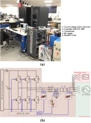
5 Experimental results
The developed control is validated on a small-scale experi-mental bench like the one illustrated in Fig. 19(a). The power inverter is supplied by an ideal DC voltage source of 600 V and connected to a 300 V ph–ph AC grid through an LCL filter as presented in this paper and shown in
Fig. 17 System dynamics following an AC voltage change
Fig. 18 System behavior during a symmetrical three-phase short cir-cuit followed by a tripping line
Fig. 19 Experimental bench: a mockup presentation; b functional schema
Fig. 19(b). The switching frequency of the converter is fsw= 10kHz , and a DSPACE1005 is used as the controller with a time step of 40 μs.
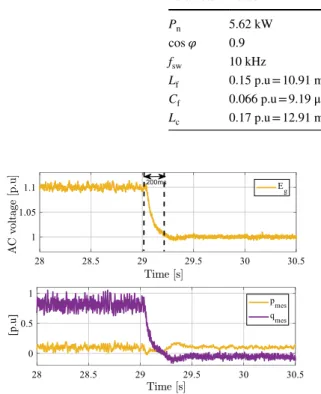
The mockup parameters are listed in Table 7. The parameter of the LCL filter approximatively corresponds to those used in the paper in per unit, i.e., Table 1. The control parameters are those listed in Table 3.
Two possible experimentations have been completed based on the developed control, i.e., the grid-connected mode where the VSI is connected to the laboratory power system ( Kg is closed), and the autonomous mode where the
VSI is connected to a three-phase variable resistive load ( KL
is closed).
5.1 Grid‑connected mode
Similar to the test case shown in Fig. 8, the test case shown in Fig. 20 first brings the system to the steady state with an AC voltage of Eg = 1.1 p.u before it is stepped back to 1.0
p.u.
The experimental results in Fig. 20 support the analysis done in this paper where the AC voltage dynamics respect the imposed specifications, i.e., Tr5% = 200ms and the tran-sient coupling between the AC voltage and the active power is very small.
5.2 Standalone mode
Grid-forming inverters should remain stable regardless of the grid topology and based on the same control law. This subsection aims to show the effectiveness of the developed control in operating in the standalone mode.
The power inverter is now connected to a variable resis-tive load of Pload= 4kW . In Fig. 21, load changes of 0.2 p.u
and 0.4 p.u have been applied. The results show that the VSI feeds the load in a stable manner and represents a very weak AC voltage transient.
In Fig. 22, an AC voltage amplitude change of 10% occurs. The obtained results show that the AC voltage dynamics respect the response time specifications in the autonomous mode as in the grid-connected mode.
These simple test cases aim to show the flexibility of the developed control and its ability to operate in various grid topologies, as well as its ability to achieve higher dynamic performances than the conventional cascaded control.
6 Conclusions
This paper proposes a direct AC voltage control structure and its controller tuning for grid-forming inverters. Despite the fact that the state-feedback control technique is consid-ered as a conventional one, this paper demonstrates that its
Table 7 System parameters Parameter Value
Pn 5.62 kW cos 𝜑 0.9 fsw 10 kHz Lf 0.15 p.u = 10.91 mH Cf 0.066 p.u = 9.19 μF Lc 0.17 p.u = 12.91 mH
Fig. 20 AC voltage change and its impact on active power
Fig. 21 Resistive load change
application to the grid-forming inverters in high-power system applications has many advantages when compared to the cas-caded control structure, especially in terms of dynamics. The proposed tuning method for controller gains has allowed for achieving the desired AC voltage response time, while taking into account the coupling issues with the active power.
The fundamental issue with using direct AC voltage control is its inability to protect inverters against overcurrent. Thus, this paper combines AC voltage control with threshold virtual impedance. The choice of this solution is motivated by the ease of its implementation. Moreover, it does not have any impact on the system behavior under normal operation. The effective-ness of the proposed control is demonstrated in a number of test cases by time domain simulations and experiments.
Acknowledgements This project has received funding from the Euro-pean Union’s Horizon 2020 research and innovation program under grant agreement No 691800. This paper reflects only the author’s views, and the European Commission is not responsible for any use that may be made of the information it contains.
Appendix
Augmented state-space control matrices: xT=
[
Δisd Δisq Δegd Δegq Δigd ΔigqΔ𝜁dΔ𝜁q… Δ𝛿ΔpmesΔqmes ] Aaug 11= ⎡ ⎢ ⎢ ⎢ ⎢ ⎣ −Rf 𝜔b Lf +𝜔bK11 Lf 𝜔𝜔b+ 𝜔bK12 Lf −𝜔b Lf +𝜔bK13 Lf −𝜔𝜔b+𝜔bK21 Lf −Rfpu𝜔b Lf +𝜔bK21 Lf +𝜔bK21 Lf 𝜔b Cf 0 0 ⎤ ⎥ ⎥ ⎥ ⎥ ⎦ Aaug 12= ⎡ ⎢ ⎢ ⎢ ⎢ ⎢ ⎢ ⎢ ⎣ 𝜔bK14 Lf 𝜔bK15 Lf 𝜔bK16 Lf − 𝜔bKI11 Lf − 𝜔bKI12 Lf −𝜔b Lf + 𝜔bK21 Lf 𝜔bK21 Lf + 𝜔bK21 Lf − 𝜔bKI21 Lf − 𝜔bKI21 Lf 𝜔𝜔b −𝜔b Cf 0 0 0 0 0 −𝜔b Cf 0 0 0 −Rc 𝜔b Lc 𝜔𝜔b 0 0 ⎤ ⎥ ⎥ ⎥ ⎥ ⎥ ⎥ ⎥ ⎦ Aaug13= [0]3×3 ATaug 21= ⎡ ⎢ ⎢ ⎢ ⎣ 0 0 0 0 0 0 0 0 𝜔b Cf 0 0 0 0 0 0 0 −𝜔𝜔b 𝜔b Lc 0 1 0 0 𝜔cIg d0 −𝜔cIgq0 ⎤ ⎥ ⎥ ⎥ ⎦
References
1. Erlich, I., et al.: New control of wind turbines ensuring stable and secure operation following islanding of wind farms. IEEE Trans. Energy Convers. 32(3), 1263–1271 (2017)
2. Denis, G., Prevost, T., Debry, M., Xavier, F., Guillaud, X., Menze, A.: The Migrate project: the challenges of operating a transmis-sion grid with only inverter-based generation. A grid-forming control improvement with transient current-limiting control. IET Renew. Power Gener. 12(5), 523–529 (2018)
3. Erlich, I.: Control challenges in power systems dominated by con-verter interfaced generation and transmission technologies. In: NEIS 2017; Conference on Sustainable Energy Supply and Energy Storage Systems, pp. 1–8 (2017)
4. Rocabert, J., Luna, A., Blaabjerg, F., Rodríguez, P.: Control of power converters in AC microgrids. IEEE Trans. Power Electron. 27(11), 4734–4749 (2012)
5. Judewicz, M.G., González, S.A., Fischer, J.R., Martínez, J.F., Car-rica, D.O.: Inverter-side current control of grid-connected voltage source inverters with LCL filter based on generalized predictive control. In: IEEE J. Emerg. Sel. Top. Power Electron., vol. 6, no. 4, pp. 1732–1743 (2018)
6. Hamed, H.A., Abdou, A.F., Acharya, S., Moursi, M.S.E., EL-Kholy, E.E.: A novel dynamic switching table based direct power control strategy for grid connected converters. In: IEEE Trans. Energy Convers., vol. 33, no. 3, pp. 1086–1097 (2018)
7. Hannan, M.A., Ghani, Z.A., Mohamed, A., Uddin, M.N.: Real-time testing of a fuzzy-logic-controller-based grid-connected photovoltaic inverter system. IEEE Trans. Ind. Appl. 51(6), 4775–4784 (2015)
8. Chen, D., Zhang, J., Qian, Z.: An improved repetitive control scheme for grid-connected inverter with frequency-adaptive capa-bility. IEEE Trans. Ind. Electron. 60(2), 814–823 (2013)
Aaug 22= ⎡ ⎢ ⎢ ⎢ ⎢ ⎢ ⎢ ⎢ ⎢ ⎢ ⎢ ⎢ ⎣ 0 0 −𝜔b Cf 0 0 0 −Rc 𝜔b Lc 𝜔𝜔b 0 0 𝜔b Lc −𝜔0𝜔b − Rc 𝜔b Lc 0 0 0 0 1 0 0 1 0 0 0 0 0 0 0 0 0 𝜔cIg q0 𝜔cEgd0 𝜔cEgd0 0 0 𝜔cIg d0 𝜔cEgq0 −𝜔cEgd0 0 0 ⎤ ⎥ ⎥ ⎥ ⎥ ⎥ ⎥ ⎥ ⎥ ⎥ ⎥ ⎥ ⎦ Aaug 23= ⎡ ⎢ ⎢ ⎢ ⎢ ⎢ ⎢ ⎢ ⎢ ⎢ ⎢ ⎣ 0 0 0 Vpccd0sin(𝛿0)𝜔b Lc −𝜔bIgq0 0 Vpccd0cos(𝛿0)𝜔b Lc 𝜔bIgd0 0 0 0 0 0 0 0 0 −mp 0 0 −𝜔c 0 −𝜔c 0 0 ⎤ ⎥ ⎥ ⎥ ⎥ ⎥ ⎥ ⎥ ⎥ ⎥ ⎥ ⎦
9. Fu, X., Li, S.: Control of single-phase grid-connected converters with LCL filters using recurrent neural network and conventional control methods. IEEE Trans. Power Electron. 31(7), 5354–5364 (2016)
10. Li, Z., Zang, C., Zeng, P., Yu, H., Li, S., Bian, J.: Control of a grid-forming inverter based on sliding-mode and mixed $H_2/H_ınfty $ control. IEEE Trans. Ind. Electron. 64(5), 3862–3872 (2017) 11. D’Arco, S., Suul, J.A., Fosso, O.B.: Automatic tuning of cascaded
controllers for power converters using eigenvalue parametric sen-sitivities. IEEE Trans. Ind. Appl. 51(2), 1743–1753 (2015) 12. Qoria, T, Gruson, F. Colas, F., Guillaud, X., Debry, M., Prevost,
T.: Tuning of cascaded controllers for robust grid-forming voltage source converter. In: 2018 Power Systems Computation Confer-ence (PSCC), pp. 1–7 (2018)
13. Qoria, T., et al.: Tuning of AC voltage-controlled VSC based linear quadratic regulation. In: IEEE Milan PowerTech, pp 1–6. Milan, Italy (2019)
14. Vinifa, R., Kavitha, A.: Linear quadratic regulator based current control of grid connected inverter for renewable energy appli-cations. In: 2016 International Conference on Energy Efficient Technologies for Sustainability (ICEETS), pp. 106–111 (2016) 15. Shao, R., Yang, S., Wei, R., Chang, L.: Advanced current control
based on linear quadratic regulators for 3-phase grid-connected inverters. In: 2015 IEEE 6th International Symposium on Power Electronics for Distributed Generation Systems (PEDG), pp. 1–5 (2015)
16. Denis, G.: From grid-following to grid-forming: The new strategy to build 100% power-electronics interfaced transmission system with enhanced transient behavior. Ph.D thesis, Ecole centrale de Lille (2017)
17. Qoria, T., Gruson, F., Colas, F., Denis, G., Prevost, T., Guillaud, X.: Inertia effect and load sharing capability of grid forming con-verters connected to a transmission grid. In: 15th IET Interna-tional Conference on AC and DC Power Transmission (ACDC 2019), pp. 1–6 (2019)
18. D’Arco, S., Suul, J.A.: Equivalence of virtual synchronous machines and frequency-droops for converter-based microGrids. IEEE Trans. Smart Grid 5(1), 394–395 (2014)
19. Liu, J., Miura, Y., Ise, T.: Comparison of dynamic characteris-tics between virtual synchronous generator and droop control in inverter-based distributed generators. IEEE Trans. Power Elec-tron. 31(5), 3600–3611 (2016)
20. Bajracharya, C., Molinas, M., Suul, J.A., Undeland, T.M.: Under-standing of tuning techniques of converter controllers for VSC-HVDC. In: Proc. of Nordic Workshop on Power and Industrial Electronics, NORPIE 2008, Espoo, Finland, 9–11 June (2008) 21. Denis, G., Prevost, T., Panciatici, P., Kestelyn, X., Colas, F.,
Guil-laud, X.: Improving robustness against grid stiffness, with internal control of an AC voltage-controlled VSC. In: 2016 IEEE Power and Energy Society General Meeting (PESGM), pp. 1–5 (2016) 22. Kemin, Z., John, C. D., Keith, G.: Robust and optimal control.
ISBN: 0134565673, 9780134565675 (1996)
23. Sirisha, C.: Design and implementation: linear quadratic regu-lator. LAP Lambert Academic Publishing. ISBN: 3846556432, 9783846556436 (2011)
24. Danielsen, S., Fosso, O.B., Toftevaag, T.: Use of participation factors and parameter sensitivities in study and improvement of low-frequency stability between electrical rail vehicle and power supply. In: 2009 13th European Conference on Power Electronics and Applications, pp. 1–10 (2009)
25. Paquette, A.D., Divan, D.M.: Virtual impedance current limiting for inverters in microgrids with synchronous generators. IEEE Trans. Ind. Appl. 51(2), 1630–1638 (2015)
Taoufik Qoria received his M.S. degree in Electrical Engineering for Sustainable Development from Lille 1 University of Sci-ence and Technology, Villeneuve d’Ascq, France, in 2016. Since 2016, he has been working on the modeling and control of the power inverters in HVDC and HVAC applications. He is pres-ently working toward his Ph.D. degree at ENSAM ParisTech in the Laboratory of Electrical Engineering and the Power Elec-tronics of Lille (L2EP), Lille, France, which is funded by the European project H2020 MIGRATE. His current research interests include the massive integration of power electronic devices in power transmission systems.
Chuanyue Li (S’16) received his B.S. degree in Electrical and Electronic Engineering from both Cardiff University, Cardiff, WLS, UK, and the North China Electric Power University, Bei-jing, China, in 2013; and his Ph.D. degree in Electrical and Electronic Engineering from Cardiff University, in 2017. He is a Postdoctoral Scholar at the Laboratory of Electrical Engi-neering and Power Electronics (L2EP), Lille, France. His cur-rent research interests include HVDC control and protection, and power electronics.
Ko Oue was born in Hiroshima, Japan. He received his B.S. and M.S. degrees in Electrical Engi-neering from Doshisha Univer-sity, Kyoto, Japan, in 2017 and 2019, respectively. He received his M.S. degree from Ecole Cen-trale of Lille, Villeneuve-d’Ascq, France, in 2018.