2D-photochemical model for forbidden oxygen line emission for comet 1P/Halley

(1)

2D-photochemical model for forbidden oxygen line

emission for comet 1P/Halley

G. Cessateur,

1⋆

_{J. De Keyser,}

1

_{R. Maggiolo,}

1

_{M. Rubin,}

2

_{G. Gronoff,}

3

_{A. Gibbons,}

1,4

E. Jehin,

5

F. Dhooghe,

1

H. Gunell,

1

N. Vaeck

4

and J. Loreau

4

1_{Space Physics Division, Royal Belgian Institute for Space Aeronomy, Ringlaan 3, B-1180 Brussels, Belgium}

2_{Physikalisches Institut, University of Bern, Sidlerstr. 5, CH-3012 Bern, Switzerland}

3_{Science Directorate, Chemistry and Dynamics Branch, NASA Langley Research Center, Hampton, Virginia USA; SSAI, Hampton, Virginia USA}

4_{Service de Chimie Quantique et Photophysique, Universit´}_{e Libre de Bruxelles, Av. F. D. Roosevelt 50, B-1050 Brussels, Belgium}

5_{Institut d’Astrophysique, de G´}_{eophysique et Oc´}_{eanographie, Universit´}_{e de Li`}_{ege, All´}_{ee du 6 aoˆ}_{ut 17, 4000 Li`}_{ege, Belgium}

Accepted XXX. Received YYY; in original form ZZZ

ABSTRACT

We present here a 2D-model of photochemistry for computing the production and loss mechanisms of the O(1_{S) and O(}1_{D) states, which are responsible for the emission lines at 577.7 nm, 630 nm,}

and 636.4 nm, in case of the comet 1P/Halley. The presence of O₂ within cometary atmospheres, measured by the in-situ ROSETTA and GIOTTO missions, necessitates a revision of the usual photochemical models. Indeed, the photodissociation of molecular oxygen also leads to a significant production of oxygen in excited electronic states. In order to correctly model the solar UV flux absorption, we consider here a 2D configuration. While the green to red-doublet ratio is not affected by the solar UV flux absorption, estimates of the red-doublet and green lines emissions are, however, overestimated by a factor of two in the 1D model compared to the 2D model. Considering a spherical symmetry, emission maps can be deduced from the 2D model in order to be directly compared to ground and/or in-situ observations.

Key words: comets: general – methods: numerical – molecular processes

1 INTRODUCTION

Comets are usually considered as the best preserved ob-jects in the solar system since its formation 4.6 billion years ago. Their study could bring us valuable information re-garding the composition of the primitive solar nebula. The recent discoveries of the Rosetta mission, currently orbiting around the comet 67P/Churyumov-Gerasimenko (hereafter 67P) (Glassmeier et al. 2007), have shed a new light on our current knowledge regarding cometary composition. Specifi-cally, the presence of molecular oxygen in the inner coma, in significant abundances relative to water (3.80 ± 0.85% for 67P) was reported by Bieler et al. (2015) measured by the Rosetta Orbiter Spectrometer for Ion and Neutral Analy-sis (ROSINA,Balsiger et al.(2007)). The presence of O2has

also been confirmed with a reinterpretation of the Giotto data obtained during the flyby of the comet 1P/Halley (Rubin et al. 2015), with a 3.7 ± 1.7% abundance relative to water. These results strongly suggest that molecular oxygen is in fact a common species in cometary atmospheres. Cur-rent modeling of the oxygen line emissions therefore has to be revised, in order to take the presence of molecular oxygen into account.Cessateur et al.(2016) explored the impact of

⋆ _{E-mail: gael.cessateur@aeronomie.be}

the presence of molecular oxygen on the red-doublet (at 630 and 636.4 nm) and green (at 577.5 nm) line emissions for 67P. In this paper we perform a similar study for the comet 1P/Halley and we extend the model by considering a 2D approach.

The excited oxygen states come mainly from the pho-todissociation of H2O, CO2, O2 and CO as suggested

both by remote observations of atomic oxygen lines (see e.g. McKay et al. 2015; Decock et al. 2015), and by mod-eling (see e.g.Bhardwaj & Raghuram 2012, and references therein). The oxygen states of interest are O(1

D) (leading to emissions at 630 and 636.4 nm), and O(1

S) with a deac-tivation towards the oxygen state O(1

D) through radiative emission at 557.7 nm. We will focus on the impact of the presence of O2 on the green to red-doublet emission

inten-sity ratio (G/R) as a function of the cometocentric distance, traditionally used to determine the abundances of the ma-jor oxygen-bearing volatile components in cometary atmo-spheres (Decock et al. 2015), in the case of 1P/Halley. After briefly introducing the 1D photochemical model used for 67P to assess the red-doublet and green line emissions, we will focus on a 2D approach in order to better take the solar UV flux absorption into account. Using a spherical symme-try, emission maps according to different observation angles can be deduced from the 2D model. We furthermore discuss

at Bibliotheque Fac de Medecine on September 8, 2016

http://mnras.oxfordjournals.org/

(2)

tral cometary atmosphere, we consider here the result of the DSMC model presented by Rubin et al. (2011), giving the number densities and velocities of the main species as a function of cometocentric distance r, starting from the sur-face at r = 6 km outward, for a water production, Qp, of

7.1029

s−1 _{and for a heliocentric distance of 0.90 AU. From}

this spherically symmetric neutral model, we estimate the number densities of the O(1

D) and O(1

) states, Ni, within

the cometary atmosphere by solving the continuity equation assuming spherical symmetry:

1 r2 d dr(r 2 Niv(r)) = Pi−Li, (1)

where Pi is the production term, Li the loss term and

v(r) the velocity of the excited oxygen atom. The dominant source of O(1

D) and O(1

S) states is the photodissociation by the solar UV flux of the oxygen-bearing volatile compo-nents as discussed byDecock et al.(2015). We consider here the usual species such as H2O, CO2, and CO. In the case

of 67P (see Cessateur et al. 2016), this list of species had to be completed with O2, which has been detected in

sig-nificant abundance (3.80 ± 0.85% relative to water) within the cometary atmosphere of 67P (Bieler et al. 2015). A new interpretation of the Giotto data has been performed to in-vestigate the presence of O2 during the 1P/Halley flyby in

1986.Rubin et al.(2015) demonstrate the presence of molec-ular oxygen with a significant abundance of about 3.7 ± 1.7% relative to water using the data from the Neutral Mass Spectrometer (NMS, Krankowsky et al. (1986) ) on board the Giotto spacecraft (Reinhard 1986). This makes molec-ular oxygen the third most abundant species behind water and CO (13.1% relative to water), and before CO2 (2.5%

relative to water) for 1P/Halley. However, the DSMC model from Rubin et al. (2011) does not provide the velocity for O2, but it does so for methanol (CH3OH) which has a

sim-ilar molar mass as O2. The radial profiles for these four

species are displayed in Fig. 1. The reaction rates for the photodissociation due to the solar UV flux are computed for each altitude within the cometary atmosphere. Because of the solar UV flux absorption, reaction rates are indeed not constant.

Regarding the loss reactions, we consider collisions and ra-diative decay (which produce the green and red-doublet emissions we are interested in). Given the neutral densities for 1P/Halley, the loss reactions for O(1

D) are dominated by collisions with water for altitudes lower than 1000 km, while radiative decay leading to emissions at 630 and 636.4 nm dominates at higher altitudes. For the O(1

S) states, col-lisions with water are predominant below 100 km, while

ra-Figure 1. Number densities considered based on the DSMC

model from Rubin et al. (2011), for water (red), CO (blue),

O2 (black), and CO2 (green) using a water production rate of

7×1029_s−1_{at 0.90 AU heliocentric distance. The computed}

num-ber densities for O(1

D) (dashed black line) and for O(1

S) (dash-dotted black line) are also displayed.

diative decay at 577.7 is dominating above. The different loss reactions rates considered here are summarized in Ta-ble 2 fromCessateur et al.(2016).

The number densities for O(1_{D) and O(}1_{S) are usually}

com-puted over a radial profile, from 10 km above the nucleus to a maximum limit of integration, R, equal to 106

km here. Figure1displays these number densities for 1P/Halley along with the neutral densities. These number density profiles are computed for the situation where the observer is located be-tween Sun and comet. As primary input, the solar UV flux is characterized here by the solar activity as expressed by the F10.7 proxy of 104, already considered by Cessateur et al.

(2016) in case of 67P, but here for a heliocentric distance of 0.90 AU. Volumetric emission profiles for the red-doublet and green line can then be deduced by multiplying the num-ber densities of O(1

D) and O(1

S) with the Einstein transi-tion probabilities, 8.58 ×10−3_s−1_{and 1.26 s}−1_{, respectively.}

The resulting profiles are then usually projected over a line-of-sight at various projected distances, z (see Eq. 9 from

Bhardwaj & Raghuram 2012), resulting in a 1.5D model as displayed in Fig. 2. By doing so, this approach considers that the solar UV flux absorption is symmetrical to the po-sition of the nucleus. For a line-of-sight at 10 km above the nucleus, the estimated red-doublet and green line emissions are of about 17626 R and 7717 R, respectively, using this approach. For a higher altitude, at 100 km above the nu-cleus, the estimated emissions are of about 17938 R and 7882 R. However, in the case of 1P/Halley, neutral densities around the nucleus are high enough to completely absorb the solar UV flux. The problem is then no longer symmet-rical to the nucleus, and we cannot use projections of the O(1

D) and the O(1

S) radial profiles from Fig. 1. A more complete model then has to be defined: a 2D model con-sidering 1135x1136 parallel lines of sight through the coma, using an adaptive mesh grid for the spatial resolution. This allows us to consider proper line of sight for various altitudes

(3)

Figure 2. Computed emission brightness (in Rayleigh) for 1P/Halley along a projected distance from the nucleus using the 1.5D model (dashed lines) and the 2D model (thick lines) for green and red-doublet emissions, in black and red lines, respectively.

from the cometocentric distance and not the projected ones from Fig.1as for the 1.5D model. In this case, the estimated emissions at 10 km above the nucleus are of about 8836 R and 3842 R, as displayed in Fig.2. The estimated emissions are overestimated by a factor of two while using the com-mon approach with a symmetrical system. The 1.5D model approximation can be justified for comets with a very low water production rate, but not for very active comets such as 1P/Halley. In the following, we will consider then the full 2D model, by carefully taking into account the solar UV flux absorption along the different lines of sight.

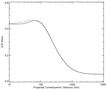
We also consider the green to red-doublet emission inten-sity ratio (G/R) as a function of the cometocentric distance, which is usually used as proxy for determining the CO2

abundances in cometary atmospheres (see e.g.Decock et al. 2015), and more recently also to constrain the O2abundance

(Cessateur et al. 2016). The G/R ratio for 1P/Halley is dis-played in Fig. 3 for both 1.5D and 2D models. Both G/R ratio profiles present a local maximum for altitudes around 70 km for the 2D model while it is close to 60 km for the 1.5D model. In general, there is a slight difference for the G/R ratio for altitudes lower than 200 km. The most im-portant deviation occurs for an altitude range between 20 and 50 km, where the 1.5D model gives slightly higher G/R ratio values than the 2D model with a difference of about 0.02 in average. For the G/R ratio, the 1.5D model seems to be a good approximation. The 2D model is, however, nec-essary when calculating the absolute values of the oxygen lines emissions.

3 EMISSION MAPS

For a spherical symmetry, the 2D model can be modified to produce emission maps, which are better tools for a direct comparison with ground and in-situ observations than aver-aged radial profiles. The resulting 2.5D model can thus be used to simulate observations made from different viewing

Figure 3.G/R ratio profile for 1P/Halley from 10 to 104_{km for}

a line of sight crossing the projected cometocentric distance for the 1.5D (dashed line) and 2D (thick line) models.

angles with respect to the comet and the Sun. We consider a x, y, z Cartesian coordinate system, with the comet nu-cleus and the Sun located at the (0,0,0) and (0,0,+0.90 AU) positions, respectively.

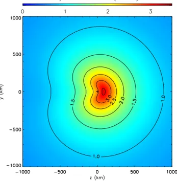
3.1 Comet-Sun-Observer in opposition

We start with the traditional viewing geometry, when the Sun, the comet and the observer are aligned (i.e. the ob-server located on the z-axis with positive value lower than 0.90 AU). Figure 4 displays the red-doublet emission map around the nucleus: along the direction y = 0, from 6 to 5000 km on the x-axis, the profile corresponds to the red thick line from Fig. 2. The red-doublet emissions reach a maximum for an altitude of 485 km with 15721 R. The in-tensity profile decreases for lower altitudes since the solar UV flux is more absorbed close to the nucleus: the emis-sions are indeed reduced down to 3927 R at 10 km above the nucleus. Regarding the green line emissions, the overall profile is very similar as for the red-doublet line emissions, but with a maximum reached for an altitude of 115 km with 5277 R. As for the line emissions, the G/R ratio follows the spherical distribution, so the results will not be different as the ones presented in Fig.3, with a G/R ratio maximum of 0.461 over a ring at roughly 70 km above the nucleus.

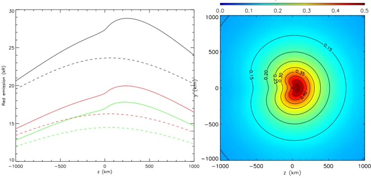
3.2 Comet-Sun-Observer in quadrature

We now consider an angle of 90◦ _{between the comet, the}

Sun and the observer located on the x-axis, with values that exceed the coma dimensions considered here (between -106

and 106

km). The resulting emission maps for the red-doublet and green line emissions are displayed in Fig.5. Because of the strong solar UV flux absorption by the neutral species, emission maps are not symmetric anymore. Emissions for red-doublet lines reach their maximum levels (> 17.81 kR) for a region at z = [180:220 km] and y =[-50:50 km]. This region is a signature for the 1P/Halley comet. By

(4)

Figure 4.Emission map for the red-doublet line when the comet, the Sun, and the observer are in opposition. The dashed line rep-resents the maximum iso-emission line.

comparing with the region located at z = [-220:-180 km] where emissions are of about 16.5 kR, there is a difference of over 1 kR. Further away from the nucleus, between z = -500 km and z = 500 km, the difference is now over 2 kR. Such large differences are probably detectable with current ground-based instruments The emission distribution is different from the traditional viewing geometry. Looking at two different angles of observations might then help to better constrain the atmospheric models. We obtained similar trends for the green line emissions, with an emission maximum of about 7.76 kR, for a region around z = 100 km. For z=-100 km, emissions are estimated of about 4.5 kR. The difference is then higher than for the red-doublet line emissions ( 3 kR compared to 2 kR), but occurs on smaller spatial scales, making it harder to detect.

We can also look at the G/R ratio, displayed in Fig. 6, for altitudes lower than 500 km. The G/R ratio profile here is an increasing function towards the nucleus. The G/R ratio maximum is lower here compared to the opposition view, with 0.41 for the space region located at z = [30:100 km] and y=[-20:20 km], compared to 0.461 over a ring at 70 km distance from the nucleus. Those differences can also help to constrain the different species abundances in the case of very active comets such as 1P/Halley. Observations of such comets, however, need to focus on regions close to the nucleus, typically within 100 km.

4 DISCUSSION The production of the O(1

D) and O(1

S) oxygen states, and therefore the G/R ratio, is affected by several parameters such as the different species abundances, the water

produc-Figure 5. Emission maps for the red-doublet (top figure) and

green (bottom figure) lines for a quadrature view between the comet, the Sun, and the observer. The comet location is repre-sented by a black cross.

tion rate Qp, and the out-gassing speed, v. As primary

pa-rameters, the knowledge of the cross sections for the different species is also a critical parameter. All these parameters af-fect the absorption of the solar UV flux within the cometary atmospheres.

4.1 Water production rates

The water production rate, Qp, is a critical parameter for

determining the atmospheric neutral densities. It is thus

(5)

Figure 6.Green to Red ratio for a quadrature view between the comet, the Sun, and the observer. The comet location is repre-sented by a black cross.

teresting to look at how this parameter affects the produc-tion of the O(1

D) and O(1

S) oxygen states through the ab-sorption of the solar UV flux. We still consider the model fromRubin et al. (2011) originally designed for 1P/Halley, considering the same volatiles composition and out-gassing speeds but varying the water production rate. We then com-pare the outcomes of the 1.5D model to the 2D model, and this for several altitudes. Figure7displays the ratio 2D/1.5D for the red-doublet and green line emissions for a line of sight 10 km, 100 km, and 1000 km above the nucleus, considering the traditional viewing geometry.

For the sake of comparison, we consider several comets char-acterized by their water production rates (and not by com-position), for a heliocentric distance close to 0.90 AU, such as the 73P-C/Schwassmann-Wachmann 3 comet (Qp= 1.7

× ₁₀28 _s−1_, _{Decock et al.} ₍₂₀₁₅_{)), the C/1996 B2}

Hyaku-take comet (Qp = 2.2 × 1029 s−1,Bhardwaj & Raghuram

(2012)) and the C/1995 O1 (Hale-Bopp) comet (Qp = 9.6

×₁₀29_s−1_,_{Dello Russo et al.}₍₂₀₀₀_{)). We also consider the}

comet 67P, with Qp = 4 × 10 27

s−1_{, but for a heliocentric}

distance of 1.25 AU where 67P was at its perihelion in Au-gust 2015. In the case of observations at 10 km above the nucleus, the 2D/1.5D ratio is 0.5 for water production rates greater than 1.5 × 1029

s−1_{, which includes 1P/Halley and}

Hyakutake. The ratio of 0.5 represents a saturation limit, where the solar UV flux has been completely absorbed. For production rates lower than 1 × 1027

s−1_{, the solar UV flux is}

not absorbed significantly enough to impact the green and red-doublet emissions. The 67P comet is slightly affected with a difference of about 5%. For an altitude of 100 km, the ratio for 1P/Halley is about 0.65, while for Hyakutake it is 0.85. For 67P and 73P-C, the difference between the 2D and 1.5D models is negligible. For higher altitudes, at 1000 km above the nucleus, only the green and red-doublet emissions for 1P/Halley are affected by the solar UV flux

absorption, with a ratio of 0.96, also depicted in Fig.2. It is important to note that these results are correct when considering the composition of the 1P/Halley comet. Indeed, the relative abundances of CO, CO2and O2differ from those

of 1P/Halley for the different comets taken as examples. The 2D/1.5D ratio profiles would then change slightly but the overall picture would remain the same. Indeed, the CO2and

CO abundances are quite similar for the four comets ([1%-8%] for CO2, [5%-22%] for CO), and the water is the major

responsible for the solar UV flux absorption. This strongly suggests that a 2D model such as developed here, is neces-sary for various cometary activities above Qp = 1 × 1027

s−1 _{for calculations close to the nucleus.}

4.2 Outgassing speed

In the previous subsections, only the water production rate was varied, leaving the composition and outgassing speeds unaffected. This latter parameter is however critical in the neutral distribution along a radial profile. The Haser model is traditionally used to provide a simple neutral atmosphere (Haser 1957). However, a constant outgassing speed is of-ten considered along the radial profile, with typical val-ues ranging from 700 m.s−1 _{(e.g. for 67P) to 800 m.s}−1

(e.g. for Hyakutake). The DSMC model results presented byRubin et al.(2011) provide, however, the outgassing ve-locity as a function of the distance to the nucleus. Due to the gas expansion the bulk velocity of the parent water molecule ranges from 200 to 700 m s−1 _{for altitudes lower than 100}

km, as displayed in Fig.8. The velocities of the other neutral species are very similar to those of water due to collisional coupling of the neutral species in the innermost part of the coma. For a constant water production rate, Qp = 7.2 ×

1029

s−1_{, the water density for the 1P/Halley comet using}

the Haser model, with 800 m s−1_{, is lower than that of the}

DSMC model. The ratio between the two atmospheric mod-els is displayed in Fig.8. At 10 km above the nucleus for instance, there is a ratio of about 1.5 between the Haser and DSMC model, while the ratio is 0.99 for an altitude of 1000 km.

We can look at the impact on the red-doublet and green line emissions when using either the Haser formula (with a constant velocity of 800 m.s−1_{) or the DSMC model. As in}

section4.1, we focus here on three different altitudes above the nucleus, 10 km, 100 km and 1000 km, for the case where the observer is located on the z-axis. The red-doublet emis-sion estimates for various water production rates are dis-played in Fig.9when using either the Haser formula or the DSMC model. For a comet similar to 67P in terms of water production rate, i.e. with Qp = 4 × 10

27

s−1_{, red-doublet}

emissions are estimated about 703 R for the DSMC model, while it is about 637 R with the Haser formula, which repre-sents a difference of 9.4 %. Let us note that using the correct abundances for 67P as described byCessateur et al.(2016), with O2 and CO2 abundances of 4 % and 8.3 % relative to

water, respectively, red line emissions have been estimated at 683 R. For 1P/Halley (Qp= 7 × 10

29

s−1_{), red-doublet}

emissions are estimated at 3927 R with the DSMC model compared to 4075 R with the Haser formula, representing a difference of - 3.8 %. For 10 km above the nucleus, there are thus clearly two regimes. The first one is where the loss reactions are dominated by radiative decay (for Qp lower

(6)

Figure 7. 2D/1.5D ratio as a function of the water production rate for a projected line of sight of 10 km (a), 100 km (b), and 1000 km (c) above the nucleus, for the red-doublet (red lines) and green (black dashed lines) line emissions, for a heliocentric distance of 0.90 AU for the traditional viewing geometry.

Figure 8. Velocity from the DSMC model from Rubin et al.

(2011) for water (top figure), with the ratio between the Haser

and DSMC model for the water density (bottom figure), as a function of the cometocentric distance.

than 1-3 × 1029

s−1_{)) and then emissions are increasing as}

function of the neutral density. And a second regime which is more dominated by collisional processes with water (for Qp greater than 1-3 × 10

29

s−1_{). The transition region is}

quite broad in terms of water production rate because both the solar UV flux absorption and collision reactions are in competition. We obtained similar results with the green line at 577.7 nm: for a comet similar to 67P, there is a differ-ence of about 15 %. This is a little bit higher compared to red-doublet emissions since the collisional processes are less important for the O(1

S), and thus more sensitive to the neutral number densities. For 1P/Halley, both models give similar estimates around 1705 R.

A similar profile is obtained for the altitude of 100 km (dashed lines), with a difference of emission for 67P and 1P of about 11 % and -3.5 %, respectively. The transition region between predominance of radiative decay and collisions as loss reactions is better pronounced, though, at 2 × 1029

s−1_.

The solar UV flux begins indeed to be significantly absorbed

(7)

Figure 9. Red-doublet line emissions in Rayleigh using the

DSMC model fromRubin et al.(2011) (black lines) and the Haser

model (red lines), for 10 km (thick lines), 100 km (dashed lines), and 1000 km (dashed-dotted lines) above the nucleus.

for higher water production rates, for 1-2 × 1030

s−1_as

de-picted in Fig.7(b). Red line emissions are then saturated for very high production rates, reaching the same levels of emis-sions as for the 10 km line of sight, where the solar UV flux is also fully absorbed. The profile for an 1000 km altitude above the nucleus is different from the first two altitudes. The ratio between the Haser and DSMC models is 0.99 for the number densities, which explains why red line emissions are a little bit stronger for the Haser model than for the DSCM simulations. Also there is no transition regime here, because neither the collisional reactions nor the solar UV flux absorption are significant yet. But for higher water pro-duction rates, those two profiles will also reach a saturation limit and join the other profiles at 10 and 100 km.

4.3 Impact of CO2 Cross Section Uncertainties

The literature values for the reaction rates of the production of oxygen states O(1

D) and O(1

S) from photodissociation of CO2are actually quite diverse. The yield used for deducing

the partial cross sections leading to the production of O(1

D) and O(1

S) from the total photoabsorption cross section of CO2 can indeed be defined differently leading to

signifi-cant differences. The data from the PHIDRATES data base (Huebner et al. 1992) have been used in the previous section, which leads to a O(1

S)/O(1

D) production ratio of 0.53. Us-ing a different database, such as ATMOCIAD (Gronoff et al. 2011), this ratio increases up to 6.53.Cessateur et al.(2016) already modeled the impact of this cross section uncertainty for 67P: a difference of 0.16 for the G/R ratio has been found for low altitudes. Here we perform the same study for 1P/Halley by looking at the G/R difference when using both data sets as displayed in Fig. 10for an observation where the comet, the Sun, and the observer are in quadrature. The maximum difference is reached for regions z = [50:100 km] and y = [-50:50 km] with a value close to 0.035. For altitudes greater than 900 km, the difference is small with values lower

Figure 10.Green to red ratio difference using the PHIDRATES

and ATMOCIAD databases for the production of O(1

D) and

O(1

S) oxygen states for observations in quadrature. The comet location is represented by a black cross.

than 0.01, and probably not detectable. For observations in opposition, the maximum difference is about 0.034, but very close to the nucleus (less than 10 km). For altitudes around 100 km, the G/R ratio difference is about 0.032. Those differ-ences are then lower compared to 67P, the CO2 abundance

relative to water is also less important, 2.5 % compared to 8.3 %.

4.4 Impact of the solar UV flux variability

In the framework of planetary space weather (Lilensten et al. 2014), the impact of the solar UV flux variability on planetary and cometary atmospheres is an important aspect. More generally, planetary space weather is nowadays a growing research area of interest especially for the preparation of exploratory mission of the solar system (see review from Plainaki et al. (2016)). Following

Cessateur et al. (2016), we consider two additional solar UV flux spectra in order to explore high solar activity (with an index F10.7 of about 195) and solar flares conditions.

An X-class solar flare (X17) observed in October 2003 by the SEE instrument onboard TIMED (Woods et al. 2005) is considered. As inputs of the 2D approach, we consider here the DSMC model and the PHIDRATES data base for the cross sections. Figure 11 displays the calculated red-doublet line emissions for the three different solar UV fluxes along the z-axis for two different altitudes along the y-axis, 10 and 1000 km. Compared to the values obtained with moderate solar activity, the red-doublet emissions have increased by 13% for high solar conditions and by up to 70% for a X-class flaring Sun. Regarding the green line, emissions have increased by about 30% and 137% for high and flaring solar conditions, respectively. Since the

(8)

Figure 11.Red line emissions (in kR) profiles in the (yz) plan for two y-altitudes, y= 10 km (thick lines) and y = 1000 km (dashed lines) for different levels of solar activity: moderate conditions

with a solar proxy F10.7of 104 (green lines) and 195 (red lines),

and for an X-17 solar flare (black lines).

variability of the solar UV flux is more pronounced at short wavelengths (see e.g. Fig. 1 from Barthelemy & Cessateur 2014), emissions variabilities for which the cross section domain is in the EUV (from 1 to 120 nm, i.e. O(1

S)) will have more impact than those with a cross section in the FUV (from 120 to 200 nm, i.e. O(1

D)). We can also look at the G/R ratio distribution when using a different solar UV flux. We choose here a quadratic view, with flare Sun conditions, as displayed by Fig.12. The overall distribution remains similar compared to Fig. 3, but the values are shifted by about 11%. When the G/R ratio reaches its maximum of 0.44 using moderate solar conditions, the G/R ratio reaches 0.50 in solar flare conditions. For high solar conditions, the G/R ratio maximum is about 0.46.

5 CONCLUSIONS

This paper presents a 2D photochemistry model for comet 1P/Halley in order to provide key parameters such as emis-sion intensities in the visible red-doublet and green lines at 630, 636.4, and 577.7 nm. Using a DSMC model which pro-vides the neutral atmospheric composition, the production reactions, the loss reactions, and the transport of atomic oxygen have been considered for 1P/Halley. Using a 2D ap-proach also allows us to provide more realistic estimates of the visible emissions: those values are indeed overestimated when considering a 1D model, by a factor of 2 in case of 1P/Halley for instance. Interestingly, the G/R ratio is not affected by the solar UV flux absorption. We also compared the outcomes of the 1.5 model to the 2D model for various water production rates. The model is, however, based on the

Figure 12.Green to Red ratio for a quadrature view between

the comet, the Sun, and the observer when considering the X-17 solar flare. The comet location is represented by a black cross.

simplification of a spherically symmetric coma. A significant improvement would be to consider a more realistic neutral atmospheric model (see e.g.Fougere et al. 2016, for 67P). As outcome of the 2D photochemistry model, emission maps are provided for several angles of observation for different solar UV flux inputs for taking the solar variability into account. Some differences occur while considering two ob-servation angles that might be useful for better constraining the cometary atmospheres. Indeed, emission maps are excel-lent tools for a direct comparison with some observations, from ground and/or in-situ observations such as the OSIRIS imaging camera (Keller et al. 2007) aboard ROSETTA.

ACKNOWLEDGEMENTS

Work at BIRA-IASB was supported by the Fonds de la Recherche Scientifique grant PDR T.1073.14 ”Comparative study of atmospheric erosion”, by the Belgian Science Pol-icy Office via PRODEX/ROSINA PEA4000107705 and an Additional Researchers Grant (Ministerial Decree of 2014-12-19), and by the Interuniversitary Attraction Pole P7/15 ”Planets: tracing the Transfer, Origin, Preservation and Evo-lution of their Reservoirs”. Work at the ULB was supported by the Belgian Fund for Scientific Research - FNRS. Work at UoB was funded by the State of Bern, the Swiss National Science Foundation, and by the European Space Agency PRODEX Program. GG was supported by NASA Astro-biology Institute Grant NNX15AE05G and by the NASA HIDEE program. AG was supported by a FRIA Grant from F.R.S.-FNRS. Rosetta is an ESA mission with contributions from its member states and NASA.

(9)

REFERENCES

Balsiger H., et al., 2007,Space Science Reviews,128, 745

Barthelemy M., Cessateur G., 2014,

J. Space Weather Space Clim.,4, A35

Bhardwaj A., Raghuram S., 2012,ApJ,748, 13

Bieler A., et al., 2015,Nature,526, 678

Cessateur G., et al., 2016,Journal of Geophysical Research (Space Physics),

121, 804

Decock A., Jehin E., Rousselot P., Hutsem´ekers D., Manfroid J.,

Raghuram S., Bhardwaj A., Hubert B., 2015,A&A,573, A1

Dello Russo N., Mumma M. J., DiSanti M. A., Magee-Sauer K.,